How good are type Ia supernovae as distance indicators?

(1)

H ow g o o d are T y p e la

S u p ern ovae as d ista n c e

in d ica to rs?

M a ria E len a Salvo

A thesis submitted for the degree of

D o c to r o f P h ilo so p h y

of T h e A u s tra lia n N a tio n a l U n iv e rsity

HI

THE AUSTRALIAN NATIONAL UNIVERSITY

R esearch School o f A stro n o m y &; A stro p h y sics

(2)

(3)

iii

I hereby declare that the work in this thesis is that of the Candidate alone, done during her enrolment in this Course, except when otherwise indicated. In particular, the software used in chapters 3 and 4 have been written, and kindly provided to the Candidate, by P. Francis

(ANIJ) and J. Tonry (IfA, Hawaii). The software has been marginally adapted for the purposes of this work, occasionally with the help of B. Schmidt (ANU).

The data of Supernova (SN) 2003kf have been collected within the European Supernova Collaboration (ESC) and by the Harvard-Smithsonian Center

for Astrophysics {CfA), and reduced by the Candidate, who was the coordinator of the ESC observational followup for this object. The CfA spectra were reduced by the CfA group.

Four still unpublished datasets of ESC targets which have been

included in this study have been kindly provided by the coordinators of their followups. In particular, data of SN 2003du has been obtained from V. Stanishev (U. Stockholm), data of SN 2003cg from N. Elias de la Rosa (U. Padova), data on SN 2004dt from G. Altav.illa (U. Barcelona) and data on SN 2004eo from A. Pastorello (HPA, Garching). The

Candidate has taken part in the followups of these objects, and of other ESC objects, whenever possible. Papers on these templates have either been submitted or are in preparation.

Maria Elena Salvo May 2006

(4)

-iv

Acknowledgments

Many people over the years I have spent at Mt.Stromlo as a PhD student have provided significant help to me. It is hard to thank them all in a limited space but I am grateful to all of them and I will remember them. I will name here the most important ones.

Firstly, I am deeply grateful to my supervisor, Brian Schmidt, without whom I could not have done this work. I have not worked as closely with the other mem bers of my supervisory panel, but I am very grateful to them as well, for having so kindly provided expert advice every time it was asked from them (sometimes at very short notice), and to our Director, Penny Sackett, for her caring support to all the Stromlo students.

I acknowledge the help of many observers around the world who took data of SN 2003kf and other ESC targets in Target-of-Opportunity mode, and also the support of the ESC members themselves, in particular of Wolfgang Hillebrandt, and of the Padova Group who welcomed me during my last weeks of thesis work. In Padova, I have greatly benefited from scientific discussions with Stefano Benetti.

I would also like to thank my fiance’ and colleague, Stuart Ryder, who has supported me in every way he could over the last two years of my thesis work.

I am grateful to my housemates, Isabel Perez and Christine Thurl, and all the Stromlo students for making my years as a student so cheerful and bright. A big thanks to the members of the Computer Section for having welcomed me in their great team as student sysman, and for all the computing wisdom I have learnt from them.

I am grateful to all the persons who have helped me recover from the fire that devastated the observatory and destroyed my house at Mt. Stromlo (at a very delicate moment of my thesis too...). I will remember everyone who shared with me those days, so full of tragedy but also of hope and all the best human feelings.

(5)

Abstract

In the past decade it was discovered that a non-negligible number of Type la Supernovae (SNe la) did not follow the empirical relations between absolute lu minosity and other observed parameters. This has strong implications for our understanding of the physics of these explosions and their use as standard candles on a cosmological scale.

Over the past few years significant effort has been put into discovering new supernovae well before maximum light, undertaking comprehensive monitoring campaigns of discovered objects, and producing new theoretical models which can better explain not only SN la general behaviour, but also their diversity. To this end we have become part of the European Supernova Collaboration (ESC) whose aim is to provide well observed templates for the study of the physics of SNe la. Within this framework we have coordinated the monitoring of SN 2003kf and then reduced its ESC dataset and the dataset taken by the Harvard-Smithsonian Center for Astrophysics (CfA). We have then used the data of SN 2003kf and of a number of other well observed templates in a systematic study of SN la as a class. To carry out this study we have performed spectral Principal Component Analysis on our data, and also spectral cross-correlation with a code used by the ESSENCE group to classify high-z supernovae.

From our analysis we have reached the following conclusions:

- SN 2003kf is a normal object from every point of view. HoweveT, it show’s high velocity elements in its spectra and it does not fit the luminosity-decline rate re lation.

- SN 2003kf is part of a small group of very typical SNe la showing small differences between each other. The other normal SNe la show additional differences wTich seem to lead to the peculiar objects in a continuous way.

- Differences in SN la spectra wdiich are not related to temperature and abun dances are mainly related to velocity, both ejecta velocity and the presence of high-velocity elements. Some of the more typical SNe la show high-velocity fea tures in their spectra.

- SN la diversity which does not depend on temperature and abundance does not seem to be related to a second parameter.

- Most differences appear before maximum light and then get diluted at later phases.

- The environment (reddening, galaxy type) does not seem to affect SN la normal ity.

(6)

LIST OF FIGURES

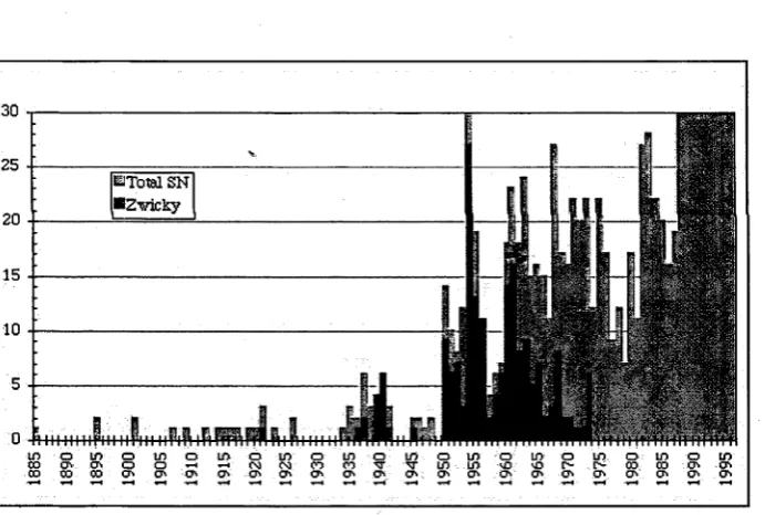
1.1 Supernovae discovered from 1885, when the first extragalactic event was found in M31, till the mid-nineties. The objects discovered by Zwicky and his collaborators (Gates, Humason, Johnson & Wild) are in red. Source: A. Bouquet, College de France & CNRS - Paris. 2

1.2 Spectra of recent Type-I supernovae, from the archive of the Harvard-Smithsonian Center for Astrophysics (Cambridge, Mass., USA). . . 4

1.3 Light curves of the various supernova types and subtypes (from Wheeler, 1990)... 7

1.4 An updated version of the Phillips relation between absolute mag nitude and decline rate (Ami5) for a sample of SNe la (left) and a subsample of these (right) which excludes higly reddened objects

(from Phillips et al., 1999)... 9

1.5 Supernova taxonomy (M. Montes, 2002, in http://rsd-www.nrl.navy.mil/7212/mon

) ... 10

1.6 Light curve of a normal SN la (SN 1992A) and of a few peculiar ones (From http:/ / garage.physics.iastate.edu/ astro505/ firstwk.html). 11

1.7 Left: The range of lightcurves for low-redshift supernovae of known relative brightnesses discovered by the Calän/Tololo Supernova Sur vey. Right: The same lightcurves after calibrating the supernova brightness using the stretch of the timescale of the lightcurve as an indicator of brightness (and the color at peak as an indicator of dust absorption). From Perlmutter et al. (1997)... 12

(11)

xii

1.9 Schematics of the explosion of a white dwarf near the Chandrasekhar mass. A thermonuclear runaway occurs near the center and a burn ing front propagates outwrards. Initially, the burning front must start as a deflagration to allow a pre-expansion because, other wise, the entire WD would be burned to Ni. Alternatively, the pre-expansion may be achieved during the non-explosive burning phase just prior to the thermonuclear runaway. Subsequent burn ing is either a fast deflagration or a detonation. In pure deflagra tion models, a significant amount of m atter remains unburned at the outer layers, and the inner layers show a mixture of burned and unburned material. In contrast, the models making a transition to a detonation produce the observed layered chemical structure with little unburned matter, wiping out the history of deflagration. Note that all scenarios have a similar, pre-expanded WD as an interme diate state... 16 1.10 Left:Snapshot of the front geometry of a 2D supernova simulation.

The center of the star is at the bottom left corner of the diagram. Right: Front geometry in a 3D run. Only one octant of the star has been simulated. The center is located at the back lower left corner. From: M. Reinecke, W. Hillebrandt and the Hydrodynamics Group at MPA, Garching (Germany)... 18 1.11 Distribution in the sky (RA on the x-axis, Dec on the y-axis) of all

SN discovered from 1885 till the mid-nineties described in Figure 1.1. Source: as in Figure 1.1... 20 1.12 Right: NGC 1365 with SN 2001du in an APT image taken in August

2001 (see IAUC N. 7690). Left: the SN, below the nucleus of the galaxy, is revealed by subtracting a template of the same field from the image on the right... 22

2.1 Figure: Location of the telescopes used for the photometric (green dots), spectroscopic (black dots) and infrared (red dots) follow up of SN 2003kf... 30 2.2 The FLWO 1.2m telescope at Mt.Hopkins, Arizona, used by

Math-eson et al. at CfA to follow SN 2003kf in the UBVRI photometric bands... 32 2.3 Flat field in the U band taken at the 2.3m telescope + Imager on

(12)

xiii

2.4 Point Spread Function (PSF) of SN 2003kf observed in R band at the Nordic Optical Telescope on December 14, 2003. Since the supernova was still very bright at that phase, the uneven galaxy background is not obvious in this image... 39 2.5 A V-band image of SN 2003kf taken at the TNG on December 17,

2003 (right) and the same image after performing PSF-subtraction on the supernova and a number of field stars (left). A residual is present around the PSF-subtracted brighter stars, which is mini mum around the stars of average magnitude in the image (as the SN should be)... 40 2.6 Local star sequence of SN 2003kf in a V-band image taken at the

NOT on December 14, 2003... 42 2.7 The result of our empirical correction of the B filter of the 2.2m tele

scope at Calar Alto to match the standard stars color term (dotted line) with the original Ca2.2m B filter passband (left) and the stan dard Johnson’s system B passband (right)... 45 2.8 Plots of AB-B ( y axis) versus B-V of the synthesized magnitudes of

the local sequence standard stars, with the exclusion of the reddest ones, for the above filter un-tweaked (left) and tweaked (right). . . . 45 2.9 Early light curve of SN 2003kf in the V band: a comparison between

the data from the RTN telescopes and the data from the FLWO 1.2m telescope...46 2.10 UBVRI light curves of SN 2003kf at early phases. Except for the

V magnitudes, the others have been shifted by the values shown in the figure...47 2.11 Relation between Am15(B) and absolute magnitude in B (left panel)

and V (right panel) for a sample of SNe la. The solid line is the fit measured for each relation by Hamuy et al. (1996)... 48 2.12 Complete V and R light curves. The R magnitudes have been

shifted as indicated... 49 2.13 Reddening-corrected B-V colour curves of a sample of SNe la (see

Chapter 3, Table 1) for description of data... 50 2.14 Undereddened B-V (left) and V-R (right) colour curves of SN 2003kf

superimposed to the relevant templates in Nobili et al. (2003) and their reddened (dotted line) and reddened+shifted version (dashed line)... 51 2.15 Undereddened V-I (left) and R-I (right) colour curves of SN 2003kf

superimposed to the relevant templates in Nobili et al. (2003) and their reddened (dotted line) and reddened+shifted version (dashed line)... 51 2.16 Early B light curve of SN 2003kf fitted by the Leibundgut B tem

(13)

x iv

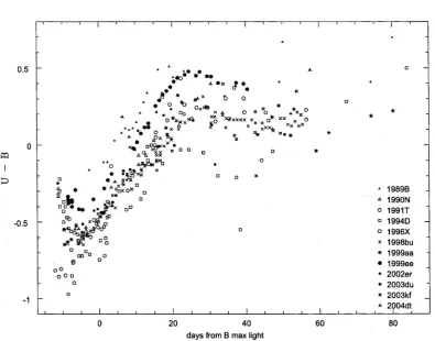
2.17 Reddening-corrected U-B colour curves of a sample of SNe la (see Chapter 3, Table 1 for description of data)... 53 2.18 U-B colour curve fit of the 10 SN la templates shown in Figure 2.17

with standard deviation curves, superimposed to the data points. . 53 2.19 Spectrum taken at the Calar Alto 2.2m telescope + CAFOS (Blue

Arm) on December 22, 2003. The supernova spectrum is the vertical black trace in the centre, the host galaxy is visible as a faint shade on the righthand side of the spectrum, the horizontal lines are due to the sky background. The black dots throughout the image are cosmic rays, and the two faint traces on the right are spectra of objects at the edge of the slit at the time of exposure... 61 2.20 The complete spectral sequence of SN 2003kf. The spectra have

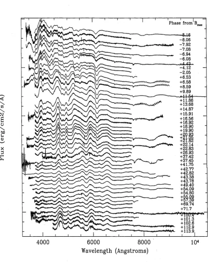
been arbitrarily scaled and shifted along the vertical axis, but not dereddened and not deredshifted...63 2.21 Ca II IR triplet profiles of SN 2003kf and other SNe la at early

phases (courtesy V.Stanishev)... 64 2.22 Expansion velocities for the Sill 6355Ä line for SN 2003kf compared

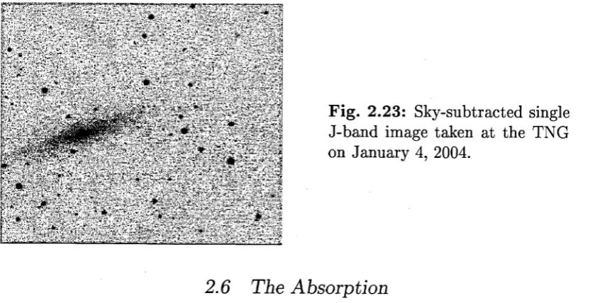
with those of SN 1996X (red triangles)... 67 2.23 Sky-subtracted single J-band image taken at the TNG on January

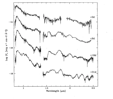
4, 2004... 68 2.24 Infrared spectral sequence in the bands I to K taken at the UKIRT.

All the spectra but the one at +9d have been shifted by an arbitrary quantity for better display... 69 2.25 Wavelength-calibrated spectrum taken at the 2.3m telescope on

November 30, 2003, showing Ca lines at the redshift of our galaxy (A and C) and at the redshift of the host galaxy (B and D) of SN 2003kf... 70 2.26 Spectrum taken at the NOT on December 13, 2003, showing Na

lines at the redshift of our galaxy (A) and at the redshift of the host galaxy (B)... 71 2.27 The colour curve fit for Type la supernovae in Phillips et al (1999,

solid line) overplotted on the colour curve of SN 2003kf. The line has been moved upwTard by adding the value 0.23 to the values of B-V calculated by Phillips et al... 71 2.28 Extinction curve of Savage & Mathis (1979) plotted against the

colour excesses in V,R,I,J,K... 72 2.29 Figure 1 of Benetti et al. (2005) showing the time evolution of the

(14)

X V

2.30 High velocity Ca II IR triplet (the broad absorption feature on the left) in the 2.3m spectrum of SN 2003kf taken on November 29, 2003. 76 2.31 Distribution of Ami5(B) for a sample of normal SNe la (solid line),

for 1991bg-like (dashed lines on the right of solid line. Dashed line at Ami5(B)=1.7 corresponds to SN 1986G), and 1991T-like (dashed lines within the solid line). Data from Reindl et al. (2005) and references therein... 79

2.32 Distribution of (B-V)o?max colors for a sample of normal SNe la (solid line), for 1991T-like (dashed lines within solid line) and 1991bg- like (other dashed lines). Data from Reindl et ab, 2005, Table 2. . . 79 2.33 Distribution of Equivalent Width of the Sill 6355 Ä line for normal

SNe la around maximum (solid line) and for SN 1991T, SN 1997br, SN 1999aa, SN 2000cx and SN 2002cx (dashed line). The dashed line at EW=70 is the unusual SN 1999aa, the solid line at EW=190 is SN 2004dt... 80 2.34 EW of the ie-shaped SII feature between 5200 and 5700 Ä vs.

Am15(B) for a sample of SNe la ... 80 2.35 EW of the to-shaped SII feature between 5200 and 5700 Ä vs. the

ratio of the right and left components of the feature for the same sample of SNe la ... 81 3.1 The Figure 1 from Benetti et al. (2005) shows three different sub

groups of SNe la, related to the photospheric expansion velocity of the Sill element, which they identified through Hierarchical Cluster ing Analysis. SNe 1991bg, 1997cn and 1999by are faint SNe la, the ones on the upper right until SN 199IT are normal SNe la with low velocity gradient and the others are normals with a high velocity gradient... 86 3.2 Mazzali et al. (1998) find a relation between the line width of

4700Ä Fe in nebular SNe la spectra at and their Ami5(B) decline rate parameter... 88 3.3 Complete early B light curve of SN 1994D (x-axis: days from B

max.light, y-axis: magnitude) fitted with a 4th order polynomial. . 91 3.4 Mean spectrum (upper left), first Principal Component (upper right),

second Component (lower left) and summary plot (lower right) of SN la spectra around maximum light... 99 3.5 Mean spectrum at maximum light (bottom), with the first compo

(15)

xvi

3.6 Mean spectrum, first and second components of spectra between -15 and -9 days from maximum light...101 3.7 Weights for the first and second components for spectra between

-15 and -9 days... 102 3.8 Bottom: mean spectrum at phase -12 days; middle: first com

ponents of SNe 1999ac (solid line) and 1994D (dotted line) have been added to the mean spectrum; top: second components of SNe 1999ac i solid line) and 1994D (dotted line) have been added to the middle spectra... 102 3.9 Mean spectrum, first and second components of spectra between -8

and -4 days from maximum light... 103 3.10 Weights for the first and second components for spectra between -8

and -4 days... 104 3.11 Bottom: mean spectrum at phase -6 days; middle: first components

of SNe 2002bo (solid line) and 1990N (dotted line) have been added to the mean spectrum; top: second components of SNe 1994D (solid line) and 2004dt (dotted line) have been added to the mean spectrum. 104 3.12 Mean spectrum, first and second components of spectra between -3

and 1 days from maximum light... 105 3.13 Weights for the first and second components for spectra between -3

and 1 days... 106 3.14 Bottom: mean spectrum at phase -1 days; middle: first components

of SNe 1996X (solid line) and 1999ac (dotted line) have been added to the mean spectrum; top: second components of the same SNe

(solid and dotted line respectively) have been added to the mean spectrum... 106 3.15 Mean spectrum, first and second components of spectra between 2

and 6 days from maximum light... 107 3.16 Weights for the first and second components for spectra between 2

and 6 days... 108 3.17 Bottom: mean spectrum at phase 4 days; middle: first components

of SNe 2002er (solid line) and 1998aq (dotted line) have been added to the mean spectrum; top: second components of SNe 2004dt (solid line) and 1992A (dotted line) have been added to the mean spectrum. 108 3.18 Mean spectrum, first and second components of spectra between 7

and 13 days...110 3.20 Bottom: mean spectrum at phase 10 days; middle: first components

(16)

x v ii

3.21 Mean spectrum, first and second components of spectra between 17 and 23 days from maximum light... I l l 3.22 Weights for the first and second components for spectra between 17

and 23 days... I l l 3.23 Bottom: mean spectrum at phase 20 days; middle: first components

of SNe 1991T (solid line) and 2004eo (dotted line) have been added to the mean spectrum; top: second components of the same SNe (in the same order) have been added to the mean spectrum... 112 3.24 Mean spectrum, first and second components of spectra between 25

of SNe 2002er (solid line) and 1999ac (dotted line) have been added to the mean spectrum; top: second components of the same SNe (in the same order) have been added to the mean spectrum... 114 3.27 Mean spectrum, first and second components of spectra between 50

and 70 days from maximum light...115 3.28 Weights for the first and second components for spectra between 50

of SNe 1981B (solid line) and 1996X (dotted line) have been added to the mean spectrum; top: second components of SN 1990N (solid line) and SN 1999aa (dotted line) have been added to the mean spectrum...116 3.30 Mean spectrum, first and second components of spectra between

100 and 300 days...116 3.31 Weights for the first and second components for spectra between

100 and 300 days...117 3.32 Bottom: mean spectrum at phase 200 days; middle: first compo

nents of SNe 1981B (solid line) and 2004eo (dotted line) have been added to the mean spectrum; top: second components of SN 1994D (solid line) and SN 2002er (dotted line) have been added to the mean spectrum...117 3.33 Supernovae at around 6 days before maximum light. The spectra

(17)

xviii

4.1 P-Cygni profiles are typical of spectral lines caused by fast expand ing shells. They show a blueshifted absorption coupled with a broad emission at rest wavelength. (From an online tutorial by D. Kasen, http://supernova.lbl.g o v /^ d n k a s e n /tu to ria l/)... 125 4.2 Supernova spectra at early phases (D. Kasen, URL as in Figure 4.1). 127 4.3 Spectrum of SN 2003ch observed at the 2.3m telescope and classified

with SNID...129 4.4 SNID output table showing the results of cross-correlation between

a spectrum of SN 1996X and a number of SN la templates... 130 4.5 Phase distribution of the 538 spectra in our sample. The phase is

expressed in days past B maximum light... 131 4.6 SN 1981B at 17 days past maximum light, matched by SN 2003kf

at 20 days past maximum...132 4.7 SN 1986G at 2.61 days before maximum light, matched by SN

2004eo at 6.6 days before maximum light... 133 4.8 SN 1990N 227 days after maximum light, matched by SN 2003du

at 222 days past maximum light... 134 4.9 SN 1991T 67 days after maximum light, matched by SN 1999aa at

51 days past maximum... 135 4.10 SN 1991bg at maximum light, matched by SN 1986G at the same

phase...136 4.11 SN 1991bg at 54 days past maximum light, matched by SN 2004eo

at 73 days...136 4.12 SN 1992A at 2.6 days past maximum matched by SN 2003kf at 6.5

days past maximum...137 4.13 SN 1994D at 10 days before maximum light matched by SN 2002bo

at the same phase... 138 4.14 SN 1996X at maximum light matched by SN 1994ae at phase 2 days. 139 4.15 SN 1997br at 17.4 days past maximum matched by SN 1999ee at

16.5 days... 139 4.16 SN 1999aa 7 days before maximum light matched by SN 2000cx at

-3 days... 141 4.17 1999ee 2 days after maximum light matched by SN 1 9 9 9 a c ... 142 4.18 2000cx 2 days after maximum light matched by SN 1999ee 1.5 days

before maximum...142 4.19 SN 2002bo at 2.6 days before maximum light matched by SN 2002er

at 1.5 days before maximum... 143 4.20 2002cx at 16d past maximum matched by SN 1997br at 23 days

past maximum...144 4.21 Flux calibrated spectrum of SN 2002er 8 days before maximum

(18)

x ix

4.22 2004dt one day before maximum light matched by SN 1994D at the same phase... 146 4.23 2004eo 11 days before maximum light matched by SN 1999ac 2 days

past maximum... 147 4.24 (Continued from previous page) Histograms of the differences be

tween real phase and SNID phase within the phase bins indicated. The solid line is limited to the normal SNe la in our sample, the dashed line includes the peculiars as well... 151 4.25 The average errors in phase determination shown in the previous

figure are plotted here as a function of the phase bins. The solid line refers to normal SNe la, the dashed lines to all SNe la of our sample...151 4.26 The spectra of the template SN 1994D as they are recorded in the

file “sn94d.lnw” ...155 5.1 Benetti et al. (2004) show in this Figure that the relationship be

tween Rs u i ratio and decline rate (which is related to the absolute magnitude) seems to break down below a certain value...164 5.2 The position of the SNe la in our database with respect to the

(19)

(20)

x x i

LIST OF TABLES

2.1 Journal of photometric observations... 35

2.2 Detectors used for the monitoring of SN 2003kf and their charac teristics... 36

2.3 Constant terms b and color terms a calculated for the telescopes that observed standard stars with the same setup used to observe SN 2003kf... 41

2.4 True magnitudes of the local sequence stars around SN 2003kf. a is the RMS error on the measurements and N is the number of stars used to calculate the reported values... 43

2.5 Important photometric quantities for SN 2003kf in the optical pass- bands: magnitude at maximum light, Julian Date of maximum light (minus 2450000.00), and decline rate at early and late phases. . . . 49

2.6 Polynomial fit to our U-B data points as it appears in Figure 2.18 with standard deviation. The phase is expressed in days past B maximum light... 54

2.7 Photometry of SN 2003kf. Error in the measurements and k-correction applied are also listed... 57

2.8 Journal of Spectroscopic Observations... 60

2.9 Photospheric velocity of the Sill 6355Ä line... 66

2.10 IR coverage of SN 2003kf... 66

2.11 IR magnitudes of SN 2 0 0 3 k f... 67

2.12 Unreddened observed magnitudes, absorption and absolute magni tudes of SN 2003kf... 74

2.13 A set of properties within which a SN la can be considered normal. 77 3.1 Main quantities of all the supernovae used for our study... 97 4.1 Spectra contained in the new SNID template library. The phase is

(21)

(22)

“Between two worlds life hovers like a star, ’Twixt night and morn, upon the horizon’s verge, How little do we know that which we are,

How less what we may be!”

(23)

(24)

1. INTRODUCTION

1.1 The origins o f supernova research, with particular reference to

their use as distance estimators

In the 1920’s scientists begun to realise that there was a particular class of very bright novae (Lundmark, 1920, Curtis, 1921). A decade later, Baade and Zwicky at the California Institute of Technology defined them supernovae (SNe hereafter; Zwicky, 1938). The new word was not immediately accepted by the scientific com munity. For example, supernovae are not mentioned in Hubble’s The Realm of the Nebulae, 1936 (according to Zwicky, 1961). The distinction between novae and

supernovae was at first based on twelve objects discovered between 1895 and 1930, plus the galactic SN observed by Tycho in 1572. SN events in our own Galaxy are often heavily dimmed by the interstellar dust, and only a few of them have been recorded in the past millennia. Among them, the supernova observed in 1604 by Kepler, others observed in 1181, 1054 (which produced the Crab Nebula), 1006, and a few earlier and less certain ones. All the Galactic supernovae have been ob served with naked eye, as unfortunately the last event observed in the Milky Way occuTTed five years before Galileo pointed the first telescope at the sky, therefore those data are difficult to compare with modern observations of extragalactic SNe. In the same year when Hubble’s book was published, the first systematic super nova search was started by Baade and Zwicky using the Palomar 18-inch Schmidt telescope and led to the discovery of 19 SNe between 1936 and 1941.

Two supernovae discovered in 1937, 1937C1 and 1937D, provided the first well sampled light curves and spectra. Minkowski remarked the strong similarity be tween these two objects in their spectroscopic and photometric evolution and, as it happened that both these objects and the other few ones discovered at that epoch were SNe I, he deduced that SNe in general have very similar characteristics. SN 1937C, observed for about two years, was for decades the template SN I. Baade (1938) found an average absolute magnitude of the few SNe discovered to date M0 = -14.3, with a dispersion a = 1.1. This very small dispersion value led Zwicky and Wilson to suggest the use of SN as distance indicators (Trimble, 1982). In

(25)

2 I n tr o d u c tio n

the following years, however, a few SNe of a different kind were discovered, and Minkowski (1941) proposed the division of the class in Type I (SNe I) and Type II (SNe II), distinguished by the presence or lack of Hydrogen lines in their early spectra. SNe I seemed to be a homogeneous group, brighter on average than SNe II, and therefore still a suitable distance estimator, while the observations showed immediately that SNe II can be quite different from each other in their light curves and magnitudes at maximum.

In the Fifties, although there were no systematic searches, the number of SN discovered grew to 54, but the best-studied objects remained the two discovered in 1937. Borst (1950) noted that the most likely source to power SNe I during their decline, observed in SN 1937C with a gradient of 0,137 mag/day at 100<t<635 days past maximum light, wras the decay of a radioactive nucleus. Baade et al (1956) suggested 2o4Californium to be responsible for the light curve decline, as its half-life of 55±1 days provides a rate similar to the observed, but they were not able to test their theory against observations as no satisfactory identification of SN spectral lines was available at the time.

25

---«Total SN ■ Z v ic k y

■ I f f 1 H t H--H H H -W H H 4 i T > o i r > O L O o i n o m o L O o m o L n o L O O i r > O L n o i r > oo cr. cr. o o —« —< oo co co oo 'T l d uo ■jd ■jd r- r- öd >:o a- as

0Q CO CO CT- Qs CT> Qs O ' QS O ' Qs Qs c F O ' q s q\ q\ q s q\ q s ct> Qs Qs

tH*H »H tH tH tH*H rH rH rH *H tH vH«-H »H vH*H ( tH

Fig. 1.1: Supernovae discovered from 1885, when the first extragalactic event was

found in M31, till the mid-nineties. The objects discovered by Zwicky and his collaborators (Gates, Humason, Johnson & Wild) are in red. Source: A. Bouquet, College de France &; CNRS - Paris.

[image:25.527.39.385.327.560.2]

(26)

1.2 N e w m o d e ls an d n e w d a ta se ts 3

attempts to obtain the average absolute magnitude for supernovae were made by Minkowski (1964). However, as only few of the 122 SNe discovered so far had published data, Minkowski’s work still heavily relied on Baade’s measurements. By the end of the Sixties the set of observational data has exploded considerably, with light curves available in photographic, V and B bands for a few tens of objects (see Figure 1.1).

1.2 New models and new datasets

Kowal (1968) included nearly 40 light curves in his extensive work on photomet ric data, which provided a reliable photographic magnitude for SNe at maximum. He found MP5 = -18.6+51og(H0/100) for Type I, M pg = -16.5+51og(H0/100) for Type II, both with <r=0.6. Kowal recognized the usefulness of SNe I as distance indicators, predicting that their magnitude could be determined with an accuracy of 0.1, 0.2 mag in clusters of galaxies. However, he pointed out that SNe alone cannot be used to measure the Hubble constant because still unreliable determi nation of their distance moduli prevented a proper calibration of SNe I from being obtained. The change in this would come when distances of the parent galaxies would become available using different methods such as Cepheids, HII regions or red supergiants.

Colgate & McKee’s (1969) models increased dramatically our understanding about supernova explosions from a theoretical point of view, and this was one of the reasons th at prompted observers to put a good deal of effort in taking SN spec tra. Till then, the only well studied SN was 1937C, with a long series of spectra by Minkowski. The new models predict the light curve absolute maximum and decline based on the amount of o6Ni produced in the explosion. The energy is supplied by the decay of o6Ni to o6Co (6 days) near maximum light and of o6Co to 56Fe (77 days) together with progressive 7-ray transparency of the ejecta during the long-time exponential light decay.

(27)

4 In tr o d u c tio n

the various phases. Their work ruled out the earlier viewT suggested by Minkowski (1939, 1941) that the SN spectra consist of emission bands of highly ionized and excited gas, while it confirmed what found by Patchett & Branch (1972): the presence of absorption lines in SN spectra suggests the possibility of accounting for the light curves in terms of thermal emission from an expanding, optically thick photosphere. As regard to SNe I, the spectra are a superposition of P-Cygni profiles upon a continuum. Some examples of SN I spectra can be seen in Figure 1.2.

SN 2004aw 2004-03-21

SN 2003jd

SN 2001V day-1 4

5000 6000

Res’. Wav «.length (A)

Fig. 1.2: Spectra of recent Type-I supernovae, from the archive of the Harvard- Smithsonian Center for Astrophysics (Cambridge, Mass., USA).

[image:27.527.56.351.189.443.2]

(28)

1.2 N e w m o d e ls and n ew d a ta se ts 5

As a different approach to use SNe I as distance indicators, Barbon, Ciatti and Rosino (1973, hereafter BCR) constructed an average light curve using all the SN I light curves available in the literature and those taken at Asiago Observatory, and calibrated it with Kowal’s zero point. BCR found that there are ’’fast” and ’’slow” SNe I, the former brighter by ~0.32 mag. On a similar strategy, Pskovskii (1969) parameterized the light curve shape instead of dividing the objects in two subclasses and found a relation between decline rate (expressed in mag/1 OOd) and absolute magnitude, but of different sign than BCR’s. Due to this difference in trend, the astronomical community looked at the results found by Pskovskii and BCR with skepticism for more than a decade, on the ground that the errors due to photometry, galaxy absorption and other factors do not allow any such trend to be detected, and that the host galaxy contamination would produce a similar effect to the trend found by Pskovskii (Boisseau and Wheeler, 1991). Barbon et al. (1979) examine SNe II in order to investigate their use as distance estimators. They find that SNe II can be divided in two subclasses, II-P and II-L, based on their light curve shape, and that SN II-P are a quite homogeneous group. They find the average absolute magnitude of SNe II and a dispersion of 0.78.

Branch (1981), measuring the wavelength of the 6130Ä absorption feature in the spectra of 16 SNe I, finds that the “fast” and “slow” SNe I as defined by BCR based on their light curve shape have significantly different expansion velocities. He also confirms the result by Pskovskii (1977) that expansion velocity and ab solute peak magnitude are correlated wdth the light curve decline rate. Branch and others w-arn that SNe I might have a total range of ~2 mag in absolute B magnitude (Trimble, 1982 and references therein). On the other hand, Sandage and Tammann (ST, 1982) do not believe in any such correlation, as they claim it would be hidden within the photometric errors. They find the distance moduli of the host galaxies of SN 1937C and SN 1954A using the brightest red supergiants and, after showing that o m b of SNe I at maximum light is small (a few tenths

at most), they use the mean absolute magnitude of these two SNe to calibrate the Hubble diagram for 16 SNe I. In the same period, SN 1981B is discovered that becomes the third most important template after SNe 1937C and 1972E. It is found photometrically very similar to the latter, thus supporting the thesis by ST rather than the suggestion by Pskovskii and BCR of a relation between absolute magnitude and decline rate.

(29)

6 In tr o d u c tio n

In the process, Arnett finds that the trend described by BCR is reproduced by his method.

In 1984 a favourite model to describe SN I explosions, the W7 model, is pre sented (Nomoto, Thielemann and Yokoi), a carbon deflagration in an accreting C -0 White Dwarfs. The radioactive decay of the 0.5-0.6 M0 of o6Ni synthesized, and the following decay of o6Co and o6Fe, power the light curve. Intermediate mass elements such as Ca, Ar, Si. S, Mg and O are synthesized in the decaying deflagration wave, which is consistent with SN I spectra near maximum light. But the issue remains open whether SNe I are a homogeneous class as suggested by Tammann and his collaborators or if they are not as suggested by Pskovskii and BCR.

1.3 SN I subclasses

In 1985 a pattern emerges. Uomoto and Kirshner (1985) note that SN 1983N seems to be 1.4 mag fainter that the average SNe I, and that the 6115Ä feature normally present in SN I maximum-light spectra is missing in its spectra. They also note that two other SNe I showed the same peculiarity and suggest that these three events are different from both SNe I and SNe II. These events are easily recognizable from their color curves after maximum light. A similarity between SN 1983N and other peculiar SNe I is noted also by Sramek et al. (1984). It is not the first time that some authors recognized peculiar objects among SNe I: Bertola (1964) had already noted that there are SNe I without the main 6115Ä feature; Oke & Searle (1974) had found three significantly peculiar SNe I: 1954A, 1962L, and 1964L. The novelty is that researchers in the Eighties notice some systematics in the peculiarity. Wheeler & Levreault (1985) note that a spectrum of SN 1984L is very similar to that of SN 1983N and infer that these two objects belong to a very homogeneous and underluminous class of peculiar SNe I (SNe Ipec). Such SNe Ipec would have less Nickel mass than normal SNe I and would derive from core collapse, like SNe II, rather than from thermonuclear burning, like the other SNe I.

Uomoto & Kirshner, as well as Wheeler & Levreault, recommend to remove SNe Ipec from any sample of SNe I when using it to estimate distances. Their claim of the existence of a subclass of SNe I with SN 1983N as a template is supported by the fact that this object, and SN 1984L, are the first SNe I to be detected in the radio (Sramek et al., 1985). Before then, only SNe II had been detected in the radio, although observations of SNe I had been made at those wavelengths.

(30)

B

L

U

E

MA

GNIT

UDE

1.4 C a lib r a tin g S N e as d ista n c e e s tim a to r s 7

SN I9 8 7 A

150 2 0 0 3 0 0 3 5 0 DAYS AFTER MAXIMUM LIGHT

Fig. 1.3: Light curves of the various supernova types and subtypes (from Wheeler,

1990).

identifiable in the IR colour curve, as SNe lb do not show the variable absorption at 1.2 micron which is typical of SNe la. Branch (1986) notes that SNe la are the vast majority of SNe I, and that a few SNe Ipec exist which do not correspond to the 1983N-like SN lb subclass defined by Elias et al.. Moreover, it is still evident th at SNe la exhibit a rather wide scatter in absolute magnitude, and Branch explores this issue during the following years. In 1987 he shows that the expansion velocities in SN 1984A spectra are significantly larger than those shown by the ” normal’’ SN 1981B (see also Branch et al., 1988). But the most ”different” SNe la found in the Eighties is undoubtedly SN 1986G. Although heavily dimmed, it shows clear photometric and spectroscopic (narrower lines) peculiarities respect to the other SNe la. Figure 1.3 shows the average B light curves of the various SN types and subtypes and their relative brightness.

1.4 Calibrating SNe as distance estimators

(31)

8 In tr o d u ctio n

Leibundgut (1988) presents multicolour light curve templates for SNe la and finds that the differences between the single objects and the templates are within the photometric errors. The great uniformity of light curves and spectra can be explained with the decay of Ni and Co in a Chandrasekhar ejected mass.

Early in the Nineties, CCD observations of SNe become available and allow a better investigation of light curves and spectra. A new subclass of SNe I, SNe Ic, is spectrosopically isolated by Harkness Sz Wheeler (1990). New well observed SNe la, SNe 1989B and 1990N, are available as templates. Leibundgut et al. (1990) show th at at least for some SNe la the use of template light and color curves is justified, the exception being, among the recent SNe la, SN 1986G. Leibundgut & Tammann (1990) find a mean absolute magnitude Mß=-19.79±0.12 for six su pernovae in the Virgo cluster, in gcod agreement with other determinations of the Virgo cluster distance. Apart from being useful as distance indicators, SNe la can help to measure the deceleration parameter (Leibundgut et al., 1990) and peculiar motions in the local universe (Miller & Branch, 1992). Miller & Branch (1990) find that SNe la in inclined spirals can be rather faint and infer that this is due to the reddening. They do not find confirmation to Pskovskii’s relation between absolute magnitude and decline rate, and they comment that this relation might be due either to systematic errors on photometry or to mere chance.

In 1991, SNe 1991T and 1991bg are discovered and they soon show obvious differences from every other SNe la. The optical spectra of SN 1991T before max imum were very different from those of the common SNe la, and its light curve decline was significantly slower than the template light curve (see e.g. Ruiz La- puente et al., 1992). SN 1991bg vas intrinsically redder than the templates (see e.g. Filippenko et al., 1992). They also appeared to be overluminous and underlu-minous respectively, thus disrupting the belief that most SNe la are very similar in their observed behavior and absolute magnitude. However, those who wanted to use SNe la as distance indicators vere not overly worried because the peculiarities of these SNe can be easily detected, hence such objects can be weeded out of the ” normal” SNe la (Branch & Tamnann 1992, Branch & Miller 1993).

(32)

1.5 Type la supernovae, the state of the art 9

-2 0

-1 9

- 1 8

- 1 7

I - 1 9 O)

§ - 18

I

ro " 17 E

^ -20

- 1 9

- 1 8

- 1 7

Fig. 1.4: An updated version of the Phillips relation between absolute magnitude

and decline rate (Ami5) for a sample of SNe la (left) and a subsample of these (right) which excludes higly reddened objects (from Phillips et al., 1999).

■ i

: - :

B :

T . .

B

: j

V t

: ; ' i— 4 — 1 :

V

. T ^ ’~ t H .

1

: ^ . . . 1 ' :

I

1.0 1.5 2.0 1.0 1.5 2.0

AnUBL*

because the variation in magnitude between the various SNe la at maximum light is smaller in the other bands, as shown in Figure 1.4. The Phillips relation was not accepted at once by the astronomical community due to the low number of objects used (nine) and the high number of peculiar ones in the sample, which does not match the actual rate between normal and peculiar SNe la.

1.5 Type

l a

supernovae, the state o f the art

(33)

10 In tr o d u ctio n

Spectra: No HydroSen / Hydrogen

SN I _{S N n}

Fig. 1.5: Supernova taxonomy (M. Montes,

www.nrl.navy.mil/7212/montes/snetax.html ).

2002, in

http://rsd-be produced by collapse of the core of massive stars. Therefore nowadays we prefer to divide supernovae in two other categories: Core-Collapse and Thermonuclear. The former show great observational diversity, which is supposedly due to the large variety in size of the progenitor and to environmental conditions. Some of the most powerful among these events seem to be related to Gamma-ray Bursts, they are called Hypernovae (Nomoto et al., 2005). The latter include only SNe la, which will be the topic of our discussion from now on.

1.5.1 SNe la and their use as distance estimators

(34)

1.5 Type la supernovae, the state of the art 11

indicator. This happened for SNe I when it appeared evident that another class, SNe II, existed and, since the Eighties, for SNe la.

The B light curves of SNe la show a rather steep rise to maximum light, which is reached two or three weeks after the explosion. After maximum, the SN dims by 0.1 mag per day until the so-called inflection point, reached usually at a phase of 25-30 days, when the decline rate becomes ~1.2 mag/100d. The V light curves show a similar behavior, with the maximum light generally occurring between 0.5 and 2 days after B maximum light. At times, the V light curves show a shoulder, corresponding to a plateau always visible in the R light curve, which becomes a secondary maximum in the I light curve. This I secondary maximum is not visible in some peculiar objects such as SN 1991bg. Examples of SN la light curves are visible in Figure 1.6.

1991bg 1992bo 1992A 1991T I992bc

20 40 60 80 - 2 0 0 20

Days Since B Maximum

Fig. 1.6: Light curve of a normal SN la (SN 1992A) and of a few peculiar ones

(From http:/ / garage.physics.iastate.edu/ astro505/ firstwk.html).

The slope of the B-V color curve of SN la is constant between 32 and 92 days from maximum light. Lira (1995) shows that the the evolution at these phases is remarkably uniform for SNe la in general. This can be used to calibrate the intrinsic colors of these objects at maximum light and to estimate the reddening

(35)

Fig. 1.7: Left: The range of lightcurves for low-redshift supernovae of known

relative brightnesses discovered by the Calan/Tololo Supernova Survey. Right: The same lightcurves after calibrating the supernova brightness using the stretch

of the timescale of the lightcurve as an indicator of brightness (and the color at peak as an indicator of dust absorption). From Perlmutter et al. (1997).

The magnitude-decline relation pointed out by Phillips was confirmed by Hamuy et al. (1995) using the SNe la discovered during the Calän-Tololo survey and the most populated sample we have to date is included in Germany et al., (2004). A similar way of comparing the relation between light curve shape and absolute magnitude of SN la, the stretch factor, is described in Perlmutter et al. (1997). By broadening or narrowing a SN light curve respect to the standard shape the lumi nosity of the object can be predicted and the light curve can then be normalised to the standard luminosity. See Figure 1.7 for an example of the effectiveness of this technique, which has later been improved with the Multi-Color Light Curve Shape method by Riess, Press &; Kirshner (1996). CMAGIC (Color-Magnitude Intercept Calibration, Wang et al., 2003) is a method to find the luminosity of a SN la observed after maximum light. It is based on the fact that the colour index in SNe la remains uniform for about a month after maximum. There is a color- magnitude relation which, after correcting for the decline rate, has a dispersion of 0.10 magnitudes.

(36)

1.5 T y p e l a su p e r n o v a e , th e s ta te o f t h e art 13

km/s at maximum light, and its velocity decreases at a slower rate than the rest of the photosphere in the following days. The continuum at this stage is similar to that of a B star. A week or so after maximum light, Ni-Co-Fe lines from the core start to appear, as the photosphere is retreating towards the inner regions of the expanding envelope. Eventually, at around three weeks after maximum light Fe lines dominate the entire spectrum, with some leftover Si or, a couple of months after max light, Co, Cr II and Na I. Spectra of SNe la at various phases are shown in Figure 1.8.

The homogeneity of SN la spectra at the various phases is such that one can determine the phase of a SN la by simply comparing its spectrum with a sequence of comparison spectra of similar objects. Nonetheless, the study of good quality data demonstrates that spectroscopic differences do exist between SNe la in gen eral, and not only between extreme cases such as, for example, SNe 1991T and 1991bg. Some of these differences define trends that might be useful in defining relations between absolute magnitude and spectral characteristics of SNe la.

One remarkable difference is that the continuum is bluer in SNe with lower values of Arai5 (B), which seems to be related to variations in temperature. The relation between the B absolute magnitude and the ratio of the Si II absorp tion lines at 5800Ä and 6150Ä described by Nugent et al.(1995) might also be temperature-related. Benetti et al.(2004) suggest that this relation breaks down at low values of Arais(B). Nugent et al.(1995) also find a relation between the ratio of the H and K Ca II absorptions and the B absolute magnitude, while Mazzali et al.(1998) find a relation between the FWHM of the 4700Ä Fe line in very late spectra and the Arais(B).

All these relations between photometric and spectroscopic characteristics of SNe la and their absolute magnitude have supported the hypothesis that one parameter is sufficient to describe the differences between the various objects. This was, therefore, the general belief among the supernova community at the end of the last decade. The new decade, and the new century, have brought with them a number of objects which defy this paradigm, and the tools to investigate the issue further.

1.5.2 Peculiar SNe la

(37)

M a x im u m (b )

A m u

J— v 94D 1.32 ^ + 0 .2 d

0 2 e r 1.3 3 / V - 0 . 3 d

1 0 0 0 0 - 1 w e ek (a )

9B aq -B d 0 2 b o - S . l d

0 2 e r - 7 4d : 6 0 0 0 0 0 0 0 1 0000

l w eek (c )

96X + 6 d J 0 2 e r + 5 .7 d 6 0 0 0 8 0 0 0

4 0 0 0 1 0 0 0 0

m

9 8 bu + 1 9 2d 9 8 a q +19(1

5 0 0 0 6 0 0 0

4 0 0 0 7 0 0 0 8 0 0 0

M*>

1 m o n t h (c )

0 2 b o 31 4d 96X 3 1 .3 d

0 2 e r + 3 3 6 d

4 0 0 0 5 0 0 0 8 0 0 0 7 0 0 0 0 0 0 0 9 0 0 0

MAI

Fig. 1.8: Spectra of a few SN la compared at representative phases (from Kotak

(38)

1.5 T y p e l a su p ern o v a e, th e s t a t e o f th e a rt 15

to be reproduced. We will discuss models in the next section but we will briefly examine here the general characteristics of a number of peculiar SNe la. We have seen how SN 1991T was the first peculiar SN la to be discovered, although SN 1986G (Phillips et al., 1987) had already cast some doubts on the uniformity of the class. The early-phase spectra of SN 1991T are nearly featureless and only after maximum light this object starts showing SN la characteristics. Its light curves are not peculiar, although its decline rate is slower than average and its luminosity seems to be higher than average. With the normal SN 1998bu (Cappellaro et ah, 2001), this is the only SN la to have produced a light echo. SN 1991bg, the second peculiar SN la discovered, has opposite characteristics: its light curves show a much faster decline than average and its spectra show Ti at bluer wavelengths, which is not visible in normal events. Its spectra remain peculiar also at late phases and its I-band light curve does not show the usual secondary maximum. These characteristics, and a much fainter magnitude than average, are the signature of a very low-energetic event. Like SN 1991T, SN 1991bg is now the representative of a well-populated class of objects. SN 2002ic (Deng et al., 2004) might also be considered the representative of a subclass formed by a few objects, although its very attribution to the class of SNe la is still controversial. Indeed, its spectra show a strong H line, which is the defining characteristics of Type II SNe, but this feature comes from a circumstellar shell, surrounding what looks like a normal SN la event. Other objects, such as SNe 1998Z, 1997cy, 1999E and 2005gj show similar characteristics. Some peculiar objects are the only representative of their class: this is the case for SNe 2000cx and 2002cx. The former wras the brightest SN discovered in the year 2000 and it was extensively observed by Li et al. (2001a). Its light curves show a different rate between rise and decline - a speedy rise to maximum light and then a slow decline - the colour curves show an unusual evolution and the spectra, initially similar to those of SN 1991T, are different from the average until after maximum light. SN 2002cx (Li et al., 2003) shows an opposite discrepancy in its light curve: a slow rise and a fast decline, together with a much fainter magnitude than any known SN la. Its spectra, apart from the early ones which are featureless like SN 1991T, remain different from average at all phases. The datasets of all the peculiar objects we have described, with the exception of SN 2001ic, are included in our work and will be described in more detail in the following chapters.

1.5.3 Progenitors o f SNe la

(39)

Initial WD DeJlagraiion pliase(2..,3see) Deionaiiou phase (0.2...0.3 sec) pro-expansion of Lhc WD hardly any time fo: father expansion

Fig. 1.9: Schematics of the explosion of a white dwarf near the Chandrasekhar

mass. A thermonuclear runaway occurs near the center and a burning front prop agates outwards. Initially, the burning front must start as a deflagration to allow a pre-expansion because, otherwise, the entire WD would be burned to Ni. Al ternatively, the pre-expansion may be achieved during the non-explosive burning phase just prior to the thermonuclear runaway. Subsequent burning is either a fast deflagration or a detonation. In pure deflagration models, a significant amount of m atter remains unburned at the outer layers, and the inner layers show a mixture of burned and unburned material. In contrast, the models making a transition to a detonation produce the observed layered chemical structure with little unburned matter, wiping out the history of deflagration. Note that all scenarios have a similar, pre-expanded WD as an intermediate state.

with the ejecta of a SN II (Starrfield, 2003). The nature of the companion star in these systems, however, has not been fully explained to date. We can only infer that it must be an evolved star, as we do not see any H or He in the ejecta of SNe la, so this kind of mass cannot be the material that the WD accretes. A simplified model of SN la explosion (from Höflich, Gerardy, Linder & Marion, 2003) is shown and described in Figure 1.9.

Mass of the progenitor: it is currently believed (Nomoto et al., 2003) that the WD accreting mass from the companion star explodes when it reaches the crit ical mass M~1.37-1.38M0 near the Chandrasekhar mass. At this point the star begins to contract, causing carbon ignition in the central region and a thermonu clear runway, and it is eventually completely destroyed. The synthetic spectra produced with this method are in excellent agreement with the observed ones, although there might be peculiar events whose behaviour is better described by sub-Chandrasekhar mass models. For example, SN 2000cx has a very blue spec trum at early phases, and synthetic spectra derived from sub-Chandrasekhar mass models are also very blue.

(40)

1.5 T y p e l a su p ern o v a e, th e s ta te o f th e art 17

which is consistent with a SN la event, but it seems more likely to produce a core collapse SN rather than a thermonuclear explosion. The SD scenario is therefore the most promising of the two as far as SNe la are concerned. Several types of binary systems have been proposed at different times as progenitors for SNe la. However, many of them (Classical Novae, Dwarf Novae, Symbiotic Variables and Symbiotic Novae) would produce too much H and He, that we do not see in the spectra. According to Baron et al (2001, private comm, to Starrfield) SN la can only produce 0.1M© or less of Hydrogen.

We will now consider the only two different binary systems that might generate a SN la according to the SD scenario. The first one is a WD+RG system (sym biotic system), it can be observed as symbiotic stars, luminous supersoft X-ray sources or recurrent novae. The second one is a WD+MS system, in which a C+O WD is formed from a red giant that transfers part of its outer envelope on the companion main-sequence (MS) star. Such systems are visible as supersoft X-ray sources and some recurrent novae, like U Sco. The rate of SNe la inferred from the estimated frequency of these systems is ~0.003/yr, fairly close to the inferred rate of SN la in the Milky Way.

M o d e ls

For the last thirty years, theorists have used one-dimensional, spherically symmet ric models to describe the observed behavior of SN la. High accretion rates cause a higher central temperature and pressure, favoring lower ignition densities. A flame front then propagates as a deflagration wave due to heat transport across the front. These models can reproduce the observed characteristics of SN la events by parameterizing the thermonuclear flame speed and, in case, the density at which a spontaneous transition to supersonic burning (detonation) occurs. Multidimen sional calculations of deflagrations, on the other hand, allow to determine the energy generation rate independently from the local value of the flame speed. In the past couple of years three-dimensional modelling of SN la has become possible (Niemeyer, 2003). 3-D hydrocodes well account for the deformation of the flame surface, which determines the acceleration of the fuel consumption rate, having the initial configuration of the flame as the main free prameter. The ability of these models to reproduce observations strongly depends on the resolution of the simulation (see Figure 1.10 for an example).

The current preliminary results show that the Chandrasekhar mass scenario with pure turbulent deflagration is a viable candidate for SN la explosions, but a

/