Parallel processor implementation in computerized tomography using transputers : a thesis presented in partial fulfilment of the requirement for the degree of Master of Technology in Production Technology at Massey University

PARALLEL PROCESSOR IMPLElVIENTATION

IN COMPUTERIZED TOMOGRAPHY USING

TRANSPUTERS

A THESIS PRESENTED IN PARTIAL FUFILMENT OF THE

REQUIREMENT FOR THE DEGREE OF MASTER OF TECHNOLOGY IN PRODUCTION TECHNOLOGY AT MASSEY UNIVERSITY

WENJUWU

Abstract

Acknowledgements

I wish to express my sincere appreciation to my supervisor, Dr. Bob Chaplin, for his guidance throughout this project.

I would like to thank Prof Bob Hodgson and Dr Bob Chaplin for their help and care during the course ofmy study, Dr Roger Browne for his help throughout the project and Mr White Page for his help in image research.

My thanks also extend to Dr Paul Austin, Dr Huub Bakker, Mr Ralph Pugmire, Dr Clive Marsh, Mr Merv Foot and all staff in the Production Technology Department of Massey University for their help and friendship.

I wish to gratefully acknowledge Mr Phil Long for all his help during my research period.

Table of Contents

Abstract .. ... ... .. .. .. . . ... .. . . .. . .. . ... . ... . ... ... ... ... 11

Acknowledgements . ... . . . ... . .. .. ... ... ... ... 111

Table of Contents . . . .. . . .. . . . .. . . . .. . . . .. .. . .... .. . . . ... ... .... .... ... . .. ... 1v

List of Figures . . . .. . . .. . ... .. . . .. . . .. . . .. .. . . . .. ... . . .. . . . ... ... VIII Chapter 1 Introduction to X-Ray Computerized Tomography... 1

1.1 Digital Image Processing... 1

1.1.1 The elements of digital image processing ... 2

1.1.2 Basic classes of digital image processing ... .... ... 3

1.2 The Fundamentals of Computerized Tomography ... 7

1.2.1 Theoretical background for image reconstruction ... 9

1.2.1.1. The N-Dimensional Continuous Fourier Transform ( CFT) . ... .. . . .. .. . .. . . . .. .. . . .. .. . . ... . .. ... 9

1.2.1.2. The N-Dimensional Discrete Fourier Transform (DFT) ... 11

1.2.1.3. Projections... 14

1.2.1.4. The Projection-Slice Theorem ... 15

1.2.1.6. Reduction of the Dimensionality of the

Reconstruction Problem .. .. . ... .. .. .. .. .. .. .. .. .. .. . . ... ... .. 18

Chapter 2 Introduction to Parallel Processing and Transputers ... 19

2.1 The Principles of Parallel Processing Systems... 19

2.2 Description of Parallel Processes ... ... 22

2.2.1 Initiation and termination mechanisms... 23

2.2.2 Synchronization mechanism ... 23

2.2.3 Protection mechanism ... 24

2.2.4 Communication mechanism ... 24

2.3 The Transputers . . . .. . . .. .. .. .. .. . . .. .. . .. .. .. . .. ... .. .. ... . . .. . . ... ... 25

2.3.1 Overview ... .. ... 25

2.3.2 Occam ... ... 27

2.3.3 Communication channels... 30

Chapter 3 Reconstruction Algorithms for Parallel and Fan Beam Projections . . . . .. . . .. . . .. . . ... ... .. ... ... 32

3.1 Reconstruction Algorithm for Parallel Projections... 32

3.1.1 The idea ... 32

3.1.2 Theory ... ... ... ... ... ... 35

3.3 Modified Backprojection Algorithm... 44

Chapter 4 Parallel Processor Implementation in Computerized Tomography using Transputers . . . ... ... . . .. .. . . . ... . ... ... .. . .. .. 52

4.1 Analysis of the Reconstruction Algorithm... 52

4.2 IMS T414 Transputer... 57

4.2.1 Pin designations . . . .. . . .... ... .. . ... ... 59

4.2.2 Processor ... 60

4.2.3 Communications ... 62

4.2.4 Timers . . .. . . .. . .. . . ... . . ... ... .... ... 63

4.3 The Structure of the Transputer Network... 63

4.4 Connectivity of the Transputer System ... 65

4.4.1 Topology of transputer system ... 67

4.5 Algorithm Structure ... 69

4.5.1 Convolution ... .. ... 69

4.5.2 Backprojection ... 70

4.5.3 Interpolation .... ... 70

4.6 Implementation Details ... 71

4.6.2 Algorithm implementation in multiple transputer

network system .. ... ... ... ... 72

Chapter 5 Conclusion ... 78

References... 79

List of Figures

Fig. 1-1 A digital image processing system... 3

Fig. 1-2 Image representation and modelling... 4

Fig. 1-3 Image reconstruction using x-ray CT scanners... 7

Fig. 1-4 Typical chest x-ray radiograph ... 8

Fig. 1-5 The relationship between the projection of a two-dimensional function and slice of its Fourier transform ... 17

Fig. 2-1 Diagram to show that two summations can be performed in parallel ... 21

Fig. 2-2 Block diagram of the transputer ... 26

Fig. 2-3 Processes of a transputer ... .. .. .. .... ... .... ... ... 27

Fig. 3-1 Filter process ... 33

Fig. 3-2 Backprojection reconstruction... 36

Fig. 3-3 The ideal filter response for the filtered backprojection algorithm 38 Fig. 3-4 The impulse response of the filter shown in Fig. 3-3 ... .. 39

Fig. 3-5 Fan beam projections ... .. 41

Fig. 3-6 Fan and parallel beam projections ... .. 43

Fig. 3-8 Block diagram of the hardware for a single block of the systolic

array... 49

Fig. 3-9 The blocks in systolic arrays .. .. .. ... 50

Fig. 3-10 The new block diagram of the hardware for a single block of the systolic array... 51

Fig. 4-1 IMS T414 block diagram... 58

Fig. 4-2 Linked process list ... 61

Fig. 4-3 The arrangement of transputer network... 65

Fig. 4-4 Link names and addresses ... .. .... .. ... 66

Fig. 4-5 Block diagram of target system .. ... ... 68

Fig. 4-6 The communication structure of the transputer network ... 69

Fig. 4-7 Polar coodinate reconstruction geometry ... ... ... ... 7 4 Fig. 4-8 Cartesian reconstruction geometry... 75

CHAPTER 1. INTRODUCTION TO X-RAY COMPUTERIZED TOMOGRAPHY

Tomography refers to the cross-sectional imaging of an object from either transmission or reflection data collected by illuminating the object from many different directions. The impact of this technique in diagnostic medicine has been revolutionary, since it has enabled doctors to view internal organs with unprecedented precision and with safety for the patient. The first medical application utilized x-rays for forming images of tissues based on their x-ray attenuation coefficient. More recently, however, medical imaging has also been successfully accomplished with radioisotopes, ultrasound, and magnetic resonance; the image parameter being different in each case.

There are numerous nonmedical imaging applications which lend themselves to the methods of computerized tomography. Researchers have already applied this methodology to the mapping of underground resources via crossborehole imaging, some specialized cases of cross-sectional imaging for nondestructive testing, the determination of the brightness distribution over a celestial sphere, and three-dimensional imaging with electron microscopy.

Fundamentally, tomographic imaging deals with reconstructing an image from its projections. It is an important part of Digital Image Processing. In this chapter, we firstly introduce some basic idea about Digital Image Processing. Then the fundamentals of computerized tomography will be discussed.

1.1 Digital hnage Processing

Interest in digital image processing techniques dates back to the early 1920s when digitized pictures of world news events were first transmitted by submarine cable between New York and London. Applications of digital image processing concepts, however, did not become widespread until the middle 1960s, when third-generation digital computers began to offer the

speed and storage capabilities required for practical implementation of image processing algorithms. Since then, this area has experienced vigorous growth, having been a subject of interdisciplinary study and research in such fields as engineering, computer science, information science, statistics, physics, chemistry, biology, and medicine. The results of these efforts have established the value of image processing techniques in a variety of problems ranging from restoration and enhancement of space-probe pictures to processing of fingerprints for commercial transactions. Several new technological trends promise to further promote digital image processing. These include parallel processing made practical by low-cost microprocessors, and the use of charge-coupled devices (CCDs) for digitizing, Storage arrays. Another impetus for development in this field stems from some exciting new applications on the horizon. Certain types of medical diagnosis, including differential blood cell counts and chromosome analysis, are a state of practicality by digital techniques. The remote sensing programs are well suited for digital image processing techniques. Thus, with increasing availability of reasonably inexpensive hardware and some very important applications on the horizon, one can expect digital image processing to continue its phenomenal growth and to play an important role in the future.

1.1.1 The Elements of Digital hnage Processing

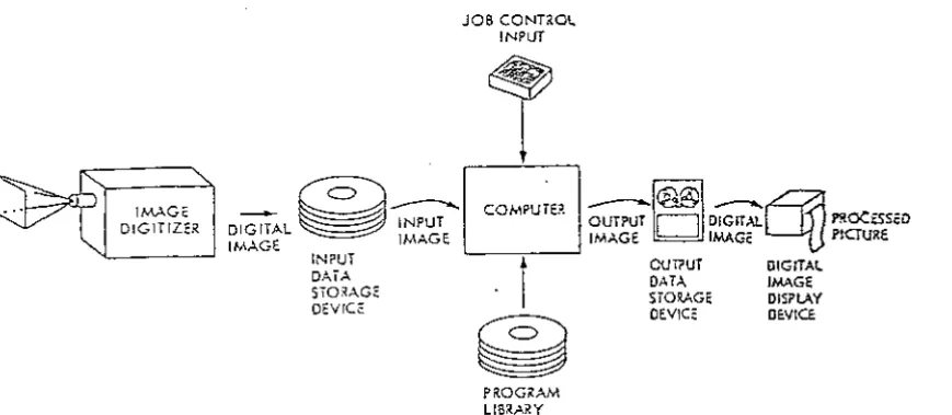
Figure 1-1 shows a complete system for image processing. The digital image produced by the digitizer goes into temporary storage on a suitable device. In response to job control input, the computer calls up and executes image processing programs from a library. During execution, the input image is read into the computer line by line. Operating upon one or several lines, the computer generates the output data storage device line by line. During the processing, the pixels may be modified at the programmer's discretion in processing steps limited only by his imagination, patience, and computing budget. After processing, the final product is displayed by a process that is the reverse of digitization. The grey level of each pixel is used to determine the brightness (or darkness) of the corresponding point on a display screen. The processed image is thereby made visible and hence amenable to human interpretation.

IMAGE DIGITIZER

JOB CONHOL

INPUT

1

___,... INPUT ourPur

D

DIGITAL no<:osco

DIGITAL IMAGE IMAGE IMAG- PICTURE

IMAGE c

~ [ COMM~

1~1@@1

~oTI

" - - - - ~ IN~UT l CUT?UT DIGITAL

DAIA

I

DATA IMAGE

STORAGe • STORAGE DISPLAY

oev,ce ~ oev,cs oev«:e

PROGRAM LIBRARY

Fig. 1-1 A digital image processing system

1.1.2 Basic Classes of Digital hnage Processing

Digital image processing has a broad spectrum of applications, such as remote sensing via satellites and other spacecraft, image transmission and storage for business applications, medical processing, radar, sonar, and acoustic image processing, robotics, and automated inspection of industrial parts.

Although there are many image processing applications, the basic classes of digital image processing are as follows:

* Image representation and modelling

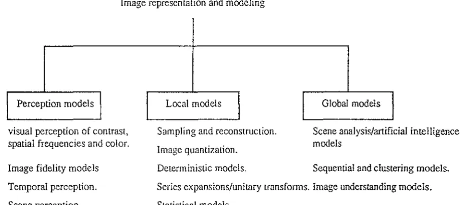
In image representation one is concerned with characterization of the quantity that each picture-element (also called pixel) represents. An image could represent luminance of objects in a scene (such as pictures taken by ordinary camera), the absorption characteristics of the body tissue (X-ray imaging), the radar cross section. of a target (radar imaging), the temperature profile of a region (infrared imaging). In general, any

[image:13.599.41.476.87.277.2]

dimensional function that bears information can be considered an image. Image models give a logical or quantitative description of the properties of this function. Figure 1-2 lists several image representation and modelling problems.

Image representation and modeling

Perception models

visual perception of contrast, spatial frequencies and color.

Image fidelity models

Temporal perception.

Scene perception.

Local models

Sampling and reconstruction.

Image quantization.

Deterministic models.

Global models

Scene analysis/artificial intelligence models

Sequential and clustering models.

Series expansions/unitary transforms. Image understanding models.

Statistical models.

Fig. 1-2 Image representation and modelling

* Image enhancement

In image enhancement, the goal is to accentuate certain image features for subsequent analysis or for image display. Examples includes contrast and edge enhancement, pseudocoloring, noise filtering, sharpening, and magnifying. Image enhancement is useful in feature extraction, image analysis, and visual information display. The enhancement process itself does not increase the inherent information content in the data. It simply emphasises certain specified image characteristics. Enhancement algorithms are generally interactive and application-dependent.

* Image restoration

Image restoration refers to removal or minimisation of known degradations in an image. This includes deblurring of images degraded by the limitations

[image:14.597.51.504.144.346.2]

of a sensor or its environment, noise filtering, and correction of geometric distortion or nonlinearities due to sensors.

* Image analysis

Image analysis is concerned with making quantitative measurements from an image to produce a description of it. In the simplest form, this task could be reading a label on a grocery item, sorting different parts on an assembly line, or measuring the size and orientation of blood cells in a medical image. More advanced image analysis systems measure quantitative information and use it to make a sophisticated decision, such as controlling the arm of a robot to move an object after identifying it or navigating an aircraft with the aid of images acquired along its trajectory.

Image analysis techniques require extraction of certain features that aid in the identification of the object. Segmentation techniques are used to isolate the desired object from the scene so that measurements can be made on it subsequently. Quantitative measurements of object features allow classification and description of the image.

* Image data compression

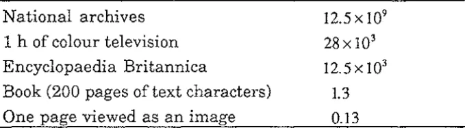
The amount of data associated with visual information is so large (see Table l. la) that its storage would require enormous storage capacity. Although the capacities of several storage media (Table l. lb) are substantial, their access speeds are usually inversely proportional to their capacity. Typical television images generate data rates exceeding 10 million bytes per second. There are other image sources that generate even higher data rates. Storage and/or bandwidth, which could be very expansive. Image data compression techniques are concerned with reduction of the number of bits required to store or transmit images without any appreciable loss of information. Image transmission applications are in broadcast television; remote sensing via satellite, aircraft, radar, or sonar; teleconferencing; computer communications; and facsimile transmission. Image storage is required most commonly for educational and business documents, medical images used in patient monitoring systems, and the like. Because of their wide

applications, data compression 1s of great importance 1n digital image processing.

Table l.la Data Volumes of Image Sources (in Millions of Bytes)

National archives 1 h of colour television Encyclopaedia Britannica

Book (200 pages of text characters) One page viewed as an image

Table 1.lb Storage Capacities (in Millions ofBytes)

Human brain Magnetic cartridge Optical disc memory Magnetic disc

2400-ft magnetic tape Floppy disc

Solid-state memory modules

* Image reconstruction from projections

12.5x 109

28x 103

12.5x 103

1.3 0.13 125,000,000 250,000 12,500

760

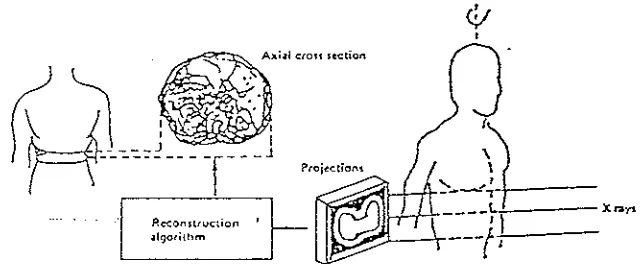
200 1.25 0.25

Image reconstruction from projections is a special class of image restoration problems where a two (or higher) dimensional object is reconstructed from several one-dimensional projections. Each projection is obtained by projecting a parallel X ray (or other penetrating radiation) beam through the object (Figure 1-3). Planar projections are thus obtained by viewing the object from many different angles. Reconstruction algorithms derive an image of a thin axial slice of the object, giving an inside view otherwise unobtainable without performing extensive surgery. Such technique is referred to as computerized tomography; it has revolutionized diagnostic radiology over the past decade. The 1979 Nobel prize in medicine has been awarded for work on computerized tomography. The fundamentals of computerized tomography will be introduced in the next section.

[image:16.600.113.453.147.240.2]

P.~onttruction '

-algorithm

<!I

_I

:k

'

,,

---·L...l.~----.,.-

_----r,

.Xnyi

~~-,----t

l

Fig. 1-3 Image reconstruction using x-ray CT scanners.

1.2. The Fundamentals of Computerized Tomography

We know that x- rays, radioisotopes, ultrasound and magnetic resonance can be used to obtain a reconstructed image. Because x-rays are broadly used today, we will only discuss utilizing x-rays to form the images based on their attenuation coefficient.

On November 1895, Professor Rontgen discovered the x-rays. The prospects for x-ray diagnosis were immediately recognised. In Great Britain, it has been estimated that there are 644 medical and dental radiography examinations per 1000 population per year, so that the technique is of major importance in medical imaging.

The radiographic image is formed by the interaction of x-ray photons with a photon detector and is therefore a distribution of those photons which are transmitted through the patient and are recorded by the detector. These photons can either be primary photons, which have passed through the patient without interacting or secondary photons, which result from an interaction in the patient. The secondary photons will in general be deflected from their original direction and carry little useful information. The primary photons do carry useful information. They give a measure of the probability that a photon will pass through the patient without interacting and this probability will itself depend upon the sum of the x-ray attenuating properties of all the tissues the photon traverses. The image is therefore a projection of the attenuating properties of all the tissues along the paths of the x-rays.

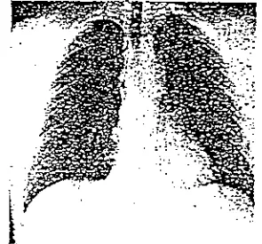
[image:17.596.114.434.75.207.2]

[image:18.597.168.316.168.306.2]

When we look at a chest x-ray (see Figure 1-4), certain anatomical features are immediately apparent. The ribs, for example, show up as a light structure because they attenuate the x-ray beam more strongly than the surrounding soft tissue, so the film receives less exposure in the shadow of the bone. Correspondingly, the air-filled lungs show up as darker regions.

Fig. 1-4 Typical chest x-ray radiograph

X-ray films usually allow contrasts of the order of 2% to be seen easily, so a 1 cm thick rib or a 1 cm diameter air-filled trachea can be visualised. However, the blood in the blood vessels and other soft-tissue details, such as details of the heart anatomy, cannot be seen on a conventional radiograph. In order to make the blood vessels visible, the blood has to be infiltrated with a liquid contrast medium containing iodine compounds; the iodine temporarily increases the linear attenuation coefficient of the fluid medium to the point where visual contrast is generated. Consideration of photon scatter further degrades contrast.

Another problem with the conventional radiograph is the loss of depth information. The three-dimensional structure of the body has been collapsed, or projected, onto a two-dimensional film.

It is apparent that conventional x-radiographs are inadequate in these two respects, namely the inability to distinguish soft tissue and the inability to resolve spatially structures along the direction of x-ray propagation.

The announcement of a machine used to perform x-ray computerized tomography (CT) in a clinical environment, by Hounsfield at the 1972 British

Institute of Radiology annual conference, has been described as the greatest step forward in radiology since Rontgen's discovery. The relevant abstract (Ambrose and Hounsfield 1972) together with the announcement entitled 'X-ray diagnosis peers inside the brain' in the New Scientist (27 April 1972) can be regarded as the foundation of clinical x-ray CT. Hounsfield shared the 1979 Nobel Prize for Physiology and Medicine with Cormack.

With computerized tomography, the two inabilities of conventional x-radiographs can be solved. By combining "ordinary" x-ray technology with sophisticated computer signal processing, computerized tomography can generate a display of the tissues of the body which is unencumbered by the shadows of other organs. Computerized tomography also passes x-rays through the body of a patient, but the detection method is usually electronic in nature, and the data is then converted from an analogue signal to digital impulses in an analogue-to-digital (A/D) converter. This digital representation of the x-ray intensity is fed into a computer, which then reconstructs an image.

Since Hounsfield's invention of the computerized tomography (CT) scanner in 1972, great improvements have been made in x-ray tomography, with the result that the patient scan time has been reduced to less than 10s from over 4 m1ns.

1.2.1. Theoretical Background for Image Reconstruction

1.2.1.1. The N-Dimensional Continuous Fourier Transform (CFT)

We consider here a function _{f(xpx2, ... ,xN)} of N continuous variables

Xi,X₂, ••• ,xN. We will generally find it convenient to express the N-tuple

(xi,x2, ... ,xN) as a vector

x

and refer to the function as

/(x).

The N-dimensional Fourier transform of f(x) is denoted by F(OJpOJ_{2, ••. ,0JN)} or F(w). The domain of

f(x) will be referred to as signal space and the domain of F(w) as Fourier space. The N-dimensional function /Ci) and its Fourier transform are related by:

+oo +oo

F(mpm2, ... , mN)

=

J ... J

f(xi,x2, ... ,xN )exp[-_j(m1x1

+

_{m2x2+ ... +mNxN )]dx1dx2 ... dxN}

or, expressed in vector notation,

and

+oo

F(iiJ)=

f

J(x)exp[-J(.x•w)]dx

f(x)

=

l

NT

F(m)exp[j(.x · w)]dm

(2n) _-oo

(1.1)

(1.2)

(1.3)

(1.4)

where

.x •

iiJ denotes the dot product of the vectors

x

and

w

or equivalently with

.x

and

m

interpreted as row matrices .x ·

m

=

.xw'.

A useful property of the N-dimensional Fourier transform pair which we will want to use later is that if f(x) and F(m) form a Fourier transform pair, then f(xA) and F(wA) form a Fourier transform pair if A is an orthogonal

t .

.

A-I A--1 ma nx, 1.e.,

=

.

This property is easily verified by direct substitution into (1.3). Thus an orthogonal transformation or equivalently an orthogonal change of coordinates in signal space results in the same change of coordinates in Fourier space. For example, for N=2, if

[

cose

sine]

A=

-sine

cose (1.5)

so that JCi) is rotated by an angle 0, then its Fourier transform will be rotated by the same angle 0.

1.2.1.2. The N-Dimensional Discrete Fornier Transform (DFT)

We are here interested in functions which can be processed by a digital computer and consequently can be represented by their samples. Thus we consider the class of band-limited functions. Specifically, JCi) is said to be band-limited if there exists an N-tuple (Wi,W_{2 , •••} ,WN) such that F(m) is zero

for

lm;I

> Wi> i

=

1,2, ... ,N. In some cases it is convenient to set

W

=

max(Wi, W_{2 , ••• ,} WN) and refer to the scalar Was the bandwidth of f(x).

The N-dimensional sampling theorem states that if f(x) is sampled in signal space on a rectangular lattice with the sample spacing in dimension X; less than TC I Wi, then f (x) can be recovered from its samples. Sampling on a

rectangular lattice will be referred to as periodic Cartesian sampling.

Let us denote by g(n) the N-dimensional sequence corresponding to sampling

f (x) with a sample spacing of TC I Vi in the dimension xi where Vi > Wi so that

(1.6)

from the sampling theorem the Fourier transform F(m) of f(x) can be obtained from g(n) by the relation

(1.7)

h - d h ( co1 CO2 wN ) d

w ere COv enotes t e vector - , - , ... , - an

v1 v2

vN

b y(CO) --{ 1,

lmil<Vi,

i=l,2, ... ,N

0, otherwise

likewise, the sequence g(n) can be obtained from F(m) by the relation

+V

g(n)

=

l N

f

F(w)exp{jn(n · Q)y )}dw (27r) -V

(1.8)

The original N-dimensional function f(x) can be obtained from the sequence g(n) by means of the interpolation formula

where

+oo

f(x)

=

I:gCn)</JCn,x)

n=-oo

sin V. (x. - nin)

</J(n,x)

=

IT . .

vi

i=l V.(x.-nin)

l l

v.

l

(1.9)

(1.10)

When only a finite number of the samples of f(x) are nonzero, the Fourier transform F(w) can be represented by a finite set of Cartesian samples. The relationship between the Cartesian samples of F(w) and the Cartesian samples of f(x) is the N-dimensional DFT. Specifically, let us assume that

g(n) = 0, if ni ~ Mi or ni < 0, i = 1,2, ... ,N.

We now consider the Cartesian samples of F(w), which we denote by G(k)

given by

where k; is an integer such that

M. M.

-1

+

1 ~ ki ~ - 1

, if M; is even

2 2

- Mi - l < k. < Mi - l if M

1

. is odd

2 - l - 2 '

Then

and

( ) - 1 ~ ~Gk~ . ~~ ~~

4~

g

n,,,~, ...

,nN - - - L . , ; · · · L . , ; ( i,"'2,···,kN)•exp[J2n(-+-+ ... + - - ) ]

M1 ·Mz · ... ·MN k1 k2 M1 Mz MN (1.12)

Since G(ki,k_{2 , •••} ,kN) as defined in (1.11) is periodic in k; it is frequently convenient to use the values of k; in the range given above. Adopting this

convention and defining the vector kM as the N-tuple

we can express (1.11) and (1.12) as

M-1

G(k)

=

L

g(n) · exp[-j2n(n · kM )] (1.13)

n=O

and

(1.14)

Equation (1.13) and (1.14) are referred to as the N-dimensional DFT pair. The N-dimensional DFT can be computed efficiently by using the one-dimensional fast Fourier transform (FFT) algorithm, since the summations in (1.13) and (1.14) can each be decomposed as a cascade of one-dimensional transforms.

The class of functions f (x) which can be represented by a finite number of samples will be referred to as band-limited functions of finite order M where

1.2.1.3. Projections

A projection is a mapping of an N-dimensional function to an

(N-1)-dimensional function obtained by integrating the function in a particular direction. For example, Px

2 (x1) given by

+=

px₂ (x,)

=

f

_f(Xi,X2)dx₂ (1.15)

is an example of a projection of the two-dimensional function _f(xi,x2) onto one dimension.

For the general case, we define a projection as follows: Let f(x) denote an N-dimensional function and let i1 denote a new set of coordinates where

x=ilA

and A is an orthogonal transformation. Then a projection onto the hyperplane (upu2, ... ,u;_pu;+i,···,uN) is defined as

+=

Pu; (llpU2,···,Ll;_pU;+i, ... ,uN)

=

I

f(uA)du; (1.16)

The coordinate axis u;, which is normal to the hyperplane onto which f(x) is

projected, will be referred to as the projection axis.

For N =2, the matrix A is given by

[

cos

e

sine] A=

-sin 0 cos0

In this case, the Ui, Uz coordinate axes are offset from the (x1,x2 ) axes by an angle of 0. For two-dimensional functions it will generally be convenient to

refer to a projection by its angle 0. A projection at angle 0 will be interpreted

to mean a projection onto the coordinate ½, which is at an angle 0 with x₁• Equivalently, then, the projection axis Uz is at an angle 0 to the coordinate axis x_{2 •} Equation (1.15) corresponds to a projection at an angle 0

=

0 or equivalently with x2 as the projection axis.

1.2.1.4. The Projection-Slice Theorem

The projection-slice theorem relates the (N-1)-dimensional Fourier transforms of the projections to the N-dimensional Fourier transform of the original function. Basically, the theorem states that the (N-1)-dimensional Fourier transform of a projection is a "slice" through the N-dimensional Fourier transform of f (x).

First, let us consider a projection for which the projection axis is one of the coordinate axes of f(x), for example, x_{1 •} Then px

1 (x2 , ••• ,xN) is given by

+=

Pxl (Xz,···,XN)

=

f

f(x)dx1 (1.17)

and its (N-1)-dimensional Fourier transform is given by

+oo +oo

Px, (OJz,···, (J)N)

=

J ...

f

Px, (Xz,···,XN). exp[-j(OJ2X2+ ... +WNXN )] (1.18)

Comparing (1.18) and (1.1), we see that

(1.19)

In other words, Px

1 (OJ2 , ... ,0JN) is a "slice" of F(wpw2, ... ,wN) defined by OJ1 =0.

Clearly, a projection whose axis is any coordinate axis xi has a Fourier transform that is a slice of F( OJ1> OJ_{2 , ••• ,} OJ N) defined by OJi

=

0.

A general projection was defined in (1.16) where A is an orthogonal transformation. It was argued previously that if F(w) is the Fourier transform of f(x) then F(Q) is the Fourier transform of /(u) where

(1.20)

From this, (19) is easily generalized to state that a projection for which the projection axis is the transformed coordinate ui has an (N-1)-dimensional

Fourier transform which is a slice of F(Q) for Qi

=

0 where the coordinate

systems

u

and Q are related to the coordinate systems

x

and

m

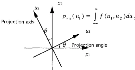
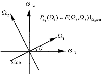
by the same orthogonal transformation. In two dimensions, for example, the projection-slice theorem states that the one-dimensional Fourier transform of a projection at an angle 0 is a slice at the same angle of the two-dimensional Fourier transform of the original object. This relationship is depicted in Figure 1-5.

X2

U2

Projection axis

UI

[image:26.599.121.384.364.501.2]

(I) 2

Fig. 1-5 The relationship between the projection of a two-dimensional function and slice of its Fourier transform.

1.2.1.5. The Basis for Reconstruction from Projections

From the projection-slice theorem, we see that specification of a projection in signal space corresponds to the specification of a slice in Fourier space and thus represents a partial specification of the signal itself. In principle, then, if an unlimited number of projections at different orientations are available, the Fourier transform of f(x) can be obtained and therefore so can f(x) itself.

Generally, in any practical context, we are restricted to a finite number of projections.

Under certain assumptions, it is possible to carry out an exact reconstruction from a finite number of projections. If the structure is highly symmetrical, a finite number of projections might suffice for exact reconstruction. For example, for a two-dimensional circularly symmetric function all of its projections are identical and consequently such a function can be represented exactly by a single projection. Similarly, in three dimensions, for an object which is cylindrically symmetric all of the projections for which the axis is normal to the longitudinal axis are identical and consequently, in this case also, a single projection is sufficient.

In uitilizing projections for reconstruction, many of the algorithms involve computing the Fourier transforms of the projections. The Fourier transform

[image:27.597.185.380.62.205.2]

of each projection is a function of a set of continuous variables, but only a finite number of points from each Fourier transform can be computed and stored. Thus from the projections, only samples in the Fourier domain are available, in part because of the limited number of projections and in part because only samples of the Fourier transform on each slice can be obtained. The essence of the reconstruction problem, then, is to approximate all of Fourier space from its values on a discrete point set.

1.2.1.6. Reduction of the Dimensionality of the Reconstruction Problem

As we saw in Section 4, the underlying basis for reconstruction is to obtain samples in the Fourier plane by transforming projections. Intuitively it seems reasonable that projections need not be taken in all orientations. For three-dimensional objects, for example, we could imagine using only projections in the spatial domain on planes parallel to one of the coordinates axis, say x1 • Slices of these projections at x1

=

A are then projections of the two-dimensional function f(A,x₂,xJ and, consequently, a two-dimensional

reconstruction algorithm can be applied to reconstructing this two-dimensional slice of the two-dimensional object. In this way, the dimensional object can be built up slice by slice and, consequently, the three-dimensional problem can be reduced to a series of two-three-dimensional problems. In the general case, we can apply a similar argument to reduce an N-dimensional problem to a set of (N-1)-dimensional problems each of which can in principle be reduced to an (N-2)-dimensional problem, etc.

Thus in principle, an N-dimensional problem can be reduced to a set of two-dimensional problems. Often this procedure requires considerably less storage and is simpler computationally than solving the N-dimensional problem directly. Furthermore, in many cases, we may be content with very coarse sampling in one or several dimensions. For the three-dimensional problem, for example, reconstruction of only a few slices may be sufficient.