Dynamic inversion of underactuated systems via squaring transformation matrix

(1)

Rochester Institute of Technology

RIT Scholar Works

Theses Thesis/Dissertation Collections

11-1-2007

Dynamic inversion of underactuated systems via

squaring transformation matrix

Ryan Schkoda

Follow this and additional works at:http://scholarworks.rit.edu/theses

This Thesis is brought to you for free and open access by the Thesis/Dissertation Collections at RIT Scholar Works. It has been accepted for inclusion in Theses by an authorized administrator of RIT Scholar Works. For more information, please [email protected].

Recommended Citation

(2)

Dynamic Inversion of Underactuated Systems Via

Squaring Transformation Matrix

By

Ryan F. Schkoda

A Thesis Submitted in Partial Fulfillment of the Requirement for Master of Science in Mechanical Engineering

Approved by:

Dr. Agamemnon Crassidis – Thesis Advisor

Department of Mechanical Engineering

Dr. Steve Weinstein

Dr. Mark Kempski

Dr. Edward Hensel

Department Head of Mechanical Engineering

Department of Mechanical Engineering Rochester Institute of Technology

(3)

PERMISSION TO REPRODUCE THE THESIS

Dynamic Inversion of Underactuated Systems Via

Squaring Transformation Matrix

I, RYAN F. SCHKODA, hereby grant permission to the Wallace Memorial Library of Rochester Institute of Technology to reproduce my thesis in the whole or part. Any reproduction will not be for commercial use or profit.

Date: Signature:

(4)

Abstract

(5)

Acknowledgments

(6)

List of Figures

2.1 Example of a 2-D phase portrait . . . 8

2.2 Concepts of stability . . . 9

2.3 Sliding surface behavior . . . 14

2.4 Linear vs. Nonlinear Response: 0.1 Deg Defelction . . . 37

3.1 Two-Mass System Schematic . . . 42

3.2 Tracking Response: Moore-Penrose . . . 43

3.3 Tracking Response: State One . . . 44

3.4 Control effort expenditures: State One . . . 45

3.5 Tracking Response: State Three . . . 46

3.6 Control effort expenditures: State Three . . . 47

3.7 Tracking Response: Moore-Penrose . . . 49

3.8 Tracking Response: State One . . . 50

3.9 Control effort expenditures: State One . . . 51

3.10 Tracking Response: State Two . . . 52

3.11 Control effort expenditures: State Two . . . 53

3.12 Tracking Response: State Four . . . 55

(9)

List of Tables

2.1 Solution Summary . . . 32

3.1 Dynamic coefficients and eigenvalues: State One . . . 45

3.2 Dynamic coefficients and eigenvalues: State Three . . . 48

3.3 Dynamic coefficients and eigenvalues: State One . . . 51

3.4 Dynamic coefficients and eigenvalues: State Two . . . 54

(10)

Nomenclature

A System Dynamic Matrix

B Input Influence Matrix

B† _{Moore-Penrose pseudoinverse of}_B

C Output Matrix

x State Vector

T Transformation Matrix

T∗ Alternate form of Transformation Matrix

Q State Weighting Matrix

R Input Weighting Matrix

s Sliding Surface

λ Positive Constant

λ Lagrange Multiplier (Section 2.3)

u Control Input

y Transformed State Vector

J Cost Function

K(t) Solution to Linear Quadratic Regulator

K Steady-State Solution to Linear Quadratic Regulator

Vt True Velocity

α Angle of Attack

p Roll Rate

q Pitch Rate

r Yaw Rate

φ Roll/Bank Angle

θ Pitch Angle

ψ Yaw/Heading Angle

V(x) Lyapunov Function (of variable x)

xd Subscript (d) denotes desired value (i.e. desired value of x)

˜

(11)

n System Order/Number of States

m Number of Inputs

p Number of Outputs

H Hamiltonian

S(t) Solution to the Riccati equation

S(∞) Steady-State Solution to the Riccati equation

sr Characteristic Root

j Unknown matrix that is to be determined

S(tf) Final state weighting matrix for the LQR problem (Section 2.3.1)

FAx, FAy &FAz Aerodynamic forces along the aircraft body-axis

FTx, FTy & TAz Thrust forces along the aircraft body-axis

Mex, Mey &Mez External applied moments about the aircraft body-axis

(12)

Chapter 1

Introduction

1.1

Background

Classical linear control architectures such as proportional, proportional-integral (PI) and proportional-integral-derivative (PID) are powerful techniques for controlling a wide range of systems. However, with the advent of more complex and nonlinear systems there is a need for more advanced control schemes capable of controlling such systems.

The development of state-space methods is perhaps one of the greatest advances in the controls community in the past sixty years. The defining characteristic of the state-space form is the resulting mathematical system model is a system of first-order differential equations rather than higher-order differential equations characteristic of transfer func-tion analysis. Individuals such as Professor Solomon Lefschetz, Professor J.R. Ragazzini, R.E. Kalman and J.E. Bertram among others as well as many scientists from the Soviet Union were responsible for bringing state-space methods to the forefront in the late 1950s and early 1960s [1].

Not only did state-space methods provide a different way of analyzing dynamical systems but numerical techniques were available to approximate the time history response of a system in state-space form. Numerical integration techniques such as the Euler and Runge-Kutta methods are particularly well suited to approximate the solution of a system in state-space form. Also, the introduction of digital computers further progressed calculation of these solutions. With out the aid of digital computers, solving a state-space model would be nothing more than an academic exercise.

(13)

1.2

Current Work

Non-square systems are common in nature as well as in engineering practice. If fact, when modeling systems in the “real world,” square systems may form the minority. For a system to be square the number of inputs must equal the system order. This is a completely arbitrary constraint and is rarely satisfied. Certain control architectures indirectly rely on a system being square. One such control architecture is sliding mode control. The development of a sliding controller requires an inversion of the system’s input influence matrix (B). If the system is non-square, the input influence matrix is singular and not invertible. There have been numerous attempts documented in literature to design viable control schemes for non-square systems. Most all of these schemes revolve around dynamic inversion based controllers.

After performing a literature review it became clear that topic of this thesis is a fairly novel idea. There is much literature concerning the control of non-square systems but a lack of literature related to the method being proposed in this thesis.

An automobile constitutes a non-square system. In a paper by Wang and Longoria [2] the problem of controlling vehicle chassis is investigated. Control inputs include wheel torque and steering actuation. A two stage control system is developed. Stage one involves developing a sliding controller to produce general forces and moments necessary and to control the vehicle and stage two utilizes a weighted pseudoinverse to determine control allocation. (For an definition and discussion on pseudoinverses and a weighted pseudoinverse see Section 2.5)

Non-square systems are also found in biological systems such as the muscular sys-tem designed to control and coordinate eye movement. A paper authored by Dean and Porrill [3] notes this problem of redundancy in both robotic and biological systems. For the control of oculomotor systems the authors use a PID controller utilizing a weighted pseudoinverse. Because eye movement is controlled by several thousand muscular actu-ators the basic control solution is not unique [3]. Once again a particular solution must be determined with the aid of the pseudoinverse.

(14)

[5].

In the closely related field of unmanned or uninhabited air vehicles (UAVs) the prob-lem of controlling non-square systems is addressed. Papers by Boskovic et al [6], Haitao & Jinyuan [7] and Boskovic & Mehra [8] all address the issue of tracking control for non-square aircraft models. All of these papers make use the weighted pseudoinverse to address the issue of control allocation. Boskovic et al seek to develop a weighting matrix such that it does not saturate the control surface actuators [6]. This weighting matrix is then used to form the pseudoinverse which in turn defines the control allocation. Haitao and Jinyuan proposed a control architecture utilizing traditional aircraft equations of motion, nonlinear mapping and a single hidden layer (SHL) neural network [7]. Once again the pseudoinverse is used to define control allocation. The pseudoinverse is defined such that it minimizes control energy. The paper by Boskovic and Mehra specifically addresses the issue of control allocation under position and rate limiting. The authors seek to find a more effective way of determine optimal and satisfactory control allocation. In yet another application regime of underwater vehicles the problem of controlling non-square systems has been addressed. Papers by Omerdic et al [9] and Fossen & Johansen [10] specifically address the issue of control allocation. Both these papers assume the systems are overactuated and examine ways to efficiently control the craft based on certain criteria. Omerdic et al adapt a standard pseudoinverse method by combining it with a fixed-point iteration method. Fossen & Johansen produced a paper that was meant to be a survey of control allocation methods available for underwater vehicles. In section III there is specific reference to the generalized inverse and its relation to the Moore-Penrose pseudoinverse [10]. A derivation of Moore-Penrose using Lagrange multipliers is presented.

(15)

The general form of the nonlinear structural systems examined here is restricted to

¨

x=N(x,x˙) +BU (1.1)

wherex, ˙x,¨xare n×1 vectors of generalized coordinates and their first and second deriva-tives, respectively; N(x,x˙) is an n×1 vector of nonlinear functions; B is an (m+ 1)×1 matrix of control input weighting coefficients and U is a scalar.

The state vector is

xT _{= [}_{θ, q}

1, . . . , qm] (1.2)

whereθis the hub rotation (Parker’s work dealt with mechanical rotation) andq1 through qm represent the remaining states. Therefore, there is one rotational equation of motion

that can be extracted from Eq. (1.1) is

¨

θ =N1+B1U (1.3)

where N1 is the nonlinear rigid body equation of motion and B1 is the input gain.

Equation (1.3) is a scalar equation with U as the input and ¨θ as the output. However,

N1 is a nonlinear equation involving the remaining states.

Following from this the sliding surface may be chosen as

s=wθe+ ˜wTq_e

+θ˙e+ ˜wTq˙_e

= 0

θe≡θ−θref (1.4)

q_e ≡q−q_ref

Where wis a constant and ˜w is a 1×m vector of weighting coefficients. By defining the sliding surface as it has been defined in Eq. (1.4) it becomes a scalar equation where the dynamic variable is not state error (as it is in SMC) but a weighted sum of all the state errors. Now that both equations are in scalar form, the derivative of Eq. (1.4) may be taken and substituted into Eq. (1.3) to form the control law

B1U =−w

˙

θe+ ˜wTq˙_e

−N1+ ¨θref −w˜T¨q_e (1.5)

The remaining problem is to determine the form of the constant wand the vector ˜w. System performance will be defined by a nonlinear cost function J. The parameters w

and ˜w will be determined such that they minimize the cost function J as well as satisfy any other constraints.

(16)

The author assumes the state-space model is as follows

˙

x=Ax+Bu

y=Cx+Du (1.6)

It is desired to regulate the system with

u=−Ex (1.7)

where E is a constant feedback gain matrix of the form

E= (CB)−1_j _(1.8)

Wherejis an arbitrary diagonal matrix with specified eigenvalues. If the system outputs are defined as they are in Eq. (1.6) and the dimension of yis not equal to the dimension of x then the input-output relationship is non-square and the product CB in Eq. (1.8) cannot be inverted. El Singaby’s paper presents a method of redefining C as Csq such that the product CsqB is square and invertible.

The results reached by El Singaby are interesting because they are similar to the results developed in this thesis and reminiscent of the pseudoinverse. Throughout this thesis it is assumed that the states of the system are available or can be estimated with a high degree of certainty. This implies theCmatrix is identity. The El Singaby paper does not make this assumption. Cases where there are fewer outputs then inputs (p < m) and more outputs then inputs (p > m) are addressed. In the case where p < m the system needs to be “squared up,” while for p > mthe system needs to be “squared down.”

Although El Singaby’s paper proposes a matrix j responsible for closed loop pole placement there is no proposed method for choosing the matrix. Also, El Singaby’s paper does not attempt to track any desired states. The idea of squaring a system was investigated only for the purpose of the regulation, not tracking.

Additional methods for designing control schemes for overactuated models can be seen in Bakaric et al [13], Johansen [14] and Oppenheimer [15].

1.3

Overview and Motivation for Present Work

(17)

may be developed by using what is known as a generalized inverse or pseudoinverse. However, the pseudoinverse is not unique and may not provide satisfactory results due to its form. By studying the problem and understanding the mathematics it may be possible to develop a satisfactory sliding controller despite the requirement of inverting a singular matrix.

The development and analysis of such a controller was done first by theoretical math-ematical development then simulation in SimulinkR

and analysis in MATLABR

. The general structure for the research was as follows:

1. Develop a theoretical solution to overcome the difficulty of inverting a singular matrix

2. Simulate the dynamical response when the proposed control law is implemented

3. Analyze system properties of a closed-loop system

(18)

Chapter 2

Theoretical Development

2.1

Lyapunov Theory

Preface

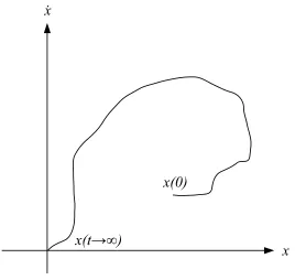
When analyzing linear systems Laplace transforms and eigenstructure analysis can offer much insight into the stability of a system. However, Laplace transforms and eigen-structure analysis are not applicable when the system being analyzed is nonlinear. For nonlinear system analysis the theory developed by Aleksandr Mikhailovich Lyapunov is extremely useful. Some of Lyapunov’s work concerning nonlinear system stability can be more easily understood by examining the system’s phase portrait (For an exapmple see Figure 2.1). Because each axis of a phase plane corresponds to a system state, the trace of the system states as the system propagates offers some insight as to the stability of the system. If for some initial condition x(0) the state trajectories either remain in the vicinity of their initial location or tend toward the origin they are thought of as being well behaved, or stable. Conversely, if for some initial condition x(0) the state trajectories tend toward infinity as the system propagates the system is unstable. The idea of phase plane behavior is used to characterize system stability.

2.1.1

Phase Portrait

(19)

trajectories of a system. Obviously, when physically constructing a phase portrait one is limited to three dimensions. However, a phase portrait may exist in any n-dimensional space.

[image:19.612.183.451.204.458.2]

Because the state variables define a dynamical system, their trajectories or behavior can offer insight to the character of the system. A phase portrait is a plot where each axis represents a state variable and the trace represents the time history response of the states.

Figure 2.1: Example of a 2-D phase portrait

Figure 2.1 displays an example of a 2-D phase portrait. The particular phase portrait describes a stable system where each state has some initial condition atx(0) and the final value of the states are at the origin, or 0. The trace defines the time history response of the state variable. The shape of the trace alone or the shape of the trace for various initial conditions may offer insight of system character.

2.1.2

Definitions of Stability

Consider the following form for a general nonlinear system

˙

(20)

wheref is an×1 nonlinear vector function, andxis then×1 state vector. The definitions of stability in a Lyapunov sense are presented in Slotine [16]. Theory concerning sliding mode control relies heavily on an understanding of stability based on Lyapunov stability. The following definitions and discussion is meant to introduce the idea of Lyapunov stability.

Definition 2.1. The equilibrium state x=0 is said to bestable if, for anyR >0, there

exists r > 0, such that if kx(0)k < r, then kx(t)k < R for all t ≥ 0. Otherwise, the equilibrium point is unstable.

∀R >0,∃r >0,kx(0)k< r⇒ ∀t≥0,kx(t)k< R

Definition 2.1 is perhaps the most basic definition concerning Lyapunov stability. Essentially, if the state trajectory is started arbitrarily close to an equilibrium point (defined by a ball with radius r), the state trajectory will stay in the vicinity of that equilibrium point (defined by a radius R). Figure 2.2 illustrates the idea of Lyapunov stability.

curve 1 - asymptotically stable curve 2 - marginally stable curve 3 - unstable

Figure 2.2: Concepts of stability

Definition 2.2. An equilibrium point 0 is asymptotically stable if it is stable, and if in

addition there exists some r >0 such that kx(0)k< r implies thatx(t)→0 ast → ∞.

(21)

a system is asymptotically stable there is some a priori knowledge of how the systems trajectories will propagate.

Definition 2.3. An equilibrium point 0isexponentially stableif there exists two strictly

positive numbers a and b such that

∀t >0,kx(t)k ≤akx(0)ke−bt

in some ball Br around the origin.

Definition 2.3 restricts Definition 2.1 even further by defining not only whetherx(t)→ 0 as t→ ∞ but howx(t)→0 as t→ ∞. If a system is determined to be exponentially stable its state trajectory is upper and lower bounded by akx(0)ke−bt_.

Definition 2.4. If asymptotic (or exponential) stability holds for any initial states, the

equilibrium point is said to be asymptotically (or exponentially) stablein the large. It is also called globally asymptotically (or exponentially) stable.

Definition 2.4 extends the definition of stability to include the entire surface for which the system is defined. The definitions presented prior to Definition 2.4 are all concerned with equilibrium points and assume x(0) is arbitrarily close the the equilibrium point. If a system is determined to be globally asymptotically (or exponentially) stable then

x(t)→0as t→ ∞ for any and all x(0).

The preceding definitions may now be used to define a Lyapunov function.

Definition 2.5. If, in a ballBR0, the functionV(x) is positive definite and has continuous

partial derivatives, and if its time derivative along any state trajectory of system (2.1) is negative semi-definite, i.e.

˙

V(x)≤0

then V(x) is said to be aLyapunov function for the system (2.1).

Theorem 2.6 (Local Stability). If, in a ball BR0, there exists a scalar function V(x)

with continuous first partial derivatives such that

• V(x) is positive definite (locally in BR0)

• V˙(x) is negative semi-definite (locally in BR0)

(22)

Theorem 2.6 may be extended to include the all possible state trajectories.

Theorem 2.7 (Global Stability). Assume that there exists a scalar function V of the

state x, with continuous first order derivatives such that

• V(x) is positive definite

• V˙(x) is negative definite

• V(x)→ ∞ as kxk → ∞

then the equilibrium at the origin is globally asymptotically stable.

The preceding definitions and theorems formalize the concept of stability from a Lya-punov standpoint. Linear systems have the advantage of possessing constant eigenvalues which offer information regarding system stability. Analysis based on Lyapunov theory allows for stability to be examined for nonlinear systems. The Lyapunov function V(x) will be utilized in the development of what is called a sliding surface in Section 2.2.

2.2

Sliding Mode Control

Preface

The concept of sliding mode control seeks to reduce the dynamics of a general system to an asymptotically stable differential equation where the dynamic variable is tracking error. The control architecture is particularly useful because of its ability to control nonlinear systems and is robust to parametric uncertainty. The controller is designed to produce favorable state tracking. The following section introduces the fundamentals of sliding mode control as presented in Slotine [16].

2.2.1

Sliding Surface

Sliding mode control centers around the concept of sliding surfaces. To illustrate the concept consider the following general system

x(n) =f(x) +b(x)u (2.2)

where the state vector x is defined as x = [x x˙ · · · x(n−1)_]T_{, the} _nth _{derivative of the}

(23)

is b(x) and the system input is u. The goal of the control scheme is to track a desired, time varying state vector defined as xd= [xd x˙d · · · x(

n−1)

d ]T.

Let the tracking error vector, ˜x, be defined as

˜

x=x−xd = [˜x x˙˜ · · · x˜(n−1)_]T _(2.3)

then define a time-varying surface, s(x;t), in the state-space, R(n)_{, by}

s(x;t) =

d dt +λ

(n−1)

˜

x (2.4)

and λ is a strictly positive constant.

If, for instance, n= 2 the sliding surface would be defined as

s(x;t) = ˙˜x+λx˜

or a weighted sum of all the state errors.

If the current state of the system satisfies s(x;t) = 0 then the error trajectories are said to be “on the sliding surface” and the error vector will approach zero according to the dynamics of the sliding surface. The situation is known as the “sliding phase.” Furthermore, if the condition

xd(0) =x(0) (2.5)

is satisfied then the error trajectories are at the origin and remain at the origin since the surface, s, is constructed such that the origin is Lyapunov stable (See Section 2.2.2).

In the event s(x;t)6= 0 the system is said to be in the “reaching phase.” If the error trajectories are not on the sliding surface it is necessary to show that they will tend toward the sliding surface. Section 2.2.2 addresses the solution to this potential problem utilizing Lyapunov stability.

Considering the preceding discussion it is clear that the sliding surface is both a place and a dynamic [16]. The method of sliding mode control develops a controller causing the closed loop dynamics to be that of the sliding surface; ensuring favorable tracking.

2.2.2

Surface Stability

(24)

s(x;t) = 0 whens(x;t)6= 0, and to stay ons(x;t) = 0 once on it, the candidate Lyapunov function is chosen to be

V(x) = 1 2s

2 _(2.6)

Conceptually, s(x;t) defines a surface in the state-space. The desired location on the surface is s(x;t) = 0 because once on s(x;t) = 0 the tracking error, ˜x, will tend toward zero according to Eq. (2.4). V(x) is related to thedistance froms(x;t) = 0. It is obvious that V(x) is positive definite due to the square term.1 _Since _V₍_x_{) is positive definite,}

whether or not the function is stable from a Lyapunov standpoint can be determined from Eq. (2.7)

1 2

d dts

2 _≤₀ _(2.7)

Satisfying Eq. (2.7) implies that regardless of the magnitude of s(x;t) it will not in-crease. However, this criteria is insufficient from a tracking standpoint. The magnitude of s(x;t) is related to the magnitude of the function forcing the dynamic error equation (Eq. (2.4)). The left hand side of Eq. (2.7) equaling zero implies the magnitude of s is neither increasing nor decreasing. In order for ˜x to be allowed to follow the dynamics associated with s(x;t) = 0 and to converge to zero the following condition is required [16].

1 2

d dts

2 _{≤ −}_η_|_s_| _(2.8)

Where η is a small positive constant. Satisfying Eq. (2.8) means the forcing function will approach zero allowing ˜x to converge to zero. Notice, however, that s(x;t) may be set equal to zero at t = 0 with proper selection of initial conditions. The simulations analyzed in this work made use of initial conditions that force s(x;t) equal to zero at

t= 0 and because of Eq. (2.7), s(x;t) will never stray from zero.

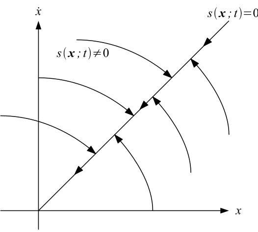
The implications of Eq. (2.6) and Eq. (2.8) can be visualized in Figure 2.3. The error trajectories will always point towards(x;t) = 0, and once ats(x;t) = 0, will tend toward the origin. What this means for sliding mode control is, once on the sliding surface, the overall state error will not increase. Furthermore, if there is no initial error (due to

xd(0) =x(0)) none is developed. Satisfying Eq. (2.6) and Eq. (2.8) is achieved through

proper controller development which is discussed in Section 2.2.3.

(25)

[image:25.612.184.447.68.305.2]

Figure 2.3: Sliding surface behavior

2.2.3

Controller Development

The objective of controller design is to develop a sliding controller so the closed loop system dynamics reduce to the sliding surface definition. The steps for designing a sliding controller are

1. Define a sliding surface

2. Set the sliding surface equal to zero and differentiate. Setting the surface equal to zero enforces the sliding condition; or, states the error trajectories will behave according to a stable, homogeneous differential equation. Differentiating the surface makes its order match that of the dynamic system so x(n) _{may be eliminated.}

3. Substitute the system dynamics into the equation of the differentiated sliding sur-face so as to eliminate x(n)

4. Solve for the control input, u

By defining a “sliding surface” and developing a control law utilizing the sliding surface the dynamics of a general state-space model can be transformed to

˙˜

(26)

or a stable differential equation where the dynamic variable is tracking error, x˜. If λ

is a positive constant then Eq. (2.9) inherently defines a stable, homogeneous ordinary differential equation. Because of its form the tracking error will asymptotically approach zero. Development of a control law satisfying Eq. (2.9) requires dynamic inversion of the input influence matrix.

The term sliding surface is meant to be more of a physical interpretation of the state trajectory on the phase plane. The sliding surface uses the tracking error vector as its dynamic variable and results in a trajectory that leads to the origin, or zero error. If the error is “placed” on the sliding surface, it will “slide” toward the origin, or toward zero error. Whether or not the error trajectories are on the sliding surface depend on the initial conditions and uncertainties contained in the system.

2.3

The Linear Quadratic Regulator

Preface

The Linear Quadratic Regulator (LQR) is a well documented and classic control prob-lem. The LQR problem is concerned with regulating a linear plant model subject to a quadratic cost function [17]. Generally, the form of the solution depends on the boundary conditions.

2.3.1

Final State Free Boundary Condition

When seeking to regulate a state-space model there are two popular sets of boundary conditions. The initial conditions are defined by x(0). The final state, x(tf), can either

be fixed or free. The final state being fixed implies at tf the states will be exactly at a

specified value. The optimal control problem develops a control law bringing the states to these specified values while minimizing the scalar cost function

J = 1

2 Z tf

to

uTRu dt

The final state being free implies the value of the states at tf is not predetermined.

However, the final values are incorporated into the cost function. As before, the optimal control problem seeks the most efficient way to control the system. Consider the linear time-varying plant

˙

(27)

where x∈ ℜn _and _u_{∈ ℜ}m _{with the associated quadratic cost function}

J = 1

2x

T₍_t

f)S(tf)x(tf) +

1 2

Z tf

to

(xTQx+uTRu)dt (2.10)

where S(tf)≥0 is the final state weighting matrix, Q≥0is the state weighting matrix

and R > 0 is the input weighting matrix. These matrices are generally diagonal so each diagonal element is a weighting factor. Off diagonal elements imply cross-coupling among weights. Cross-coupled weights is a fairly nonintuitive concept and are atypical in practice.

The method for determining a control effort, u, minimizing the cost function J is summarized as follows [17]:

1. Define the Hamiltonian, H

H(x,u, t) = (xTQx+uTRu) +λT(A(t)x+B(t)u−x˙)

where, in this section, λ, represents the Lagrange multiplier

2. Differentiate the Hamiltonian with respect to all variables,λ,xandu (resulting in the state equation, costate equation and stationary condition)

3. Enforce proper boundary conditions

4. Solve the Riccati equation

the result of this procedure is

u(t) =−R−1BTS(t)x(t)

where S(t) is the solution to the Riccati equation. The Kalman gain is defined as

K(t) =R−1BTS(t)

so

u(t) =−K(t)x(t)

(28)

2.3.2

The Steady-State Solution

As mentioned in section 2.3.1 the optimal control law for the LQR may be difficult to implement sinceK(t) is time varying. It is possible, in some instances, to replace the time varying gain matrix K(t) with a constant matrix K without significant loss controller performance.

Because the Riccati equation is solved backwards in time the final value of the solution is the initial value of K. Furthermore, for a stabilizable plant, there is always a positive semidefinite limiting solution to the Riccati equation [16].

Let

u=−Kx (2.11)

Where

K=K(∞) = R−1BTS(∞)

Note that Eq. (2.11) is the optimal control law for the infinite horizon LQR problem whose performance index is

J∞=

1 2

Z tf

to

(xTQx+uTRu)dt

Thus, as the final time approaches ∞ the use of the steady state control becomes more and more acceptable.

2.4

The Transform

The procedure developed in Section 2.2.3 requires an inversion of the input influence matrix. Depending on the system definition the input influence matrix may be singular and non-invertible. By introducing a transform and applying it to the original system it is possible to develop a sliding controller for the transformed system.

Consider the general State-Space model

˙

x=Ax+Bu (2.12)

where A∈ ℜn×n _and _B_{∈ ℜ}n×m_{. Define a sliding surface,}_s_{, as}

s=

d dt +λ

nZ t

0

˜

x dr

(29)

equations

s=x−xd+λ

Z t

0

(x−xd)dr (2.14)

Once the state trajectories are on the sliding surface no movement is ensured off the surface by taking the time derivative ofsand setting it equal to zero. Applying Leibniz’s rule

˙s=x˙ −x˙d+λ˜x= 0 (2.15)

substituting Eq. (2.12) into Eq. (2.15) and re-arranging:

u=B−1[x˙d−Ax−λx˜] (2.16)

If Eq. (2.16) is substituted into Eq. (2.12) the result is Eq. (2.9). As can be seen in Eq. (2.16) the control law developed via sliding mode control requires the inversion of the B matrix. If B is non-square and the pseudoinverse is used, certain dynamics may be lost and perfect tracking of all states may not be possible.

If B is invertible favorable control of all states is possible. If B is not invertible, however, then all the states may not be controlled simultaneously and the concept of

selectable states arises. The term selectable states refers to selecting which states will

have the most desirable behavior. The idea is to choose which states will be controlled most effectively at the expense of satisfactory control of remaining states. For instance, if B is not invertible and all the states cannot be controlled, is it possible to select some subset of statesxq ∈xn to be controlled more aggressively than the subset of remaining

states xn−q ∈xn?

We have noted the difficulties associated with controlling all states when B is not invertible. Instead, some combination of the states will be controlled. This is essen-tially a process of defining fictitious outputs where the mapping function is of “suitable” dimension as discussed in Section 6.4 of Friedland [1]. Define a mapping function, i.e.

y=Tx (2.17)

where T is a constant, fully populated m ×n matrix. Differentiating Eq. (2.17) and substituting into Eq. (2.12) results in

˙

(30)

Define a new sliding surface, s, as

s=

d dt +λ

nZ t

0

˜

y dr

(2.19)

Creating a surface for each equation in the state space system results in the system of equations

s=y−yd+λ

Z t

0

(y−yd)dr (2.20)

As before, once the state trajectories are on the sliding surface we ensure no movement off the surface by taking the time derivative of s and setting it equal to zero. Applying Leibniz’s rule

˙s=y˙ −y˙d+λ˜y= 0 (2.21)

where

˜

y=y−yd (2.22)

substituting Eq. (2.18) into Eq. (2.21) and re-arranging:

u= (TB)−1[y˙d−TAx−λy˜] (2.23)

or

u= (TB)−1T[x˙d−Ax−λx˜] (2.24)

Note the term requiring inversion is no longer B but TB. If T is chosen so that TB is non-singular an inversion of the resulting matrix is possible. If Eq. (2.23) is substituted into the system in Eq. (2.18) the closed loop system dynamics are similar to those in Eq. (2.9), but for the dynamic variable y

˙˜y+λy˜= 0 (2.25)

This form allows for proper inversion but poses the investigator with a new problem; what is the form of T?

2.5

The Pseudoinverse

Preface

(31)

may or may not contain properties associated with the true inverse. The pseudoinverse may be used in place of the true inverse at the expense of possibly unfavorable results.

2.5.1

Relation to the True Inverse

A pseudoinverse can be used to invert a singular matrix however, the results may be unfavorable. A non-singular matrix B has a unique inverse, denoted by B−1_{, such that}

BB−1 =B−1B=I (2.26)

Where Iis the identity matrix [18]. There are numerous properties of the inverse

(B−1)−1 = B

(BT)−1 = (B−1)T (B∗)−1 = (B−1)∗ (AB)−1 = B−1A−1

where BT and B∗ denote the transpose and conjugate transpose, respectively, of B. A matrix, B⋄, may be considered a pseudoinverse of a given matrix B if it

1. Exists for a class of matrices larger than the class of nonsingular matrices.

2. Has some of the properties of the true inverse

3. Reduces to the true inverse when B is non-singular

Because the definition of B⋄ _{is not extremely specific, a particular definition for a}

pseu-doinverse may not be unique. And while B⋄ may be designed to have certain properties of the true inverse, Eq. (2.26) is usually the most sought after.

2.5.2

Square, Overactuated and Underactuated Systems

(32)

Because the control architecture being investigated in this thesis requires full state feedback it is assumed the system outputs are the state variables. Therefore, the number of outputs equals the number of states (i.e p=n) or C=In×n.

Definition 2.8. A state-space model of the form x˙ = Ax+Bu is said to be square if

the number of inputs equals the number of outputs (i.e. m =p) and the columns of the

B matrix are linearly independent (i.e. B is invertible).

The term “square,” when referring to the shape of a system, indicates there are as many inputs, m, as there are outputs, p, or in this case states. In this thesis, the term “square” also implies the B matrix is invertible. The columns of B being linearly inde-pendent implies each input has indeinde-pendent, unique influence on the system. Intuitively this means none of the controllers need to be “shared.”

Definition 2.9. A state-space model of the formx˙ =Ax+Buis said to beoveractuated

if the number of inputs is greater than the number of outputs (i.e. m > p) and the rank of B is equal to n (i.e. R(B) =n)

The condition ofm > pamounts to theBmatrix being “fat” or “wide.” The condition

R(B) =n implies after the matrix has been put in row echelon form it will be a square matrix. The n independent columns of the B matrix represent n independent control inputs. All the columns eliminated via elementary row operations represent redundant or superfluous inputs. Becausem−ninputs are linearly dependent and may be removed without loss of control capability the system is considered overactuated.

It is common to encounter overactuated or redundantly actuated systems in practice. Any system that is responsible for human safety is typically overactuated. If a redundant control input is damaged or lost the system can still function properly. An example of such a system is the directional control of an aircraft. There are typically redundant control surfaces so that if one is damaged the aircraft may still be controlled.

Definition 2.10. A state-space model of the form x˙ =Ax+Bu is said to be

underac-tuated if the number of inputs is less than the number of outputs (i.e. m < p).

The condition ofm < p amounts to theB matrix being “tall.” There is no condition of the rank of B because if the columns are linearly dependent, the system will be underactuated so long as m < p. Underactuated systems represent a large portion of dynamical systems. Any single-input single-output (SISO) system with order > 1 and most single-input multiple-output (SIMO) systems are underactuated.

(33)

2.5.3

The Moore-Penrose Pseudoinverse

As noted in Section 2.5.1 the pseudoinverse of a given matrix is not unique and may be formed to posses certain properties. Consider, the linear systemAx=b. One would find the solution foex by formingx=A−1b assuming A−1 exists. In practice, however, one may encounter the situation whereAis non-square or singular. This should immediately inform the investigator the problem is poorly posed. Even so, it may be desired to form a solution x that minimizes the residual, r, defined bykb−Axk2. The Moore-Penrose

PseudoinverseofA, denotedA†_{, accomplishes this task. The form of the Moore-Penrose}

pseudoinverse is as follows [19]

B†=

(

BT(BBT)−1 _if _B _{has full row rank}

(BBT)−1_BT _if _B _{has full column rank} (2.27)

The following theorem and proof is from Cline [19].

Theorem 2.11. For any system of equations Ax = b where A has full column rank,

x=A†_b _{is the unique vector with} _k_b₋_Ax_k2 _minimal.

Proof. If A is square or if m > n and Ax = b is consistent, then with

A† = (ATA)−1_AT _{a left inverse of} _A _and _AA†_b₌_b_{, the vector}_x₌_A†_b _is

the unique solution with kb−Axk2 = 0. On the other hand, if m > n and

Ax=b is inconsistent,

kb−Axk2 = k(I−AA†)b−A(x−A†b)k2

= kb−AA†bk2+kA(x−A†b)k2

since AT(I−AA†_{) =} ₀_{. Hence} _k_b₋_Ax_k2 _{≥ k}_b₋_AA†_b_k2 _{where equality}

holds if and only ifkA(x−A†_b₎_k2 _{= 0. But}_A_{with full column rank implies}

kAyk2 ≥0 for any vector y6=0, in particular for y=x−A†_b

(34)

2.5.4

Relationship Between the Transform and the

Pseudoin-verse

Recall the similarities between the original sliding mode control law in Eq. (2.16)

u=B−1[x˙d−Ax−λx˜]

and the proposed sliding mode control law for the transformed system in Eq. (2.23)

u= (TB)−1T[x˙d−Ax−λx˜]

The significant difference between Eq. (2.16) and Eq. (2.23) is B−1 appears to have been replaced by (TB)−1_T_{. This is an interesting result since (}_TB₎−1_T_{will produce a matrix}

whose dimensions are opposite that of B. Furthermore, if T=BT then (TB)−1_T _{is the}

Moore-Penrose inverse.

By defining fictitious outputs, or by applying a squaring transformation matrix to the original system we have proposed a problem that amounts to defining a new pseudoin-verse. It is desired that this new pseudoinverse, defined by the matrix T will have the property that it maintains the sliding mode error equations for the fictitious outputs, as in Eq. (2.25), while minimizing the LQR cost function in terms of state trajectories and control effort.

2.6

Dynamic Extension

Preface

(35)

system is no longer in state-space form.

2.6.1

Concept

Dynamic Extension is a method for accommodating a non-square input influence matrix. By differentiating the system equations the derivative of the original input is present. By substituting the new set of equations into the original ones it is possible to, effectively, square the system [16]. Consider the following 2-state system where theAandBmatrices are not functions of time.

˙

x=A2×2x+B2×1u (2.28)

By performing dynamic extension, it is possible to obtain the system into the following form

¨

x=A′₂_×₂x+B′₂_×₂

"

u

˙

u

#

(2.29)

where the prime symbols indicate that the numerical values of the matrix may have changed. Note, the system in Eq. (2.29) is now square and an inversion of Bis possible. Also, the square system is no longer in standard state-space form; the second derivative of the state vector is on the left hand side of the equation rather than the first derivative. This method has a number of shortcomings. While there is a general procedure for performing dynamic extension there is no general form of the solution. The system equations must be manipulated individually for each different system. While this is mainly differentiation and algebra, the implementation is tedious for systems with more than three states.

Results of this method will not be presented. Because the resulting system may be invertible, the sliding controller will be able to provide perfect tracking. The drawback to this method is not its inability to provide satisfactory tracking, it is the difficulty in performing the method. Appendix A shows the necessary work to transform a 4-state system with one input into a square system.

2.6.2

Effects of the Method

Notice dynamic extension is not a control methodology. It is merely a method to square a system. Once a system has has dynamic extension applied to it, the task of developing the control law remains.

(36)

being transformed into a second order (non state-space) model. The effect of this trans-formation is the addition of n poles at the origin.

Proof. Recall the general state-space model.

˙

x=Ax+Bu (2.30)

Dynamic extension transforms the system to (see Section 2.6.1)

¨

x=A′x+B′u′ (2.31)

The matrix A′ contains the system character of the transformed system. Reducing Eq. (2.31) to state-space form

Let Z1 =xand Z2 =x˙. Therefore

˙

Z1 = x˙ =Ax+Bu=AZ1+Bu

˙

Z2 = ¨x=A′x+B′u′ =A′Z1+B′u′

In matrix form " ˙ Z1 ˙ Z₂ # = " A 0

A′ ₀

# " Z1 Z₂ # + " B 0

0 B′

# " u u′ # (2.32) or ˙

Z =AzZ+BzUz (2.33)

The characteristic equation of Eq. (2.33) will be the same as Eq. (2.31).

|srI−Az|=

"

srI 0

0 srI

#

−

"

A 0

A′ 0

#

=0 (2.34)

Because of the form of Az Eq. (2.34) may be written as

sn

r|srI−A|=0 (2.35)

(37)

Therefore, the roots of the transformed system are the same as the original system with the addition of n poles at the origin. This adds integrative character to the open loop system. The presence of these newly introduced poles must be taken into account in developing the control system. See Palm [20] for discussions on basic control system design.

2.7

The Solution

Preface

A number of analysis tools have been introduced previously. It is possible to use them together to solve the problem of developing a sliding controller whenB is singular. First a sliding controller will be developed by making use of the Moore-Penrose pseudoinverse. Next, two sliding controllers will be developed for the system transformed by the trans-formation matrix T. The problem of determining a suitable form for T will then be addressed. At the end of this section a summery and brief discussion of the proposed solutions will be provided.

2.7.1

Solution One: Use of the Moore-Penrose Pseudoinverse

A solution utilizing the Moore-Penrose pseudoinverse will be formed before a solution utilizing the transformation matrix T is constructed. Use of the Moore-Penrose pseu-doinverse is typically the first technique used when faced with the problem of inverting a singular matrix. Because of this, a sliding controller making use of the Moore-Penrose pseudoinverse will serve as a baseline for comparison.

Recall the sliding controller from Eq. (2.16). Since B−1 _{does not exist it will be}

replaced with B†_{, resulting in a sliding controller of the form}

u=B†[x˙d−Ax−λ˜x] (2.36)

The goal of the controllers being developed from this point on is to improve on the tracking performance provided by the controller in Eq. (2.36).

2.7.2

Sliding Controller vs. Suboptimal Feedback

(38)

solution. By letting the sliding surface for the transformed system be defined as it is in Eq. (2.20)

s=y−yd+λ

Z t

0

(y−yd)dr

the controller is of the form in Eq. (2.23)

u= (TB)−1[y˙d−TAx−λy˜]

When the desired states,yd, are set equal to zero and the states,y, are transformed back into the xdomain

u=−(TB)−1T[A+λI]x (2.37)

the solution is similar to the form in Eq. (2.11).

u=−Kx

If there were some way to satisfy

K= (TB)−1_T_[_A₊_λ_I_] _(2.38)

optimal character will have been successfully imparted onto the closed loop, unforced system. Satisfying Eq. (2.38) is the motivation for the following two solutions.

2.7.3

Solution Two: Of the Form

(

TB

)

−1

T

Solving Eq. (2.38) explicitly for T may not always be possible. Rearranging Eq. (2.38) results in the following equality.

Tm×n(BK−[A+γI])n×n =0m×n (2.39)

Let the matrix (BK−[A+γI])n×n=Gn×n. Note the dimensions of the resulting matrices.

This does not result in a square system. The product TGwill result in m·n equations that must all equal zero. Carrying out this multiplication, collecting terms and reforming a matrix equality results in

     

GT 0 · · · 0

0 GT · · · 0

... ... ... ...            

TT₁_×_n

TT₂_×_n

(39)

WhereT₁×n denotes the first row of the originalT matrix. Equation (2.40) is a

homoge-neous equation, meaning that if a solution does exist it is not unique. For a non-unique family of solutions to exist G must be singular. In this case it is possible to select arbi-trary values for certain elements ofT. BecauseGbeing singular is a restrictive constraint the solution developed in this section will not be used to produce any results.

2.7.4

Solution Three: Of the Form

(

T

_∗

B

)

−1

T

If G is nonsingular, the only solution to Eq. (2.40) is the trivial zero vector. In the case where G is nonsingular it is necessary to use two different matrices, T and T∗, in

Eq. (2.38) and reformulate the problem. Introducing the second variable, T∗, allows the

investigator to expand the range space of the pseudoinverse to include K. Consider the following equality.

K= (T∗B)−1T[A+γI] (2.41)

The form in Eq. (2.41) is easily solved. Rearranging the equation yields

T=T∗BK[A+γI]−1 (2.42)

Notice there is one equation and two unknowns, meaning that there must be an arbitrary variable. The equation has been formed such that T∗ is the arbitrary variable. Because

the product of T∗B must be inverted, the product must be nonsingular. T∗ will be

chosen to be BT which will always satisfyT∗B being invertible.

Proof. Let B be a n > m rectangular matrix whose columns, c & d, are

linearly independent. This is a reasonable assumption since it implies each input has a unique effect on the system. If the inputs were not unique (i.e. linearly dependent column vectors) then it should be possible to combine the two inputs into one. Then

B=h c d

i

and

BTB=

"

cT

dT

# h

c d

i =

"

hc|ci hc|di hc|di hd|di

#

(40)

inde-pendent.

a

"

hc|ci hc|di

#

+b

"

hc|di hd|di

#

= "

0 0

#

The previous equation results in the following two equations

ahc|ci+bhc|di= 0

ahc|di+bhd|di= 0

rearranging yields

hc|ac+bdi= 0

hd|ac+bdi= 0

Let the vectorac+bd=p, resulting in

hc|pi= 0

hd|pi= 0

Note the only way in which both these relations can be true is if p is either the zero vector or a vector perpendicular to bothc&d. However,c&dhave been defined as linearly independent vectors and in ℜ2 _{there can be only two}

linearly independent vectors.

∴p=0

furthermore, p is a linear combination of two linearly independent vectors (p=ac+bd).

∴a=b = 0

and finally

∴BTB is non singular

Furthermore [A +γI] must be nonsingular. So long as −γ is not chosen to be an eigenvalue of A, this condition will be satisfied.

(41)

eigenvectors, then

D =X−1AX

is diagonal, with the eigenvalues of A as the entries on the main diagonal. HereXis the matrix with these eigenvectors as column vectors [21]. Applying this transform to [A+γI]

X−1[A+γI]X

carrying out the multiplication

[D+γX−1X]

[D+γI]

Here it can be seen that if−γ is equal to one of the diagonal elements ofD(an eigenvalue of A), [D+γI] will be singular. In the case where G is nonsingular and −γ does not equal an eigenvalue of A, two matrices, T and T∗, can be found to satisfy Eq. (2.41).

The final form of the solution is

u = (BTB)−1T[x˙d−Ax−λ˜x] (2.43)

subject to Eq. (2.42). The solution in Eq. (2.43) will have certain implications in terms of forming a sliding surface as well as evaluating the tracking effectiveness of the controller. Recall from Section 2.7.3 that “solution two” resulted from applying the transform

y=Tx

to the original state space model as well as to the definition of the sliding surface. The resulting controller is of the form

u= (TB)−1_T_[_x_˙

d−Ax−λx˜]

One may be inclined to ask the question, “How is solution three of a different form but was derived from the same system and transform?” Working backward from solution three to the transformed system shows that the transformed system would have to be in the form

˙

(42)

The transform y = Tx does not produce this system in Eq. (2.44). For this reason, solution three is not a rigorous solution to the tracking problem.

Solution three causes problems in terms of forming the sliding surface as well. Recall Eq. (2.16), the form of the sliding controller assuming the system is square.

u=B−1[x˙d−Ax−λx˜]

by substituting this sliding controller into the general state-space model

˙

x=Ax+BB−1[x˙d−Ax−λ˜x]

collecting terms and moving them all to the left hand side of the equals sign

˙

x−x˙d+λ˜x−(Ax−Ax) =0

results in the closed loop system dynamics observed in Eq. (2.9)

˙˜

x+λ˜x=0

Assuming we are now concerned with with control of the transformed statesyconsider using solution two. By substituting the controller into the transformed system

˙

y=TAx+TB(TB)−1_[_y_˙

d−TAx−λy˜]

˙

y−y˙d+λy˜−(TAx−TAx) = 0

results in the closed loop system dynamics very similar to those observed in Eq. (2.9) but for variable y

˙˜y+λ˜y=0 (2.45)

The result indicates the sliding surface or sliding dynamics are properly formed and there will be guaranteed favorable tracking for y.

Consider using solution three. By substituting the controller into the transformed system

˙

(43)

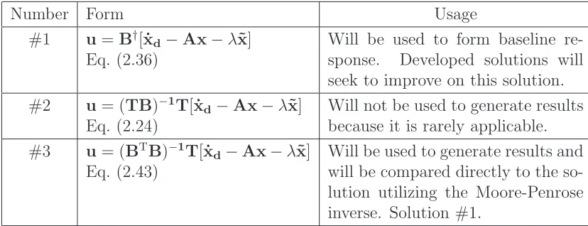
Number Form Usage #1 u=B†[x˙d−Ax−λ˜x]

Eq. (2.36)

Will be used to form baseline re-sponse. Developed solutions will seek to improve on this solution. #2 u= (TB)−1_T_[_x_˙

d−Ax−λ˜x] Eq. (2.24)

Will not be used to generate results because it is rarely applicable. #3 u= (BTB)−1_T_[_x_˙

d−Ax−λ˜x] Eq. (2.43)

[image:43.612.106.520.71.230.2]

Will be used to generate results and will be compared directly to the so-lution utilizing the Moore-Penrose inverse. Solution #1.

Table 2.1: Solution Summary

˙

y−TB(T∗B)−1y˙d+TB(T∗B)−1λ˜y−[TAx−TB(T∗B)−1TAx] =0 (2.46)

does not result in closed loop system dynamics similar to those observed in Eq. (2.9). By not being able to properly form the sliding surface it is not possible to guarantee favorable tracking.

2.7.5

Summary

Overall three solutions have been produced. One solution is based on the established Moore-Penrose pseudoinverse and the other two are based on a pseudoinverse related to the solution of the LQR problem. All three solutions are summarized in Table 2.1.

Solution one will be used to form the baseline results. Solution three will be used because of its ability to match exactly the solution of the LQR problem (for the unforced system). Solution two will not be used because of its inability to match the LQR solution.

2.8

Tracking Performance

Preface

(44)

loop system dynamics. The closed loop dynamics associated with individual states is investigated to determine their ability to track a reference signal.

2.8.1

Dynamic Analysis

In order to evaluate the tracking characteristics of the states the closed loop dynamics between the state vector,x, and the transformed vector,ywill be evaluated. The original system is of the form

˙

x=Ax+Bu

where A represents the dynamic relationship between x and x˙. If the Moore-Penrose pseudoinverse solution is applied to the original system the closed loop system dynamics are developed as follows:

˙

x=Ax+BB†[x˙d−Ax−λx˜]

˙

x=Ax+BB†x˙d−BB†Ax−λBB†x−λBB†xd

˙

x= [A−BB†A−λBB†]

| {z }

Acl

x+ [λBB† BB†]

"

xd

˙

xd

#

where Acl is the closed loop system dynamic matrix. Applying the transform y = Tx

the dynamic relationship becomes

˙

y=TA_clx

The sliding surface is formed for y and y contains the dynamics of each state. Those states with faster dynamics (defined byTAcl) will track more favorably. Or, the primary

components of ywill track better then the less substantial components.

The methodology is similar to the idea of model reduction. Consider the expression

˙

y = [α β] "

x1

x2

#

(2.47)

meaning y˙ is influenced by two states, x1 and x2. Assuming β = 0, Eq. (2.47) becomes

˙

y=αx1

and the solution to this differential equation is

(45)

if α is a large negative number there are few dynamics associated withx1 and in turn y,

meaning favorable tracking.

Now assuming α= 0, Eq. (2.47) becomes

˙

y=βx2

and the solution to this differential equation is

y=x(t = 0)2eβt

if β is a small negative number there are strong dynamics associated with x2 and in

turn y, meaning unfavorable tracking. The conclusion is the larger negative the state coefficient, the more favorable the tracking.

The closed loop system dynamic matrix in y coordinates will be examined as part of the results to determine if the control law promotes favorable tracking of the selected state.

2.9

Linearization and Model Replacement

Preface

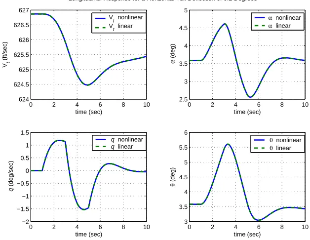
In order to use a linearized model in place of its nonlinear counterpart it must be de-termined if the linear model is valid over the proposed operating region. The nonlinear, longitudinal mode of an aircraft is simulated for various inputs. The linear and nonlinear system responses are observed to determine if the linear model is a valid replacement.

2.9.1

Linearization

Consider the general nonlinear system

y =f(z, t) (2.48)

(46)

operating point ¯z

f(z, t) =f(¯z, t) +

∂f ∂z

T

z=¯z

(z−¯z) + 1

2(z−¯z)

T

∂2_f ∂z2

z=¯z

(z−¯z) +h

Where h represents higher order terms. The first two terms in the expansion constitute a linear approximation of the nonlinear function f(z, t).

Once a linearized version of the nonlinear system is realized it must be validated. More specifically, it must be determined for what region the linearization is considered valid. Since a nonlinear model is linearized about an operating point the model will be exact for that operating point and will be acceptable for some region around that operating point. If the original model is highly nonlinear the system response may diverge severely from its linear counterpart for only small perturbations of z. On the other hand, if the original model does not contain any highly nonlinear terms, the linear and nonlinear system responses may be almost indistinguishable for a relatively larg region about the operating point.

Of course, what is considered “acceptable” must be determined by the engineer. De-pending on the particular application one may be able to tolerate more model divergence. Being able to make this determination is something that comes only with experience.

The nonlinear flight dynamic equations requiring linearization are presented [23]. The Force Equations are

m( ˙u−vr+wq) = −mgsinθ+FAx +FTx

m( ˙v−ur+wp) = mgsinφcosθ+FAy +FTy

m( ˙w−uq+vp) = mgcosφcosθ+FAz +FTz

The Moment Equations are

˙

pIxx−qI˙ xy−rI˙ xz = qr(Iyy −Izz) + (q2−r2)Iyz−prIxy +pqIxz+Mex

−pI˙ xy + ˙qIyy −rI˙ yz = pr(Izz−Ixx) + (r2−p2)Ixz −pqIyz+qrIxy+Mey

(47)

The Kinematic Equations are

˙

φ = p+qsinφtanθ+rcosφtanθ

˙

θ = qcosφ−rsinφ

˙

ψ = (qsinφ+rcosφ) secθ

where m is aircraft mass; p, q and r are aircraft body roll rate, pitch rate and yaw rate, respectively;FAx,FAy and FAz are aerodynamic forces along the aircraft body-axis; FTx,

FTy andTAz are thrust forces along the aircraft body-axis;Mex,Mey andMez are external

applied moments about the aircraft body-axis (mostly aerodynamic but also may include thrust effects); and φ, θ and ψ are the Euler angles, i.e., bank angle, pitch angle and heading angle, respectively. The Force Equations in the stability axis

˙

α = q−(pcosα+rsinα)tanβ− LOM

VT cosβ

+ g

VT cosβ

(cosθcosφcosα+ sinθsinα)

˙

β = psinα−rcosα+ 1

VT

(Y OMcosβ+DOMsinβ)

+ g

VT

(cosθsinφcosβ+ sinθsinβcosα−cosθcosφsinβsinα)

˙

VT = Y OMsinβ−DOMcosβ

g[(cosθcosφsinα−sinθcosα) cosβ+ cosθsinφsinβ]

where

DOM = D−T cosα

m , Y OM =

Y

m, LOM =

L+T sinα

m

The preceding equations are used to simulate the fully nonlinear aircraft response. These same equations are numerically linearized to generate the linear response.

2.9.2

Linear Model Validation and Replacement

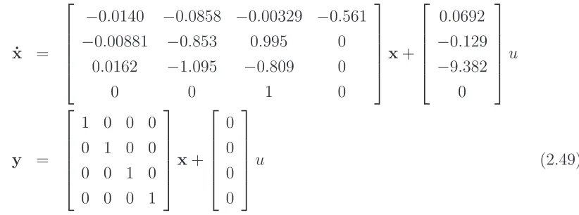
The control architecture being developed as part of this thesis will be applied to a lin-earized, longitudinal model of a high performance aircraft. The state-space form of the longitudinal aircraft model is shown in Eq. (2.49). The state vectorx is defined as

(48)

0 2 4 6 8 10 625.6 625.8 626 626.2 626.4 626.6 626.8 627 time (sec) Vt (ft/sec)

V_t nonlinear V_t linear

0 2 4 6 8 10

3 3.5 4 time (sec) α (deg)

α nonlinear

α linear

0 2 4 6 8 10

−0.8 −0.6 −0.4 −0.2 0 0.2 0.4 0.6 time (sec) q (deg/sec)

q nonlinear q linear

Longitudinal Response for a Horizontal Tail Deflection of 0.1 Degrees

0 2 4 6 8 10

3 3.5 4 4.5 5 time (sec) θ (deg)

θ nonlinear

[image:48.612.159.471.84.323.2]

θ linear

Figure 2.4: Longitudinal linear verses nonlinear aircraft response for for a horizontal tail deflection of 0.1 degrees. State trajectories are nearly identical.

where Vt is true velocity, α is angle of attack, q is pitch rate and θ is pitch angle. The

single input, u, is horizontal tail deflection.

˙ x =      

−0.0140 −0.0858 −0.00329 −0.561

−0.00881 −0.853 0.995 0 0.0162 −1.095 −0.809 0

0 0 1 0

      x+      

0.0692

−0.129

−9.382 0       u y =      

1 0 0 0 0 1 0 0 0 0 1 0 0 0 0 1

      x+       0 0 0 0       u (2.49)

In order to determine whether or not it is acceptable to replace the nonlinear longi-tudinal model with the linearized longilongi-tudinal model, time history response curves are examined. Various horizontal tail deflections are used as inputs and nonlinear verses linear responses are evaluated. Trim condition for the aircraft is straight and level flight at an altitude of 15000 ft. and a velocity of 627 ft/sec.

[image:48.612.127.538.430.583.2]

(49)

0 2 4 6 8 10 624 624.5 625 625.5 626 626.5 627 time (sec) Vt (ft/sec)

0 2 4 6 8 10

2.5 3 3.5 4 4.5 5 time (sec) α (deg)

α nonlinear

α linear

0 2 4 6 8 10

−2 −1.5 −1 −0.5 0 0.5 1 1.5 time (sec) q (deg/sec)

0 2 4 6 8 10

3 3.5 4 4.5 5 5.5 6 time (sec) θ (deg)

θ nonlinear

[image:49.612.158.472.81.324.2]

θ linear

Figure 2.5: Longitudinal linear verses nonlinear aircraft response for a horizontal tail deflection of 0.2 degrees. State trajectories are nearly identical.

does a satisfactory job of approximating the nonlinear response.

Figure 2.5 compares the nonlinear verses linear time history responses of the longi-tudinal states for a horizontal tail deflection of 0.2 degrees. Again, the linearized model does a satisfactory job of approximating the nonlinear response.

Figure 2.6 compares the nonlinear verses linear time history responses of the longitudi-nal states for a horizontal tail deflection of 0.3 degrees. For a deflection of this magnitude divergence becomes evident, most notably of the true velocity and pitch angle. However, this amount of divergence is of no major concern.

Figure 2.7 compares the nonlinear verses linear time history responses of the lon-gitudinal states for a horizontal tail deflection of 0.4 degrees. For a deflection of this magnitude divergence is evident in all states.

Figure 2.8 compares the nonlinear verses linear time history responses of the longi-tudinal states for a horizontal tail deflection of 0.5 degrees. Again, a deflection of this magnitude results in divergence of all state trajectories.

(50)

0 2 4 6 8 10 623 624 625 626 627 time (sec) Vt (ft/sec) V t nonlinear V_t linear

0 2 4 6 8 10

2 2.5 3 3.5 4 4.5 5 5.5 time (sec) α (deg)

α nonlinear

α linear

0 2 4 6 8 10

−3 −2 −1 0 1 2 time (sec) q (deg/sec)

0 2 4 6 8 10

2 3 4 5 6 7 time (sec) θ (deg)

θ nonlinear

[image:50.612.163.471.93.337.2]

θ linear

Figure 2.6: Longitudinal linear verses nonlinear aircraft response for a horizontal tail deflection of 0.3 degrees. Notice mild divergence.

0 2 4 6 8 10

618 620 622 624 626 628 time (sec) Vt (ft/sec)

0 2 4 6 8 10

1 2 3 4 5 6 time (sec) α (deg)

α nonlinear

α linear

0 2 4 6 8 10

−4 −3 −2 −1 0 1 2 3 time (sec) q (deg/sec)

0 2 4 6 8 10

2 3 4 5 6 7 8 time (sec) θ (deg)

θ nonlinear

θ linear

[image:50.612.159.472.420.670.2]

(51)

0 2 4 6 8 10 610

615 620 625 630

time (sec) Vt

(ft/sec)

0 2 4 6 8 10

1 2 3 4 5 6 7

time (sec)

α

(deg)

α nonlinear

α linear

0 2 4 6 8 10

−4 −2 0 2 4

time (sec)

q

(deg/sec)

0 2 4 6 8 10

2 4 6 8 10

time (sec)

θ

(deg)

θ nonlinear

[image:51.612.163.471.263.502.2]

θ linear

(52)

Chapter 3

Results

3.1

Two Mass, Two Spring, Two Damper System

Preface

The first system under investigation is the classical two mass, two spring, two damper model. The system will first be controlled by the control law in Eq. (2.36) and then by the control law in Eq. (2.43) for various Q & R matrices. The closed loop system will be analyzed to validate the effectiveness of the contr