Supervised Material Classification in Oblique Aerial Imagery Using Gabor Filter Features

(1)

Rochester Institute of Technology

RIT Scholar Works

Theses

Thesis/Dissertation Collections

10-5-2014

Supervised Material Classification in Oblique

Aerial Imagery Using Gabor Filter Features

Michael L. Harris

Follow this and additional works at:

http://scholarworks.rit.edu/theses

This Thesis is brought to you for free and open access by the Thesis/Dissertation Collections at RIT Scholar Works. It has been accepted for inclusion in Theses by an authorized administrator of RIT Scholar Works. For more information, please contactritscholarworks@rit.edu.

Recommended Citation

(2)

Supervised Material Classification in Oblique Aerial Imagery Using

Gabor Filter Features

by

Michael L Harris

B.S. Rochester Institute of Technology 2008

A thesis submitted in partial fulfillment of the

requirements for the degree of Master of Science

in the Chester F. Carlson Center for Imaging Science

Rochester Institute of Technology

October 5th 2014

Signature of the Author

Accepted by

(3)

CHESTER F. CARLSON CENTER FOR IMAGING SCIENCE

COLLEGE OF SCIENCE

ROCHESTER INSTITUTE OF TECHNOLOGY

ROCHESTER, NEW YORK

CERTIFICATE OF APPROVAL

M.S. DEGREE THESIS

The M.S. Degree Thesis of Michael L Harris has been examined and approved by the

thesis committee as satisfactory for the thesis required for the

M.S. degree in Imaging Science

David Messinger Ph.D, Thesis Advisor

Harvey Rhody Ph.D

Carl Salvaggio Ph.D

Date

(4)

Supervised Material Classification in Oblique Aerial Imagery Using

Gabor Filter Features

by

Michael L Harris

Submitted to the

Chester F. Carlson Center for Imaging Science in partial fulfillment of the requirements

for the Master of Science Degree at the Rochester Institute of Technology

Abstract

RIT’s Digital Imaging and Remote Sensing Image Generation (DIRSIG) tool allows modeling of real world scenes to create synthetic imagery for sensor design and analysis,

trade studies, algorithm validation, and training image analysts. To increase model

con-struction speed, and the diversity and size of synthetic scenes which can be generated it is desirable to automatically segment real world imagery into different material types and

import a material classmap into DIRSIG. This work contributes a methodology based on

standard texture recognition techniques to supervised classification of material types in oblique aerial imagery. Oblique imagery provides many challenges for texture recognition

due to illumination changes with view angle, projective distortions, occlusions and self

shadowing. It is shown that features derived from a set of rotationally invariant bandpass filters fused with color channel information can provide supervised classification accuracies

up to 70% with minimal training data.

(5)

Acknowledgements

This work would not be possible without the support and insight of my advisor Dr. David

Messinger and the RIT Digital Imaging and Remote Sensing Lab and staff. I would also like

to acknowledge my committee members for their guidance and instruction. Finally, I am incredibly appreciative of my officemates who, amid laughter and shenanigans, provided

an enjoyable and stimulating working environment.

(6)

Chapter 1

Introduction

Because of the expensive nature of performing field campaigns and testing imaging sensors

in real world conditions, simulation of their design and operation is often performed in

virtually rendered environments. Within these environments, an incident spectrum, atmo-spheric parameters, object geometry, and material properties are loaded, and an internal

physics based engine calculates the path of radiation propagation to finally model the

sensor reaching radiance. This allows simulation of final image quality of an arbitrarily complex scene, and is an aid to developing sensor specifications, classification algorithms

and the like.

To generate synthetic scenes, it is necessary to manually develop the 3D object geom-etry, and hand label all of the material types on each facet. This is very time consuming

and prohibits the fast generation of larger scenes, and therefore the diversity that can be

simulated within a scene. It also makes it difficult to generate synthetic imagery of real world scenes for simulation, since each object needs to be manually fabricated identically

to the real world version. Given the constraints that manual model generation imposes,

it is desirable to automate the procedure. This requires the automatic generation of both the geometry, and the material labels of a scene to be rendered. For the purpose of

gen-erating synthetic images of real world scenes this will involve the collection of data over

a particular site of interest, transforming this data into both a geometrical model of the objects therein, and labeling each homogeneous object part with a material type. These

can then be used as inputs to a synthetic image generation (SIG) software to simulate real

world scenes.

Recent advances in computer vision that will be briefly discussed allow geometric

(11)

6 CHAPTER 1. INTRODUCTION

models to be generated from a collection of overlapping images in an automated workflow. In particular, this means that scene geometry can be created from aerial imagery, satisfying

the need for one input in SIG software. The remainder of this work will focus on satisfying

the second SIG input, the classification of the scene to be rendered into various material types. This will be done using the standard methodology of supervised classification.

A feature set based on filter responses will be investigated, as well as the inclusion of

color channel information. The emphasis is on determining how much training data (and therefore user interaction) is required, and whether standard texture features lead to

adequate separability and classification accuracy on a challenging dataset of oblique aerial

imagery taken over the Purdue University campus.

It is the goal of this work to develop and test a classification scheme that produces

a salient class map that can be incorporated into SIG software to aid in automatic

syn-thetic scene generation. The success of the classifier will be based on its overall accuracy, the individual class accuracies, its ability to incorporate diverse training data, and finally

the quantity of training data necessary to produce acceptable results. Such a non-critical

application does not require a high degree of accuracy or speed, but looking toward mini-mizing human intervention, the goal is minimal training data selected, automated

param-eter dparam-etermination (if necessary), and high accuracy. The next sections in this chapter

will briefly overview the operation and requirements of the SIG software at RIT called DIRSIG, the state of RIT’s 3D extraction workflow, as well as detail the challenges of

the aerial imagery used in the classification procedure developed. Finally, previous work

which motivates the use of texture and color features in a supervised classification system will be discussed.

1.1

DIRSIG Scene Generation and Requirements

Modeling radiative transfer mechanisms along with the world’s geometry allows simulation of the sensor-reaching radiance of a fabricated scene. RIT’s Digital Imaging and Remote

Sensing Image Generation (DIRSIG) tool provides an environment to model source

geom-etry, atmospheric propagation, wavelength and geometry dependent spectral characteris-tics, and sensor operation [1]. DIRSIG can be used to complement real ground truth in,

for example, the exploration of target detection or classification algorithm performance,

(12)

[image:12.612.105.526.122.417.2]

1.1. DIRSIG SCENE GENERATION AND REQUIREMENTS 7

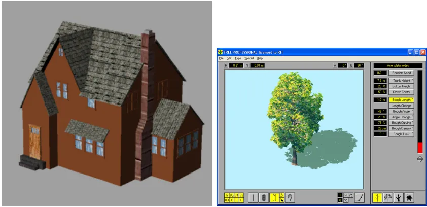
Figure 1.1: DIRSIG Megascene bird’s eye and detail views.

will provide an overview of DIRSIG’s features and look into the user inputs required for

generating synthetic imagery.

In addition to the source geometry, the required model inputs include the Bidirectional Reflectance Distribution Function (BRDF) within each representative material, as well as

a texture map that facilitates spatial variation in the reflectance spectra. The material

library has been generated from extensive ground truth measurements and contains hun-dreds of materials characterized under various conditions. This is used as a lookup table

to induce the spectral character of each facet in the model.

Currently, base models of several types of vehicle, house, tree, industrial building and

the like are fabricated by hand using a variety of Computer Aided Design (CAD) tools, and each material is specified. These base models are then attributed with varying materials

and orientations and instantiated manually throughout the scene. Though scenes on the

(13)

8 CHAPTER 1. INTRODUCTION

dynamically for real world scenes. Automating this procedure would allow fast replication of real-world environments and structures, greatly increasing the diversity, complexity, and

efficacy of simulation. This task requires the automatic generation of two inputs, namely

the source geometry of the scene to be rendered, and a classmap of material type coupled to each facet of the geometry to leverage the DIRSIG material property database. Both

of these inputs can be derived from images of the desired scene to be rendered.

Figure 1.1 shows a portion of a synthetic image constructed and rendered in DIRSIG

that covers several square kilometers. To render this scene several external inputs are required. First the scene geometry must be in place. Figure 1.2 shows objects manually

crafted from in-house and commercial CAD modeling packages. For each object several

base models are created having different geometrical properties. Multiple building types, vehicles, and species of vegetation have been created as base models. To account for

variability in color, texture, orientation, and size the base models are attributed with these additional properties and hand placed over the scene. For example a base model house

may be fabricated then attributed with different roofing or siding types and subjected to

several affine transformations to create a variety of houses in a residential scene. This leads to the ability to simulate diverse environments but is very time consuming and requires

fabrication of a new base model any time a unique structure is simulated.

To employ radiometrically correct physical modeling of light interaction each facet

of every instantiated object is labeled with a material linked to a database of material properties. The strategy for introducing objects with diverse spatial and spectral character

is to draw from a large database of reflectance curves which contain variability induced

by surface inhomogeneities as well as a BRDF model to account for variation in surface orientation. Spectral reflectance curves for a large number of materials have been built

up over multiple large scale field campaigns to support simulation activity. In addition to

reflectance every material has associated thermal properties such as emissivity allowing simulation in the infrared portion of the EM spectrum. Thus every facet requires a material

label in order to leverage this library.

For rendering to accurately model sensor reaching radiance a robust atmospheric model

also needs to be in place to account for scattering and absorption of EM radiation. DIRSIG can work with commonly used MODTRAN atmospheric profiles which specify solar

illu-mination conditions and atmospheric conditions such as aerosol count, water vapor, and

(14)

[image:14.612.102.523.127.331.2]

1.1. DIRSIG SCENE GENERATION AND REQUIREMENTS 9

Figure 1.2: Object models generated by external software packages for inclusion in a DIRSIG simulated environment.

of various noise sources, integration over relevant bands, and spatial resolution on the

output image.

Note that every input has spectrally dependent characteristics, leading to the

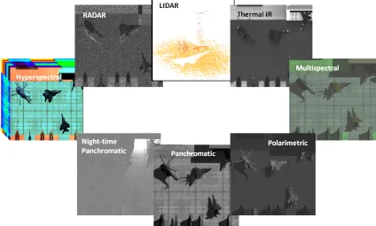
abil-ity to simulate a variety of imaging modalities. Figure 1.3 shows synthetic images of an aircraft generated utilizing visible and infrared bands in multi and hyperspectral

config-urations, as well as thermal and polarimetric bands. This reinforces the concept that for

radiometrically accurate modeling each object facet requires specification of a particular material type and associated properties. The following sections will detail progress toward

automating the construction of DIRSIG scene models particularly the generation of scene

geometry, and material classification.

1.1.1 3D Extraction Workflow/Geometry Input

Toward automating construction of 3D models RIT has developed a workflow to automate

point cloud extraction from a series of images based on point correspondences and pho-togrammetric principles [2]. Recently, the maturation of this work has allowed production

of geo-located structural models [3]. These algorithms make it possible to capture aerial

(15)

[image:15.612.151.575.266.521.2]

struc-10 CHAPTER 1. INTRODUCTION

(16)

1.1. DIRSIG SCENE GENERATION AND REQUIREMENTS 11

(a)

[image:16.612.100.528.128.332.2]

(b)

Figure 1.4: 3D extraction workflow description (1.4a) and illustration (1.4b)

tural model useful for simulation or other tasks such as urban development or mission

planning where knowledge of 3D scene geometry is critical. This represents a leap forward in automatic generation of source geometry for simulation.

Figure 1.4 shows a snapshot of the 3D extraction workflow and several facetized build-ing models. As is evident the buildbuild-ing sides do not contain much detail; this is due to the

use of only nadir looking imagery. Research is ongoing to overcome the challenges

associ-ated with using oblique captures. Such challenges include finding correspondences among points which have undergone large rotations and perspective distortions and dealing with

occlusions.

It is important to note how the availability of facetized models impacts the material

classification procedure that is to be developed in the remainder of this work. The 3D

extraction process results in images that are co-registered with a 3D model. In order to label a material type for each facet, some segmentation of the image must be donea priori

that extracts the interesting components such as buildings at the object level. This allows

the classifier to work on homogeneous regions such as rooftops and building fa¸cades rather than on the entire image. The work required to segment 3D models and label rooftops

and fa¸cades is ongoing, and will be assumed to be possible for the purpose of this work.

(17)

12 CHAPTER 1. INTRODUCTION

be done using the 3D data.

1.1.2 Material Label Input

The remainder of this work will address the second criteria of automated model generation

for simulation: extraction of material type from images of the scene to be rendered. As discussed above this will be formulated as a supervised classification problem with the

user identifying training regions in an input image of interesting material classes, and the

classifier labeling all other regions in that and remaining images with a material type. As above, it is assumed that the sample images are already segmented into rooftops, building

fa¸cades, and other object components (in this work this will be done manually). Next,

the test dataset details are presented, and these and previous work will be used to select specifics of the classifier.

1.2

Data

The previous section laid out the problem of classifying material type from aerial imagery.

This section will detail the specifics of the dataset that is available to test the procedure.

1.2.1 Specifics of this problem with oblique aerial imagery

Section 1.1 reviewed the input requirements for simulation of the image formation process

of a modeled scene. These included both model geometry, and material labels for every facet of the model to render spatial/spectral interaction properties. In order to acquire

accurate and geometrically detailed models, oblique views of the input structures are

re-quired. This also facilitates classification of building rooftops and facades. Aerial imagery with cameras poised at oblique angles provides a fast and reliable way of obtaining detailed

imagery of large areas. Particularly interesting areas for simulation include urban and

res-idential environments. As noted in the above considerations there are several challenges to classifying oblique aerial imagery of densely populated areas. These include the projective

distortions associated with oblique look angles, varying solar illumination, varying object

(18)

1.2. DATA 13

Details of the data

The goal in acquiring a dataset was to develop and demonstrate a feature extraction and

classification mechanism to identify the material type from oblique imagery of urban areas. A material classmap would then be combined with the geometry derived from the 3D

extraction process of Section 1.1.1 which is being developed in tandem by other researchers

at RIT. Data that was readily available included high resolution oblique imagery of the Purdue University campus from Pictometry Inc. Pictometry provides imagery of 4 look

angles (pointed ahead, behind, right, and left of flightpath) and an orthorectified nadir

shot. Only the standard RGB bands are available, and the resolution is about 1₂ ft per pixel dependent on flying altitude.

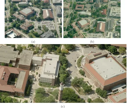
Three collects of this area were performed, each at increasing resolution down to 2

inches, shown in Figure 1.5. At the coarsest resolution only the aggregated effects of tex-ture are visible rather than individual shingles or brick and mortar. Higher resolutions

offer richer textural content and may provide guidelines for the imaging conditions

neces-sary to accurately label materials on oblique objects using only 3 bands. The following are details of the challenges of classification of oblique aerial imagery.

Projective Transformations

In purely nadir looking capture conditions all objects in the image lie approximately in

the ground plane and transformations include primarily similarities (rotations and

trans-lations). For a single image the sensor elevation is also approximately constant so the scale at which objects and textures present themselves is constant. These transformations

preserve angles and edge lengths so the underlying structure of any visible texture will

remain the same. This is not the case in oblique imagery, where projective distortions vary this underlying structure such that a periodic rectangular array such as a brick wall will

no longer appear rectangular, and additionally will be periodic with a different frequency.

Projective distortions also change the scale at which a texture feature occurs

through-out the image. All image objects and textures are no longer an equal distance from the sensor, so the resolution varies pixel to pixel. Effectively this means that the same texture

is sampled at different rates in different parts of the image, and will change in appearance

(19)

14 CHAPTER 1. INTRODUCTION

(a) (b)

[image:19.612.156.578.219.579.2]

(c)

(20)

1.3. PREVIOUS WORK 15

Illumination

Depending on the sun-sensor angle an image will exhibit variations in specularities,

shad-owing, and occlusions. These will affect both the pixel intensity and spectral character. Noise may also dominate in areas of low light, changing the appearance of texture. The

spectrum of solar illumination will also vary with changing atmospheric conditions and

date. This will have an effect on the reflected spectra of objects in the scene and will especially make use of spectral content difficult.

Clutter

A challenge to geometry extraction as well as material identification is the presence of occlusions and clutter in the scene. Clutter will be defined as any part of the image that is

irrelevant to the classification mechanism and can possibly introduce error. A prominent

source of clutter in urban scenes are windows. Any feature generation mechanism that operates over a region will pick up window pixels along with the building pixels that

are interesting to the classifier, and essentially add a nonuniform source of noise. Other

sources of clutter and occlusion include cars and other objects on rooftops that both add noise and obscure the underlying interesting regions.

1.3

Previous Work

After having a look at the dataset that is available and its challenges, we next consider

related work that has been done to advance the field of scene classification. Both of these will inform the selection of an appropriate classifier, and its details will be developed.

1.3.1 Classification Task

Before looking at previous work, the details of the classification task will briefly be pre-sented as they are relevant to the choice of classifier. The classification task can be

divided into two subtasks, the first of which is selecting features of the data that allow

for separability of unique classes in the dataset. It is not necessary for these features to completely describe the data, only to represent the data in such a way as to promote class

discrimination. For example a pixel’s value in the green channel taken as a feature from

(21)

16 CHAPTER 1. INTRODUCTION

but would not be adequate for distinguishing between types of vegetation. There are many texture and color features that are often used, and it is important to select those that best

fit for the given dataset.

The second task is the labeling of regions in the image. This work will only consider the case of supervised classification rather than clustering because we wish to label regions with

a certain class value rather than agnostically group the data according to mutual similarity.

This task uses input training examples to model the appearance of a representative class in feature space and then labels regions with a class value according to a similarity criterion.

Both of these tasks have been well studied and there is a wealth of related work dealing

with optimal feature generation, and advanced classification algorithms. The following will detail related work in the area of feature selection, and classification.

Feature Generation Task

The first task of a classifier is to represent an image in terms of features that lead to

optimal separation of the constituent classes in feature space. Because in this work we are dealing with three band RGB imagery it seems likely that textural metrics will provide

necessary features in addition to the color channel intensities. For the purpose of material

identification, textural metrics seem necessary in addition to color information due to aesthetic variations in materials such as brick, siding, and residential roofing. Therefore

we are also interested in determining the extent to which color and texture features can

or should be combined to enhance classification.

Previous work in texture analysis for the purpose of classification has focused on four

main texture metrics, these being statistically derived (such as moments), model based,

structural and geometrical, and finally filter based [4]. No single feature set has been discovered which should be used in every case, rather constraints on computational

com-plexity, ease of implementation, and efficacy for a given dataset should guide the choice of

feature set. Much recent work has been dedicated to the understanding and advancement of filter based methods [5, 6, 7, 8, 9] and excellent classification results have been achieved

on a wide variety of texture databases, natural imagery, and moderate resolution satellite

imagery. The major advantage of filter based approaches is they are inherently multires-olutional [10]. Traditional methods such as gray level co-occurrence features [11] analyze

moments over the entire image spectrum, whereas a multiresolution approach is able to

(22)

1.3. PREVIOUS WORK 17

This leads to the potential for increased discrimination of textures of varying frequency content. The review paper of Randen [6] concludes extensive tests with the result that,

although there is no clear winning feature extraction technique for every case, filter based

methods typically outperform the traditional methods. In addition, the GLCM method is more computationally demanding than filter based methods. As pointed out in [5] the

Gabor filter implementation in [6] could have been improved with better filter spacing.

Each of the above philosophies of feature extraction focuses on representing texture

in various ways, and pulls out features that should be indicative of different textured regions. The mean, variance, and other higher order moments are examples of statistical

descriptors that attempt to quantify and discriminate between texture regions. The filter

based approaches produce features based on the response of a given texture region to a bank of filters, and can be quickly applied in the frequency domain. It is not the purpose

of this work to develop a novel feature generation technique, but rather to investigate the

application of standard techniques to an interesting dataset. Therefore, because of the fundamental underpinning of the filter based methods in frequency analysis, we will focus

on these methods.

Classification Task

Once salient features have been identified and extracted the supervised classifier’s task is to group the data according to similarity to the training samples. Most classifiers can be

thought of as methodologies of constructing decision boundaries around the training data,

such that a point in feature space which falls within a given boundary, is labeled a member of that particular class. Concerns similar to selecting a feature set exist in selection of

a classifier, such as computational intensity, and whether the decision boundary shapes

(hypersphere, hyperellipsoidal) fit the data.

1.3.2 Classification Based On Texture

Because the data available is three band imagery, the color content alone may not be

enough to ensure good classification. Therefore we first look at previous work involving

(23)

18 CHAPTER 1. INTRODUCTION

Gabor Filters

Because of similarity to the human visual system [12], the Gabor filter has garnered much

attention for texture analysis [13, 14] in the areas of segmentation [10, 5], content-based

image retrieval [15, 7], as well as supervised classification [16, 17], and facial recognition [18]. Typically, texture databases have been used to test various configurations of a Gabor

filter bank on classification accuracy. In cases where remotely sensed data were used, the

resolutions have been moderate, and the textures have consisted primarily of nadir looking satellite images of broad regions of built-up, forested, or water.

The Gabor filter has been favored over other filters [6] due to its optimal localization in

the spatial and spatial frequency domains [19], and its flexibility to be arbitrarily specified

in many configurations. It can be easily specified at any spatial frequency center frequency, orientation, and with any bandwidth. This makes it suitable as a bandpass filter for

extracting dominant frequencies in textured images. It is also mostly insensitive to global

variations in intensity, which is a necessary feature in classification of real scenes.

Good results have been achieved in supervised classification of satellite imagery [16, 17], however there have been no studies using this filter based approach on higher resolution

aerial imagery for the purpose of material identification. Because of the promising previous

results, and desirable properties, the Gabor filtering scheme will be tested on the novel dataset described above.

Invariant Texture Features

The nature of the test dataset ideally requires some invariance to affine distortions,

ro-tations, and illumination variation, described in Section 1.2.1. Features based on texture rather than spectral character immediately provide some robustness to changing

illumina-tion levels, though less to changing illuminaillumina-tion direcillumina-tions. Previous work also provides a

simple way of providing some rotation invariance to the Gabor filtering scheme, which will be described in a later chapter. The Gabor filter’s spatial extent and flexible control over

its bandwidth should also provide some degree of invariance to other affine distortions,

(24)

1.3. PREVIOUS WORK 19

Classification

Once a feature set has been generated, in this case using texture features, the remaining

task is to label image regions according to similarity to training data. The simplest way of doing this is with a minimum distance classifier, which assigns each region a class label

based on its direct proximity in feature space. In this work we are mainly concerned with the efficacy of the feature set, so the simplest approach will be used. The Bhattacharyya

distance is commonly used to compute separation between two distributions in feature

space [20], and will be used here to measure distances between distributions taken from test image regions, and each training distribution. To measure distances from an individual

feature vector to a training distribution the Mahalanobis distance will be used [20]. Both of

these distances are normalized by the covariance of the training (and the test distribution in the former case) data and assume hyperellipsoidal class boundaries, which are suitable

for use with Gabor filters [5]. Because both of the previous distances assume normal

data, another minimum distance method will be computed by packaging the data as a histogram. This method avoids covariance estimations, and statistical assumptions, and

is easy to apply as well.

1.3.3 Combining Color and Texture

Although the color channel information may prove to be erroneous due to the changing

illumination conditions over multiple images, we will examine several ways of doing so and their impact on the resulting classification accuracy.

Color Spaces

The standard RGB image representation is highly correlated from band to band, so for

this work we will use the alternativeL∗a∗b∗ color space described in [21]. This color space

has the advantage that its bands are approximately orthogonal, and additionally, split the spectrum into an overall illumination or intensity component, and two chromaticity

components. Thus, for texture analysis, the intensity channel can be filtered, and the

(25)

20 CHAPTER 1. INTRODUCTION

Color Texture Fusion

Previous work has shown several methods of combining color and texture information

[22, 23, 24, 25]. In [22] Gabor filtering of each color channel was proven a successful method of extracting color-texture features. The major lines of research have investigated

joint and separate color-texture processing. One na¨ıve method, and two other simple methods which have shown promise will be investigated.

The first is to first generate texture features, then simply concatenate the color channel

intensities onto each texture feature vector. The next is to filter every color channel, generating a texture feature vector for each channel, and concatenating those, as in [23].

The last is to classify using only the texture features, and again using only the color channel

intensities, then combine the outputs of the two classifiers to generate the final classmap. Work on multiple classifier fusion such as [26] provides very simple voting methods that

will be used here.

1.3.4 Conclusion

The problem of classifying oblique aerial imagery for the purpose of synthetic image

gen-eration has been presented along with the challenges of this particular dataset. The

methodology for classification takes advantage of the fact that the 3D processing leads to a geometric model that is co-registered with the images, such that whole buildings,

as well as their rooftops, facades, and other components can be segmented out of the

images, leaving ideally homogeneous textured regions. Because of the deficiency in color information, the texture information should provide additional discriminatory power for

producing a thematic map of material classes. Although there are many textural metrics

that have been generated, because of flexibility, widespread use, ease of implementation in the frequency domain, robustness to affine and illumination variations, and proven success

in many areas, the Gabor filtering scheme will be used to extract textural information.

Several methods of fusing color channel information will also be used.

The main goal of the following sections is to determine the efficacy of commonly used

textural features in classifying a dataset which presents novel challenges, as well as the

extent to which color channel information can or should be used in the task. Because the dataset includes three different resolutions, the results assessment should give some

guidance as to the resolution required to adequately capture textural information with

(26)

1.3. PREVIOUS WORK 21

classification task - should test regions first be segmented and the textural features ag-gregated before classification, or should each pixel be classified and then the classmap

(27)

(28)

Chapter 2

Methodology

2.1

Filtering for Texture Analysis

This section will detail the application of a filter bank for texture analysis, the type of

filters used and their suitability for this application, the nature of the derived feature sets,

and the classification algorithm used.

2.1.1 Overview of Filtering Scheme

The filtering approach to texture analysis is grounded in the fact that textured images can be represented by their frequency content, or lack thereof, and by designing a filter which

responds to the appropriate frequencies, textural metrics can be extracted. These metrics

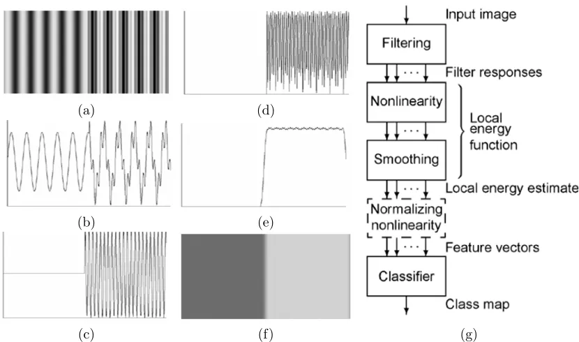
can then be used for concise texture representation, image reconstruction, and discrimi-nation among various textures [16, 5, 27]. Figure 2.1 details a schematic of this process

in the context of classification of textured images. First an input texture image, assumed

to be homogeneous, and contain one or more dominant frequencies, is convolved with a filter tuned to one of those dominant frequencies. Next, a feature is generated by taking

some non-linearity, such as an energy function, and smoothing is performed. Therefore a

textured image is represented by the energy contained in its dominant frequency band.

Two or more textures can be segmented by estimating their dominant frequencies, and constructing one or more filters (equal to one less than the number of textures) tuned to

these dominant components. In the case of many textures, or where it is inefficient to first

estimate all of the dominant components, a filter bank which covers the entirety of the

(29)

24 CHAPTER 2. METHODOLOGY

(a) (d)

(b) (e)

[image:29.612.153.568.128.373.2]

(c) (f) (g)

Figure 2.1: Process of applying a single filter to an input texture image of two dominant frequencies (a). An amplitude profile of the image (b). Result of applying filter tuned to the texture in the right half of input image (c). Rectification (or other non linearity) (d), and finally smoothing (e). The output amplitude contrasts the two different textures (f). The process in algorithmic form (g). Graphic included from [6]

frequency spectrum can be designed [10]. In this case each texture is then represented by

a feature vector of responses to each filter, and classification is performed. The particular

filter choice and placement in the frequency domain depends on the location of relevant frequencies in the image, and will be discussed below.

2.1.2 Gabor Filter

Gabor Wavelet

The methodology of decomposing a signal into its dominant frequency components has

been well studied in signal and image processing. One special criteria for local texture recognition is localization of the filter in both space and spatial frequency. It has been

shown that the (complex) Gabor filter satisfies this criteria in the sense that it minimizes

(30)

2.1. FILTERING FOR TEXTURE ANALYSIS 25

isolates spatial frequency content in a localized portion of the image1.

The 2D Gabor wavelet is a Gaussian function modulated by a complex sinusoid as in

g(x, y) =s(x, y)wr(x, y) (2.1)

where the complex sinusoid is denoted bys(x, y), the Gaussian envelope bywr(x, y), both

with 2D spatial coordinates (x,y). The sinusoid has the effect of specifying the center frequency and orientation of the filter. This produces a spatial frequency bandpass filter

that can be arbitrarily located and oriented.

The complex sinusoid is given by

s(x, y) = exp(j(2π(u0x+v0y) + Φ)) (2.2)

with frequency locationu0andv0, and initial phase Φ. In polar coordinates the magnitude

F0 and directionω0 are respectively

F0 =

√

u0+v0, ω0= tan(

u0

v0

) (2.3)

and the equation becomes

s(x, y) = exp(j(2πF0(xcosω0+ysinω0) + Φ)). (2.4)

The real and imaginary components of the complex sinusoid (Figure 2.2) are respectively

Re(s(x, y)) = cos(j(2π(u0x+v0y) + Φ)) (2.5)

Im(s(x, y)) = sin(j(2π(u0x+v0y) + Φ)). (2.6)

The Gaussian envelope (Figure 2.2) is specified as

wr(x, y) =Kexp(−π(a2(x−x0)2r+b2(y−y0)2r)) (2.7)

1

(31)

26 CHAPTER 2. METHODOLOGY

(a) (b) (c)

(d) (e) (f)

Figure 2.2: Real (2.2a) and imaginary (2.2b) parts of the complex sinusoid component of a single Gabor function. Real (2.2c) and imaginary (2.2d) parts of the Gabor function. Gaussian component (2.2e), and frequency domain showing 4 Gabors (2.2f) from 0 to 135 degree orientations.

with subscriptr indicating a rotated coordinate system given by

(x−x0)r= (x−x0) cosθ+ (y−y0) sinθ (2.8)

(y−y0)r=−(x−x0) sinθ+ (y−y0) cosθ, (2.9)

and a and b give the extent of the ellipse along the major and minor axes. This

windowing function produces the desirable spatial/spatial frequency localization properties

of the Gabor function. It is also apparent that the real and imaginary components of the function are nearly equivalent but for a 90 degree shift in phase, so they approximately

form2 a quadrature pair. The analytic portion of any filtered signal can then be extracted by discarding the phase.

2_{The cosine component contains some DC response which must be eliminated to produce an actual}

(32)

2.1. FILTERING FOR TEXTURE ANALYSIS 27

Properties

We will now investigate the specification of the above parameters and their relation to

the multichannel filtering approach to texture recognition. The Gabor function in polar coordinates is

g(x, y) =

Kexp(−π(a2(x−x0)2r+b2(y−y0)2r))

exp(j(2πF0(xcosω0+ysinω0) + Φ)). (2.10)

This can be rewritten in terms of a standard deviation σ and aspect ratio λas

g(x, y) = 1

2πλσ2exp(−

(_λ12(x−x0)2r+ (y−y0)2r)

2σ2 )

exp(j(2πF0(xcosω0+ysinω0) + Φ)). (2.11)

where, for normalization to a maximum of unit magnitude in the frequency domain, we

requireK = ₂_πλσ1 2 =ab.

In the frequency domain, the Fourier transform of the Gabor function gives

G(u, v) =

exp(−2π2σ2(λ2(u−u0)2r+ (v−v0)2r))

exp(j(−2π(x0(u−u0) +y0(v−v0) + Φ))) (2.12)

with magnitude and phase in polar coordinates

Magnitude(G(u,v)) = exp(2π2σ2(λ2(u−u0)2r+ (v−v0)2r)) (2.13)

Phase(G(u,v)) = exp(j(−2π(x0(u−u0) +y0(v−v0) + Φ))). (2.14)

The form of this equation produces an ellipse with center located at (u0, v0) or (F0, ω0),

major axis length proportional to σ and aspect ratio λ. This allows specification of a bandpass filter of arbitrary location and orientation. In general only filters with polar

angle equal to orientation angle are useful since any other configuration will lead to an

(33)

28 CHAPTER 2. METHODOLOGY

Figure 2.3: Specification of the frequency, BF, and orientation, Bθ, bandwidths, and

angular spacingSθ of a Gabor wavelet.

can be derived [29] respectively as

B = log₂(πF λσ+α

πF λσ−α) (2.15)

whereα=plog₂2/2 and

Ω = 2 tan−1(α/πF σ). (2.16)

Figure 2.3 shows the details of these specifications on the frequency spectrum of a Gabor wavelet.

Thus it is possible to construct a bank of filters of varying center frequency and

orien-tation to achieve complete coverage of the frequency domain. A textured image can then

(34)

2.1. FILTERING FOR TEXTURE ANALYSIS 29

a localized image region whose size is dependent on the characteristic lengthσ and aspect ratioλ. This representation can be thought of as a localized expansion of the image using

the Gabor wavelets as an independent set of basis functions. The energy contained in the

coefficients of the expansion are then used as textural features.

Filter Bank Design

Since the frequency content of an image and its constituent classes may not be known a

priori, it may be necessary to incorporate a bank of filters each tuned to a separate portion

of the frequency domain. As above there are many free parameters of the Gabor filter that can be tuned, which can essentially be broken down into the frequency bandwidth,

center frequency, and orientation. Furthermore for a bank of filters, the number of filters

and their angular and frequency spacing is also variable. It is important to specify these parameters to maximize information extraction.

The dyadic configuration in [10] is widely used because it produces nearly uniform and entire coverage of the spatial frequency domain. Figure 2.4 shows examples of this

arrangement. The foundation of this approach is in the assumption that most texture

content is found at lower frequencies, and so the resolution should be higher there for increased discriminatory power. As a consequence of this arrangement, higher frequencies

are sampled with lower resolution.

This leaves the angular spacing, the bandwidth, and the number of filters to be set.

[5] uses an angular spacing of 30◦ , and in [10] the number of filters is set such that the

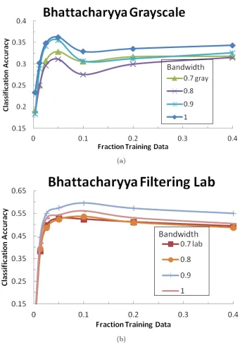
highest frequency filter’s center frequency lies just inside the window of Nyquist aliasing. Since the bandwidth is probably imagery specific, it will be left as a free parameter to be

tuned on each imagery dataset used. Heuristic guidelines for its range appear in [16], to

be between 0.7 and 1.5.

2.1.3 Feature Extraction

Filter Bank Feature Extraction

As shown in Figures 2.1 an input image is convolved with a bank of filters each tuned to a different portion of the frequency domain. The filtered output at this stage is still

oscillatory in the spatial domain, and requires some form of rectification and averaging

(35)

rec-30 CHAPTER 2. METHODOLOGY

Figure 2.4: 32×32 Dyadically spaced Gabor filter bank containing 4 center frequencies and 12 orientations. Each filter center frequency is one octave above the lower one.

tification have been proposed and investigated, and all involve application of a non-linear

function, most often one that computes the energy (complex magnitude) of the filtered response [5]. Others have included taking only the real component of the filtered output,

absolute value, and use of a sigmoidal function.

Since this has been thoroughly investigated we will use the simple approach of

tak-ing the absolute magnitude of the filter responses to derive one feature per pixel of the convolved image, as well as the variance of the area within the filter extent to derive a

second feature. These features were shown to be effective in [5]. Additionally using the

simple absolute magnitude avoids additional parameters in defining a suitable non-linear function.

Following rectification, smoothing can be performed to produce a uniform output. To do this a smoothing function is applied to each rectified filtered output that is the same

shape and orientation as the Gaussian component of the filter used to generate the output,

but with a wider extent [16, 5]. The smoothing parameterγ is used to control the extent of smoothing simply by scaling the coordinate system of the Gaussian component as in

g(x, y)→g(γx, γy). (2.17)

(36)

2.2. CLASSIFICATION 31

Rotation Invariance

Several authors have provided an elegant method for deriving rotationally invariant

fea-tures from the outputs of the filter responses detailed above [30, 31]. This method relies on the fact that along the orientation axis, the filter responses are periodic, and therefore

a rotation of the image simply shifts the response along the rotation axis. As long as there is adequate coverage then the response of an image with textures oriented at 0◦ will

ring the 0◦ oriented filter, and when rotated, will excite an adjacent filter tuned to that

orientation. This means that rotations of the input image are mapped to translations along the orientation axis.

Because of this periodicity and mapping, if a DFT is taken along the orientation axis

for each response, the property of shift invariance will lead to identical DFT coefficients for images undergoing only rotational transformations. Half of the DFT coefficients are

redundant due to even symmetry when operating on real signals but the remaining

coef-ficients are rotation invariant. This procedure can be used to achieve rotation invariance on both the rectified signal outputs, and the variance outputs. Figure 2.5 shows this

procedure by filtering two rotated sinusoids. The rotated spectra fall on different Gabor

wavelets leading to a shift in the overall response along the orientation axis. The response of an individual pixel in the 45◦ sinusoid is seen to shift two indices to the right in the

plot of Gabor coefficients, but the 45◦ and 0◦ sinusoids DFT coefficients line up well.

2.2

Classification

After deriving features which in this work are textural metrics derived from the output of filter responses each region is assigned a class label using a distance metric. In this work

a simple minimum distance classifier is used rather than a more advanced and

computa-tionally expensive one so that the emphasis is on the choice of feature set, rather than the choice of classifier.

2.2.1 Minimum Distance

The minimum distance classifier labels a particular region with the class label of the overall class distribution it is closest to in feature space. Two minimum distance classifiers will

be used to test the efficacy of the derived feature sets, the Bhattacharyya distance, and

(37)

32 CHAPTER 2. METHODOLOGY

(a)

(b) (c)

(38)

2.2. CLASSIFICATION 33

an attempt to estimate the probability distribution function underlying the data without assuming a specific parametric model.

Bhattacharyya Distance

A well known parametric statistical distance is the Bhattacharyya distance which accounts

for the mean and spread of the sample and reference multidimensional distributions [20].

By estimating the mean µand covarianceS, and assuming a Gaussian model as follows

DB=

1

8(m1−m2)

T_S−1₍_m

1−m2) +

1 2ln(

detS √

detS1detS2

), (2.18)

the distance of each test to each reference distribution (subscripts 1 and 2 respectively) is calculated and a class assignment is made. This parametric model relies on the assumption

of normal feature distributions, which is appropriate for Gabor filter features [5]. A major

drawback to this model is the need to estimate accurately the covariance, and compute matrix inverses, which for high dimensional data requires large sample sizes. This may

not be possible for smaller segmented texture regions, and high dimensional feature sets.

χ2 Distance

To bypass the unwieldy covariance terms in the Bhattacharyya distance and relax the

assumption of Gaussian statistics the probability distribution function of the data can be

estimated by forming a histogram. The high dimensionality of the feature sets makes di-rect construction of the N-D histogram intractable, however the marginal distributions can

be estimated. In order to avoid optimizing the bin width and to achieve a more accurate depiction of the underlying marginal probability density functions the smoothing

tech-nique of kernel density estimation is used as in [32]. This is a completely non-parametric

approach that avoids introducing any (even in the initialization) normality restrictions on the data and has been shown to be more accurate and robust than many previous kernel

density estimation methods.

Once the marginal histograms are constructed, theχ2distance is used for class assign-ment as in 2.19

χ2=

N dims X i N bins X j

(rij−tij)2

tij

(39)

34 CHAPTER 2. METHODOLOGY

whereN dimsis the number of dimensions (and number of marginals), N binsthe number of histogram bins after smoothing,rij and tij are the reference and test sample entries at

binj and marginali.

More Advanced Classifiers

Minimum distance classifiers offer the benefit of low computational complexity,

algorith-mic simplicity (no parameter estimation or optimization), and can avoid overfitting to noisy data. However, there exist more advanced classification schemes which admit more

complex decision surfaces. These allow for class distributions which contain subclasses

represented as additional peaks in a class histogram.

The k-NN algorithm uses a majority voting scheme which leads to non-linear

deci-sion boundaries and a potential to handle subclasses. It is non-parametric, requiring no knowledge of the dataset’s mean or covariance. The major drawback is its lack of power

in higher dimensional spaces, since these tend to be sparser and neighborhoods are

ill-defined. The naive Bayes classifier is a parametric method which entails estimating the distribution parameters (Gaussian assumptions are typically made) and picking the class

for which the test sample has maximum probability. This classifier produces quadratic

decision boundaries, and is able to discriminate between samples drawn from ring shaped distributions potentially encompassing other class distributions. This situation would be

impossible to accurately classify using a linear classifier. An added benefit of this type of classifier is that it directly calculates the probability the sample belongs to each class.

This information can be used as a confidence metric in later evaluation of the results.

2.2.2 Success Validation

To evaluate the success of the classifier there are a number of options, the most obvious

being the overall classification accuracy, and the classification accuracy of each individual class. It is also useful to the end user to develop a metric which provides a confidence

level for each test sample classified.

Confusion Matrix

Regarding the accuracy of classification, the confusion matrix is a convenient visual aid in

(40)

2.2. CLASSIFICATION 35 Classes Class 1 Class 2 Class 3

Class 1 8 2 1

Class 2 1 7 9

Class 3 1 1 0

Accuracies 0.8 0.7 0.9

Table 2.1: Example confusion matrix, with class counts normalized. Each value indicates the percentage that actual Class j was labeled Classi. For example, considering the first column, Class 1 was labeled as such in 8 trials, while in 1 case it was mislabeled as Class 2, and in the remaining case it was mislabeled Class 3. The first row indicates that of the data that were labeled Class 1, 8 were actually Class 1, while 2 were Class 2, and 1 actually belonged to Class 3.

of classes and bins each test classification into the entry corresponding to the row of its

actual class, and the column of its given class label. Therefore the quantity in each entry corresponds to the number of samples classified as class i, but labeled as class j, and the

count in i = j along the diagonals correspond to the number of correct classifications

for that particular class i. This useful visual tool gives quantitative information not only about correct classifications, but also about the distribution of misclassifications, and

which classes were most often confused.

Confidence Measures

Once an image has been classified the end user may like to know which of these can be

trusted, otherwise a thorough search and manual labeling of misclassified regions is still necessary, and reduces the impact that an automated system will have. The Bhattacharyya

distance lends itself to a confidence measure immediately, since a closer distance implies a

greater confidence. This distance can be transformed into an error probability known as the Chernoff error using the following,

Pi=

p

P(ωi) exp(−dBi), (2.20)

where Pi is the Chernoff probability of error in the measurement of the distance from a

test sample to class i, with prior probabilityP(ωi), and Bhattacharyya distance dBi. The

term error here is misleading, since higher Pi indicates a smaller distance, and a more

(41)

36 CHAPTER 2. METHODOLOGY

The Chernoff metric alone does not account for confusion with other class distribu-tions since distance measurements are made pairwise between every test sample and every

reference sample. Therefore a comparison of the Chernoff metrics for a particular test

sample across all classes may result in a more robust estimate of which test labels can be trusted. To facilitate this, a simple comparison involving the sum of differences between

the closest class Pm and the other class distances Pi is made and used as a measure of

confidence for each classification. Mathematically this is simply

conft=

N classes

X

i

(Pi−Pm)2. (2.21)

2.2.3 Data Fusion

The previous sections considered classification using only texture features. The dataset used in this work consists of 3 band RGB images, and the channel intensities may also

provide information about the material classes of the surfaces therein. There are many

ways to incorporate this information into the classifier, some of which are outlined in the next sections. These three methods will be tested in the following chapters.

Feature Vector Level

The simplest way of incorporating color channel information is to concatenate the three channel intensities onto the texture feature vector. The new feature vector will then

consist of the filter responses, as laid out in Section 2.1 and the channel intensities simply

tacked onto the end. This method has drawbacks, notably that these separate sources of information must now necessarily be classified with the same distance metric, and some

normalization is required.

Filtering Color Channels

Another simple way of classifying color and texture is to perform filtering on each color channel, rather than on a grayscale image. This way any intensity variation in each color

channel is captured together. This leads to a very high dimensional space, but avoids the

(42)

2.2. CLASSIFICATION 37

Voting

An intuitively more plausible approach, voting, allows both texture and color features to

be classified independently, and with different classifiers or distance metrics if necessary. The union is then performed on the classified data. In this work we choose three simple

methods of voting, given a region that has two independent class assignments.

The first two methods simply take statistics, the mean, and the extremal value from

among the two separate classification outputs to determine a “winner”. In the case of the

minimum distance classifier for each classification, the average distance of the two class assignments is taken, and this is the new distance assignment. Then the region is classified

as the class with the minimum distance. The second method takes the minimum of the

two separate class assignments, and uses those as the new class distances for each class. Then as before the class with the minimum distance is chosen.

The third method avoids the problem of distances output from various classifier types

being unrelated to each other. That is there are no “units” in texture feature space that can be compared to the “units” in color feature space, and therefore comparing the

average or extremum distances makes no sense. Rather than working with distances, the

Borda count ranks each class according to its distance from the test point, with separate class rankings for all classifiers involved. Next a linear point scale is applied based on the

ranking of each class, with highest ranked class (closest distance) awarded the most points

(typically equal to the number of classes), and the lowest ranked class (furthest distance) the least number of points (typically 1). The points for each class over all classifiers are

then summed, and the class assignment is given to the class with the highest number of

points. Table 2.6 shows a schematic example of all three of these voting methods. The data and setup in [26] proves the Borda count to be most successful, but all three methods

will be applied in the following chapters.

Color Spaces

Here it is briefly noted there are many color spaces that can be formed from an input RGB

image. Because the RGB bands are all highly correlated, much redundant information

will be obtained by filtering all of them in that form. The 1976 CIE L∗a∗b∗ color space decomposes an RGB response into an orthogonal colorspace consisting of the luminance, a

measure of intensity which captures contrast information, and two chrominance channels

(43)

38 CHAPTER 2. METHODOLOGY

(44)

2.2. CLASSIFICATION 39

(45)

(46)

Chapter 3

Experimental Design and Setup

This chapter will discuss the details of the datasets and experimental procedure used

to investigate the proposed classifier. As laid out in the previous chapter, the Gabor

filtering scheme leaves room for some free parameters, and there are several methods to combining color and texture information. These will first be investigated on commonly

used databases of texture images composed of both manmade and naturally occurring

materials that mimic those found in real world scenes. The results of the classification will inform the final configuration of the classifier, and the real world dataset of the Purdue

campus will be described as well as the experimental procedure for this dataset.

First, both texture databases will be described in detail, and later the real world imagery will also be detailed. Following this, the experimental procedure to test the

classifier on both the assembled databases and real world imagery is laid out. There

are several practical questions regarding implementation of a classifier like this that are answered. These include how to best incorporate color information given the varying

illumination conditions, how much training data is necessary to cope with the variation

in sample appearance (due to illumination changes, and within class variation), and at what step to amalgamate the data such that a homogeneous region is labeled, rather than

individual pixels. The first and second questions can be answered by testing the classifier

on the two texture databases, and the last question on the Purdue dataset.

(47)

42 CHAPTER 3. EXPERIMENTAL DESIGN AND SETUP

3.1

Texture Databases

Two texture databases were used in the experiments described in the following sections to

test the configuration of the filter bank, the methods of incorporating color information,

and the two minimum distance classification algorithms. First, the Brodatz database [33] was used to test the performance of the rotation invariance of the feature set, and

its sensitivity to bandwidth. The Curet database [34] was then used to investigate the

addition of color channel information, and test the classifiers’ sensitivity to variations in look and illumination angle.

3.1.1 Brodatz

The Brodatz database is a photographic album consisting of grayscale images from the

original work of Brodatz [33] and is commonly used in texture analysis experiments [16, 6].

The album is made up of over one hundred texture samples photographed directly overhead under controlled studio lighting conditions. Some of the photographs are zooms of identical

textures, but this database is one of the most diverse collections of textures available.

There are oriented, stochastic, and periodic textures that span a wide variety of scales, and shapes. Figure 3.1 shows the subset of this database that will be used in this work.

This subset of 30 images was taken to eliminate any textures repeated at different zoom

levels, and for computational ease. The 8 bit digitized images used in this work were taken from [35]. This database will be used to test the rotation invariance of the feature set,

without incorporating any color information.

3.1.2 Curet

The second texture database that will be used for the majority of the testing before coming

to the real world dataset is the Curet database [34], which is publicly available online for browsing and download. This remarkable database is a set of over two hundred BRDF

measurements of over sixty different real materials. The materials include both naturally occurring and man-made objects containing stochastic, oriented, line like, and blob like

textures. Each material was illuminated (with a constant source) and captured from a

variety of angles to build up a BRDF function. The RGB images at each illumination and view angle are made available as 24-bit files.

(48)

3.1. TEXTURE DATABASES 43

(49)

44 CHAPTER 3. EXPERIMENTAL DESIGN AND SETUP

(a) (b)

Figure 3.2: Sample images from the Curet album used in this work. (a) Limestone class, (b) Concrete class.

angles which simulate the changing illumination conditions of the aerial imagery. In this work, a subset of the database consisting of 17 interesting materials that would be found

in urban and residential buildings was taken, and is shown in figure 3.2. Unfortunately,

this database does not entirely simulate the conditions found in aerial imagery, due to the much higher resolution. Many of the textures are quite rough, and especially at shallow

incidence angles exhibit self shadowing and other 3D effects that would not be apparent

in aerial imagery. To mitigate this to some degree the subset found in [36] is used, which excludes angles less than 60◦. The images were also cropped to 200 by 200 pixels, for

processing speed. This database will be used to test various configurations of combining texture features and color channel information.

3.2

Real World Dataset (Purdue Campus)

3.2.1 Capture Conditions

The real world imagery available to test the classifier is a set of RGB images captured over

the Purdue University campus in Purdue, Indiana. These images were taken by Pictometry

(50)

3.2. REAL WORLD DATASET (PURDUE CAMPUS) 45

each other, and pointed toward each of the cardinal directions. These are set at an oblique angle of approximately 45◦ A fifth camera is used to capture a nadir view. Thus a

complete 360◦ view of every scene is generated, and building fa¸cades are readily available.

This dataset could nominally allow full classification of building fa¸cades and rooftops. The challenges of this dataset as illustrated in Chapter 1 include varying GSD away from the

immediate look angle, affine distortion of texture in the image, and varying illumination

at different oblique look angles.

The Purdue campus was captured at three separate craft altitudes, resulting in three

datasets with decreasing GSD of 6, 4, and 2 inches. At the highest GSD only the

aggre-gated effects of textures such as roof ballast are visible, while at 2 inches individual roofing shingles and clay tiles are nearly discernible.

3.2.2 Scene Content

Figure 3.3 shows sections from two cardinal directions for each resolution. The differences

in appearance due to the changing view angle, and the various material BRDF’s are imme-diately discernible. The Purdue campus consists of residential buildings, larger academic

buildings, and parking garages. For the purposes of this work, to test the efficacy of a

standard classifier on oblique imagery, we will focus on the building rooftops. The roof classes were used because they contained a diversity of man made materials exhibiting

a variety of color and texture content. They are also more homogeneous than building

fa¸cades and more easily segmentable due to less occlusions.

Six classes of roof were identified that appeared frequently in all images; these are

residential shingles, red clay tile, aggregate stone (ballasted roof system), bare black

mem-brane, bare White Membrane (TPO), and parking garage. Figure 3.5 shows examples of the 6 classes at each GSD. These classes represent spectral diversity and contain varying

levels and patterns of texture. The clay tile is distinctly red and contains a linear pattern

that is readily visible at 4 and 2 inch GSD. The residential shingled rooftops vary in color, but are typically darker colored and exhibit a semi-regular rectangular array that is more

stochastic than the clay tiles. The rubber membrane class is dark in color, and has a

fine grained matte appearance, but at the lowest GSD some of the seams between each layer become visible. The same is true for the White Membrane (TPO) roofing system,

and in addition both of these vary substantially in the level of dirt and erosion present.

(51)

reg-46 CHAPTER 3. EXPERIMENTAL DESIGN AND SETUP

(a) (b)

(c) (d)

(e) (f)

(52)

3.3. TEXTURE DATABASE SETUP AND EXPERIMENTS 47

ularly spaced. The orientation of these lines varies even in the same image. Finally, the ballasted roofing system consists of loose stone of varying grain size scattered over the

rooftop. These roofs exhibit stochastic texture rougher than either the white or black

membrane roofs.

Figure 3.6 shows the variation in frequency spectra for two classes as the resolution and image orientation is changed. Since the classifier is designed to respond to variations

in the spectra these are significant. The dominant building orientation produces a strong peak in many of the spectra. Although the boundaries of the homogeneous texture regions

will be masked there will still be edge effects present in the feature images, which will be

enhanced for filter based methods which require a large region of support. This is one of the major drawbacks of using this method. It is also apparent that the image scales

change, even within the same image from the center to periphery. The dominant textural

components shift in both center frequency, and orientation.

Another issue is the class representation. For the 6 and 4 inch GSD several samples are available of each class in one image, while for the 2 inch resolution there are fewer

class examples for parking garage, and the White Membrane (TPO) class.

3.3

Texture Database Setup and Experiments

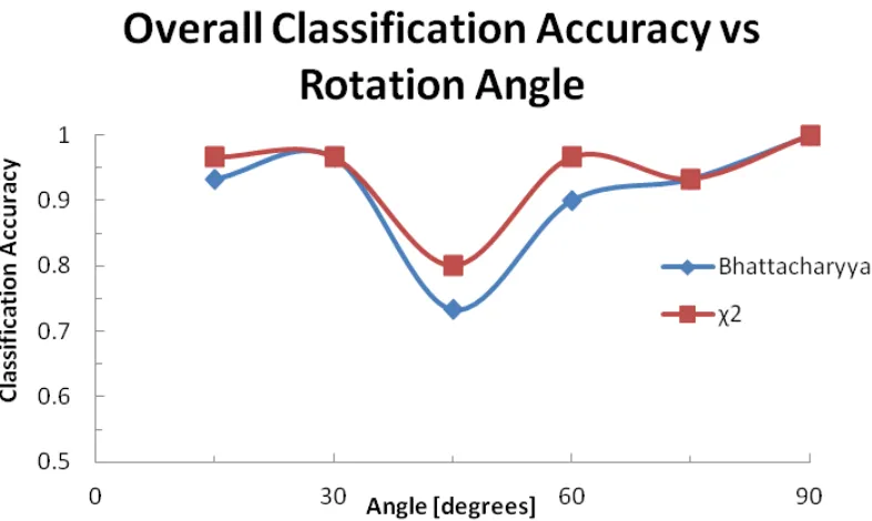
Both the Brodatz and Curet databases described above were used to tune the classifier’s free parameter, the bandwidth, as well as test the two minimum classification methods

-the Bhattacharyya and χ2 distances. The Brodatz database was used to test the classi-fier’s invariance to rotation, and the Curet database was used to test the several ways of incorporating color content into the feature set.

3.3.1 Database Setup

Brodatz

The 30 classes from the Brodatz album chosen for these experiments are shown in Figure

3.1. These were first cropped to 512 by 512 pixel size, and for each class, six additional tiles were produced by rotating the initial orientation by 15◦. This produced a total of

seven tiles per class, identical except for orientation, which with six rotations resulted in

(53)