City, University of London Institutional Repository
Citation
: Allefeld, C. ORCID: 0000-0002-1037-2735, Goergen, K. and Haynes, J-D.
(2016). Valid population inference for information-based imaging: From the second-level t-test to prevalence inference. Neuroimage, 141, pp. 378-392. doi:10.1016/j.neuroimage.2016.07.040
This is the accepted version of the paper.
This version of the publication may differ from the final published
version.
Permanent repository link:
http://openaccess.city.ac.uk/id/eprint/22843/Link to published version
: http://dx.doi.org/10.1016/j.neuroimage.2016.07.040
Copyright and reuse:
City Research Online aims to make research
outputs of City, University of London available to a wider audience.
Copyright and Moral Rights remain with the author(s) and/or copyright
holders. URLs from City Research Online may be freely distributed and
linked to.
City Research Online: http://openaccess.city.ac.uk/ [email protected]
Valid population inference for
information-based imaging:
From the second-level
t
-test
to prevalence inference
Carsten Allefelda* Kai Görgena John-Dylan Haynesa,b**
a. Bernstein Center for Computational Neuroscience, Berlin Center of Advanced Neuroimaging, Department of Neurology, and Excellence Cluster NeuroCure, Charité – Universitätsmedizin Berlin, Germany
b. Berlin School of Mind and Brain and Department of Psychology, Humboldt-Universität zu Berlin, Germany
Address for all affiliations: Charité-Campus Mitte, Philippstr. 13, Haus 6, 10115 Berlin, Germany
* E-mail: [email protected] ** E-mail: [email protected]
Corresponding author: Carsten Allefeld, Tel. +49 30 2093 6766
preprint of
C. Allefeld, K. Görgen, J.-D. Haynes. Valid population inference for information-based imaging: From the second-levelt-test to prevalence inference.NeuroImage, 141: 378–392, 2016. doi:10.1016/j.neuroimage.2016.07.040
this version includes minor fixes and a note added after publication 2016-8-10
Abstract
In multivariate pattern analysis of neuroimaging data, ‘second-level’ inference is often performed by entering classification accuracies into at-test vs chance level across sub-jects. We argue that while the random-effects analysis implemented by thet-test does provide population inference if applied to activation differences, it fails to do so in the case of classification accuracy or other ‘information-like’ measures, because the true value of such measures can never be below chance level. This constraint changes the meaning of the population-level null hypothesis being tested, which becomes equiva-lent to the global null hypothesis that there is no effect in any subject in the population. Consequently, rejecting it only allows to infer that there are some subjects in which there is an information effect, but not that it generalizes, rendering it effectively equivalent to fixed-effects analysis. This statement is supported by theoretical arguments as well as simulations. We review possible alternative approaches to population inference for information-based imaging, converging on the idea that it should not target the mean, but the prevalence of the effect in the population. One method to do so, ‘permutation-based information prevalence inference using the minimum statistic’, is described in detail and applied to empirical data.
Keywords
information-based imaging, multivariate pattern analysis, t-test, population inference, effect prevalence
1
Introduction
Since the seminal work of Haxby et al. (2001), an increasing number of neuroimaging studies have employed multivariate methods to complement the established mass-univariate approach (Friston et al., 1995) to the analysis of functional magnetic reso-nance imaging (fMRI) data, a field now known as multivariate pattern analysis (MVPA; Norman et al., 2006). Most MVPA studies use classification (Pereira et al., 2009) to exam-ine activation patterns; the accuracy of a classifier in distinguishing activation patterns associated with different experimental conditions serves as a measure of multivariate effect strength. Since the target of MVPA is not a generally increased or decreased level of activation but theinformation contentof activation patterns (cf. Pereira and Botvinick, 2011), it has also been characterized as information-based imaging and distinguished from traditional activation-based imaging (Kriegeskorte et al., 2006).
In univariate analysis of multi-subject fMRI studies, the standard way to achieve population inference is to perform a ‘second-level’ null hypothesis test (Holmes and Friston, 1998). For each subject, a ‘first-level’ contrast (activation difference) is computed, and this contrast enters a second-level analysis, at-test or an ANOVA. Specifically for a simple one-sidedt-test vs 0, reaching statistical significance allows to infer that the experimental manipulation is associated with an increase of activation on average in the population of subjects. This is interpreted in such a way that the effect is ‘common’ or ‘stereotypical’ in that population (Penny and Holmes, 2007, p. 156).
With the adoption of information-based imaging, it has become accepted practice to apply the same second-level inferential procedures to the results of first-level multivari-ate analyses, in particular classification accuracy (see e.g. Haxby et al., 2001; Spiridon and Kanwisher, 2002; Haynes et al., 2007): A classifier is trained on part of the data and is tested on another part, using each part for testing once (cross-validation), and the classification performance is quantified in the form of an accuracy, the fraction of correctly classified test data points. Applied for example to two different experimental conditions, if there was no multivariate difference in the data between conditions, the classifier would operate at ‘chance level’, i.e. it would on average achieve a classifica-tion accuracy of 50 %. At the second level, accuracies from different subjects are then entered into a one-sided one-samplet-test vs 50 %, in order to show that the ability to classify above chance and therefore the presence of an information effect is typical in the population the subjects were recruited from.
In this paper we argue that despite of the seemingly analogous statistical procedure, at-test vs chance level applied to accuracies cannot provide evidence that the corre-sponding effect is typical in the population. In contrast to other criticisms of this use of the t-test (see below), in our view the problem is not so much that the estimation distribution of cross-validated accuracies is not normal or even symmetric, or that a normal distribution model is generally inadequate for a quantity bounded to an interval[0 %, 100 %]. Rather, the problem is that other than estimated accuracies, the
true single-subject accuracy can never be below chance levelbecause it measures an amount of information.1We will show that this restriction changes the meaning of thet-test: It now tests the global null hypothesis (Nichols et al., 2005) that there isno information in any subject in the population. As a consequence, achieving a significant test result allows us only to infer thatthere are people in which there is an effect, but not that the presence of information generalizes to the population. The argument does not only hold for classification accuracy, but also for other ‘information-like’ measures.
The t-test on accuracies has been criticized before (Stelzer et al., 2013; Brodersen et al., 2013) on the grounds that its distributional assumptions are not fulfilled for cross-validated classification accuracies. Such a distributional error invalidates the calculation of critical values for thet-statistic and can therefore lead to an increased rate of false positives. This problem may be solved by better distribution models (Brodersen et al., 2013) or the use of non-parametric statistics (Stelzer et al., 2013). Our criticism goes
1Note that in this paper we only discuss the standard case of MVPA where the pair of experimental
significantly beyond that: Not only is thet-test quantitatively wrong, but it effectively tests a null hypothesis that is qualitatively different from its use with univariate statis-tics, with the consequence that rejection of this null hypothesis no longer supports population inference.
Please note that our criticism pertains specifically to a second-levelt-test applied to per-subject classification accuracies or similar measures. It does not apply to the classifi-cationof subjects, e.g. into different patient groups in medical applications (Sabuncu and Van Leemput, 2012; Sabuncu, 2014), or to the classification of condition-specific pat-ternsacrosssubjects (Mourao-Miranda et al., 2005). Moreover, it only concerns quantities that measure the information content of data, but not related quantities like classifier weights (Wang et al., 2007; Gaonkar and Davatzikos, 2013; Gaonkar et al., 2015, see below).
The organization of the paper is as follows: In Part 2 we detail how a second-level t-test achieves population inference for univariate contrasts. We then explain that MVPA measures are ‘information-like’ and show, both theoretically and using simulations, that for such measures thet-test effectively tests the global null hypothesis that there is no effect in any subject. Part 3 reviews possible alternatives to thet-test on accuracies, converging on the idea that population inference for information-based imaging should target the proportion of subjects in the population with an effect. One way to implement such an ‘information prevalence inference’ is described in detail in Part 4, and results of its application to real data are compared with those of thet-test. We conclude with the discussion of a number of questions surrounding the problem of population inference for information-based imaging.
2
The problem with the
t
-test on accuracies
2.1
Population inference in univariate fMRI analysis
To see why the t-test on accuracies cannot provide population inference, we briefly recapitulate how standard univariate analysis does achieve it. In a single subject, an activation difference or contrast ∆β is estimated based on the general linear model (GLM; Friston et al., 1995). Because it is obtained from noisy data, the estimate is itself noisy,
c
∆β∼ N(∆β,σ12), (1)
whereσ12denotes theestimation varianceof the contrast (cf. Fig. 1a). If several subjects
are included in a study, the true activation difference∆βvaries across subjects (Fig. 1a):
∆βk ∼ N(∆µ,σ22) (2)
where∆µis the average true activation difference in the population of subjects andσ22
thepopulation varianceof the effect (Fig. 1b). The added subscriptkindicates that we now consider the subject as randomly sampled from the population. The estimated contrast in several subjects therefore shows variation for two reasons — they are noisy estimates (σ12), and different subjects respond differently (σ22):
c
The symbol∆βck indicates that this contrast is both estimated and sampled.
A one-sidedt-test applied to the∆βckfrom a sample of subjectsk =1 . . .Nhas the null hypothesis∆µ =0. If it can be rejected (∆µ > 0), this allows us to make a statement about the population of subjects because∆µis a parameter of apopulation model(Eq. 2). And this statement concerns a typical effect because∆µis the mean, median, and mode of the assumed normal distribution. This kind of test is also calledrandom-effects analysis
(RFX) because it treats subjects as as randomly sampled from a population (Searle et al., 1992). It was introduced into fMRI by Holmes and Friston (1998) to replace previous
fixed-effects analyses(FFX), which did not account for population variation and therefore did not provide population inference.2
2.2
The
t
-test on accuracies
Using a second-levelt-test vs chance level with classification accuracies implies that an analogous random-effects model applies: In each subject (first level) we obtain an
estimated accuracywhich varies with an estimation varianceς21,
ˆ
a ∼ N(a,ς21). (4)
The underlyingtrue accuracy a(see App. A) varies across subjects (second level) with a population variance ς22,
ak ∼ N(a¯,ς22). (5)
Therefore estimated accuracies vary across subjects with the combined varianceς21+ς22,
ˆ
ak ∼ N(a¯,ς21+ς22). (6)
Here ¯ais the average true classification accuracy in the population, and the null hy-pothesis is that this population average is at chance level, ¯a =a0. Again, the symbol ˆak indicates that this accuracy is both estimated and sampled. Though a normal distribu-tion cannot hold exactly since both ˆaandakare limited to[0 %, 100 %], we can argue that thet-test is robust against violations of normality (Rasch and Guiard, 2004).
It appears that we have a viable random-effects model to justify the application of a second-levelt-test to accuracies. But there is a problem with this simple transfer: In contrast to estimated accuracies ˆa, the true accuracyacannever be belowthe chance level
a0.
2.3
There is no negative information
To understand whya≥a0must hold, it helps to recognize that MVPA aims at a generic
kind of effect, namely,whether or not information about experimental conditions is present
2The specific RFX procedure to apply a second-levelt-test or ANOVA to first-level contrast estimates
is called the ‘summary statistic’ approach (Penny and Holmes, 2004) because it considers only the contrast estimates∆cβkwhichsummarizesingle-subject data. It is interesting to note that it is only this
c ∆β ∆β
−20 −10 0 10 20
activation difference S3 S2 S1 a) c ∆βk
∆βk
S3 S2 S1
−20 −10 0 10 20
activation difference
b)
−060−40−20 0 20 40 60 0.2
0.4 0.6 0.8 1
true activation difference∆β
mut. info rmation / bit c)
chance levela0
−60−40−20 0 20 40 60 50 60 70 80 90 100
true activation difference∆β
true accuracy a / % d) ˆ a a
0 25 50 75 100 accuracy / %
S3 S2 S1 e) ˆ ak ak S3 S2 S1
0 25 50 75 100 accuracy / %
[image:7.595.124.472.70.508.2]f)
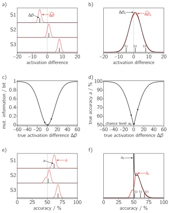
Figure 1:Distributions of true (black) and estimated (red) values of contrasts and classification accuracies. — a) An activation difference estimated from a limited amount of noisy data shows variation (red curves;σ1 =1) around the true value (black bars). Moreover, the true contrast is different in different subjects (Three panels S1, S2, S3;∆β=−5, 1, 8. Values for these subjects
are also indicated in the following panels by dots or bars.) — b) True activation differences (black bars) come from a distribution characterizing the population of possible subjects (black curve;
∆µ=1,σ2 =4). Estimated contrasts across subjects show the combined effect of both sources of variation (population + estimation, red curve;√σ12+σ22 =4.12). — c) The amount of information
single-trial data provide about the trial class (condition) and vice versa, as a function of the true activation difference. A negative contrast provides positive information. — d) True accuracy aof classification of univariate single-trial data as a function of the true activation difference. It is a symmetric function of∆β, which makes accuracy an information-like measure, with a
minimal valuea0 =50 %. — e) Estimation variation of accuracy (6-fold cross-validation) in the three subjects (red curves). As apparent for subject 2, the distributions can deviate strongly from normality. While estimated accuracies can be below chance (gray line), true accuracies (black bars;a=67.7, 51.5, 61.3 %) cannot. — f) The population variation (black curve) and combined variation (population + estimation, red curve) of accuracy that result from the population distribution of contrasts∆βk(b, black line), the functional relationship between∆βanda(d),
in the experimental data(Pereira and Botvinick, 2011). Instead of making the common distinction between univariate and multivariate fMRI analysis, we follow Kriegeskorte et al. (2006; 2007) in distinguishing between activation-based and information-based imaging. Activation-based analysis is interested in whether there is a specific change in the activation of a voxel (average BOLD signal) corresponding to an experimental manipulation, normally an increase. Information-based analysis determines whether there is any change at all, be it an increase or decrease. It looks for brain areas where the difference of conditions makes any kind of difference with respect to the fMRI signal, i.e. for information (Bateson, 1972).
Because information-based analysis disregards the sign of activation differences, it has itself an unsigned outcome: There either is a difference, then there is above-zero informa-tion, or there is no difference, then there is zero information (‘chance level’). This holds for information-theoretic measures in the strict sense (cf. Cover and Thomas, 2012), in particular mutual information (Fig. 1c), but also for the true value ofinformation-like mea-sures including averaged absolutetand Mahalanobis distance∆(used by Kriegeskorte et al., 2006), Wilks’Λ(used by Haynes and Rees, 2005b), linear discriminantt(LD-t, Nili et al., 2014), pattern distinctnessD(Allefeld and Haynes, 2014), or classification accuracya.3Thetruesingle-subject accuracy is either above chance level,a >a0, if it
is possible to extract information, or it is at chance level, a = a0, if not — but never
below (Fig. 1d).Estimatedaccuracies can be below chance, but only due to imprecise estimation ofaby ˆa, i.e. below-chance accuracies are accounted for by the first-level model of Eq. 4, not the second level of Eq. 5.
2.4
What does a
t
-test on accuracies mean?
This restriction creates a problem for the second-level null hypothesis, which qualita-tivelychanges its meaning. If
H0 : ¯a=a0 (7)
is true, then ak ∼ N(a0,ς22) (Eq. 5), which means that while half the people in the
population exhibit true above-chance classification, the other half is assumed to system-atically exhibit true below-chance classification, contradicting our insight thata ≥a0.
The null hypothesis of thet-test can only be made compatible with this constraint by ad-ditionally assuming that there is no population variation at all, H0 : ¯a= a0 ∧ ς22=0.4
And this means that the the true accuracy is at chance level for everybody,
H0 :∀k ak =a0, (8)
— there is no information inany subjectin the population. Such a null hypothesis, which is a logical conjunction of many simpler null hypotheses, has been called ‘global null hypothesis’ by Nichols et al. (2005).
3We define as ‘information-like’ those measures that covary with mutual information. Note that this
excludes other quantities that may be of interest in MVPA, in particular classifier weights (see Gaonkar and Davatzikos, 2013). Correspondingly, a classifier weight can be negative (cf. Todd et al., 2013), in the simplest case if information is coded in the corresponding voxel by a decrease in activation (but cf. Haufe et al., 2014).
4We would like to thank an anonymous reviewer for pointing out that this poses an additional
Note that this conclusion does not depend on the assumption of normality in Eq. 5 (which entered through the analogy to Eq. 2): Foranydistribution of true accuracies, if its mean is at chance but none of its realizations can be below chance, it follows that there can be no above-chance realizations either. Therefore the only possible form in which the null hypothesis formulated in Eq. 7 can hold is given by Eq. 8.
The seemingly small constraint a ≥ a0has strong consequences for inference. If the t-test allows us to reject the null hypothesis, this provides evidence for the alternative, its logical negation. Since the global null hypothesis (Eq. 8) is a universal statement, its negation is a statement of existence:
¬H0 : ∃k ak >a0. (9)
This means we have reason to believe that there are somepeople in the population whose fMRI data carry information about the experimental condition — but we have no grounds to believe that we have found an effect that istypicalin the population. The constraint onaneutralizes the RFX modeling of between-subject variation, making the
t-test applied to accuracies effectively an FFX analysis.5
Since the constraint that the true value cannot be below chance level applies to all information-like measures, the problems for population inference demonstrated here hold for information-based imaging in general. However, in the interest of conciseness our discussion focuses on cross-validated classification accuracy as the most commonly used measure in MVPA.
At this point, the main argument of this paper is concluded: The t-test on accuracies does not provide population inference, but effectively implements fixed-effects analysis. The following section further illustrates and practically demonstrates this fact using simulated data. Readers which are already convinced by the theoretical argument may skip forward to Part 3 which discusses information prevalence inference as an alternative to thet-test.
2.5
What does a
t
-test on accuracies do?
In the previous sections we gave a theoretical argument that the null hypothesis of a second-levelt-test changes its meaning under the constraint that holds for information-like measures including classification accuracy. But does this argument have practical relevance — after all, we never see ‘true accuracies’ but only estimates, whichcanbe below chance? Does our observation actually affect how at-test on accuraciesbehaves?
To investigate this question, we simulate fMRI data according to the first-level GLM (see Eq. 28) of a simplified experiment containing two experimental conditions, for a sample of subjects. A simulation is parametrized by the population mean activation difference between conditions,∆µ, and the population variationσ2(Eq. 2). The
estima-tion variaestima-tion (Eq. 1) is kept atσ1 =1. Accuracies for the classification of single-trial
data by a linear support vector machine are estimated using run-wise cross-validation,
5Todd et al. (2013) point out a related but different problem in applying a second-level test to a
−1 −0.5 0 0.5 1 0
0.5 1 1.5 2
∆µ σ2
a) t-test on accuracies
−1 −0.5 0 0.5 1
0 0.5 1 1.5 2
∆µ σ2
b) t-test on activation differences (RFX)
−1 −0.5 0 0.5 1
0 0.5 1 1.5 2
∆µ σ2
c) FFX analysis
−1 −0.5 0 0.5 1
0 0.5 1 1.5 2
∆µ σ2
d) classification across subjects
[image:10.595.71.531.76.612.2]0.05 0.1 0.2 0.5 1 rejection probability
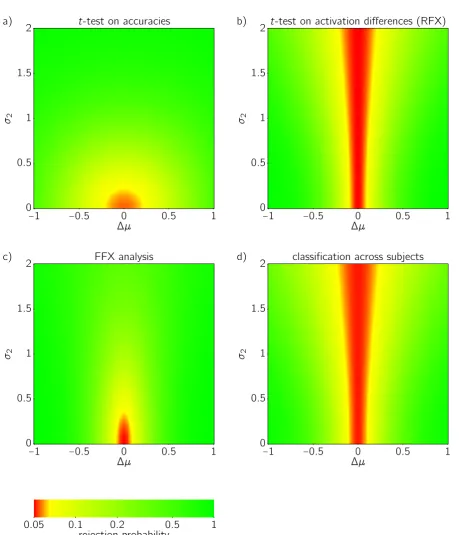
Figure 2:Rejection probability as a function of simulation parameters∆µ(the population mean
true contrast) andσ2(the population variance of true contrasts), for different null hypothesis tests at significance levelα=0.05. — a) Second-level one-sided one-samplet-test applied to
estimated classification accuracies vs chance levela0 =50 %. The smallest rejection probability is reached if both∆µ=0 andσ2 =0. — b) Second-level two-sided one-samplet-test applied to estimated activation differences vs 0 (univariate RFX analysis). The smallest rejection probability is reached for∆µ=0. — c) Fixed-effects analysis of activation differences. The smallest rejection
and these accuracies are entered into a one-sided one-sample t-test vs chance level
a0 = 50 % across subjects atα = 0.05. This is repeated many times to determine the probability to rejectthe null hypothesis. For full details of the simulations, see App. B and C.
2.5.1 Classification of univariate data with a normal population model
For simplicity, we first examine the rejection probability of thet-test on accuracies for the classification of univariate data; Fig. 1 illustrates the distributions arising in this case. The resulting rejection probability as a function of the simulation parameters∆µ andσ2is shown in Fig. 2a.
The rejection probability function is a standard tool to check whether a test is valid for a given null hypothesis and how powerful it is (Lehmann and Romano, 2005). Here, we use the function in the opposite direction: Wedefinethe test’seffective null hypothesis
as that set of parameter values where the rejection probability remains at or below the specified significance levelα.
For thet-test on accuracies (Fig. 2a) the result is that strictly there are no such parameter values: the smallest rejection probability is 0.055. This is most likely because the nor-mality assumption of Eq. 6 holds only approximately; the slight increase of theα-error
is however within the bounds used by Rasch and Guiard (2004) when stating that the
t-test is robust against violations of normality. If we disregard this deviation, the effec-tive null hypothesis turns out to be∆µ =0 ∧ σ22 =0: no population variation, and no
activation effect in any subject. This means that the true activation difference is zero in all subjects,∀k∆βk =0, and since the true accuracy corresponding to a zero activation difference is at chance level,a(∆β =0) = a0, it is equivalent to H0 : ∀k ak = a0— no
information in any subject in the population. The simulation confirms the practical relevance of our previous theoretical conclusion that thet-test on accuracies tests the global null.
For comparison, Fig. 2b shows the rejection probability function of a second-level two-sidedt-test on first-level activation differences (univariate RFX analysis). In accordance with the design of the test, its rejection probability remains at 0.05 if and only if∆µ =0, and increases monotonically with|∆µ|. Thoughσ22is not part of the specification of the
null hypothesis, we observe that for stronger population variation it becomes harder to reach a significant effect. This is in stark contrast to thet-test on accuracies (Fig. 2a), where increasingσ22makes it easier to reject the null hypothesis. The moreinconsistent
activation differences (or by extension: patterns; see below) are in the population, the more likely it is that thet-test on accuracies will indicate the presence of an information effect that is supposedly ‘typical’ in the population!6
As we noted above, univariate fixed-effects analysis does not provide population-level inference simply because its null hypothesis (that the sample mean is 0) does not reference a population distribution. We can however apply an FFX test to our simulated univariate RFX data and thereby determine the null hypothesis it effectively implements in this context. The result shown in Fig. 2c demonstrates that the effective null hypothesis of FFX analysis is∆µ =0 ∧ σ22=0. Though their rejection probability 6Davis et al. (2014) make a similar observation, but without noting its consequences for population
functions are different in detail, a t-test on accuracies and a fixed-effects analysis of activation differences operate qualitatively identical: they both detect deviations from a zero population mean contrast ∆µ as well as from a zero population variance of constrasts σ22. This agreement supports our earlier statement that even though a t
-test on accuracies formally acknowledges population variation, it does not provide population inference any more than FFX analysis does.
To complete the picture, Fig. 2d shows the rejection probability function of a test based on classification across subjects (cf. Mourao-Miranda et al., 2005). The single-subject univariate contrast estimates in each of the two conditions form the data set that is used to train and test a classifier in leave-one-subject-out cross-validation, and the distribution of accuracies is determined for different simulation parameters. For a given simulated data set the null hypothesis (true accuracy = chance level) is rejected if the accuracy reaches or exceeds the critical value of 67.6 %, which is the approximate 95th percentile of the distribution of accuracies under the null hypothesis. The result demonstrates that this test behaves in a way that is very similar to the second-levelt-test applied to the same first-level activation differences (Fig. 2b). Both provide population inference because they both implement the null hypothesis ∆µ = 0 for arbitrary population variance σ22.
The difference is that while the second-levelt-test is limited to univariate contrasts, the test based on classification across subjects can just as well be applied to multivariate data, where the null hypothesis becomes∆~µ =~0. If a significant effect is found, this
provides evidence that there is apattern difference∆~µthat is typical in the population.
Since this implies that the presence of information is typical in the population, it appears that the problem of population inference for information-based imaging could simply be solved by applying classifiers or other MVPA methods always across subjects. Unfortunately, spatial normalization algorithms do not achieve precise voxel-level anatomical alignment (Thirion et al., 2006), and moreover we cannot assume that a one-to-one correspondence of informative patterns between subjects always exists (Haynes and Rees, 2006; Kriegeskorte and Bandettini, 2007; Haxby, 2012), so that classification across subjects is often bound to fail for a trivial reason.7
2.5.2 Classification of multivariate data with a normal population model
An important observation in the last section was that the larger the population variance
σ22, i.e. the more inconsistent activation differences are across subjects, the easier it
becomes for thet-test on accuracies to achieve significance. To make sure that this effect is not limited to univariate data, Fig. 3a shows the rejection probability function for different numbers of dimensions, p=1, 2, and 10. Data are generated as before, but for
pdifferent voxels in parallel, with both first- and second-level variation uncorrelated between voxels. Accordingly, the classifier is trained and tested in a p-dimensional space. To facilitate visualization, we kept the population mean activation difference at zero in all voxels, ∆µ = 0. The result demonstrates that the effect of population
7A solution might be provided by ‘hyperalignment’ (Haxby et al., 2011) which attempts to establish
p= 1
p= 2
p= 10
0 0.5 1 1.5 2 0
0.2 0.4 0.6 0.8 1
σ2
rejection
probabilit
y
a)
∆β∗= 1
∆β∗= 2 ∆β∗= 5
0 0.2 0.4 0.6 0.8 1 0
0.2 0.4 0.6 0.8 1
γ
rejection
probabilit
y
[image:13.595.78.523.72.245.2]b)
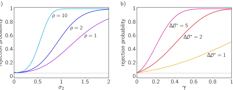
Figure 3:Rejection probability of a second-level one-sided one-samplet-test applied to esti-mated classification accuracies vs chance level, as a function of simulation parameters. The significance level α = 0.05 is shown as a gray horizontal line. — a) Multivariate normally
distributed contrasts in pvoxels, with variation uncorrelated between voxels and a population mean activation difference of∆µ=0 everywhere. The rejection probability increases with the
population varianceσ22, and the increase is stronger for higher dimensionality p. The line for
univariate data (p=1) corresponds to a central vertical section through the rejection probability function of Fig. 2a. — b) Population proportion model: Fixed true contrast∆β∗in a proportion γof the population, and 0 in the rest. The rejection probability always reachesαforγ=0.
variance on the rejection probability stays qualitatively the same, but is even stronger in higher dimensions. We can therefore assume that the effective null hypothesis of the t-test on accuracies generalizes from the univariate ∆µ = 0 ∧ σ22 = 0 to the
multivariate ∆~µ =~0 ∧ Σ2 = 0, where Σ2 is the multivariate population variance
(variance–covariance matrix). That implies ∀k ∆~βk = ~0 — there is no informative pattern in any subject in the population — which is again equivalent to H0 : ∀k ak =a0,
the global null.
2.5.3 Classification of univariate data with a population proportion model
Our simulation-based finding that the effective null hypothesis of at-test applied to first-level accuracies is H0 : ∀k ak =a0(the global null) was so far obtained using the
standard normal distribution population model for activation differences (Eq. 2), which may not be correct (cf. Rosenblatt et al., 2014). With respect to true accuracies, this model for true contrasts has a peculiar consequence: As soon as there is any population variation, i.e.σ22 >0, the probability that the true contrast in a given subjectkis exactly ∆βk =0 becomes zero, which implies that almost always ∀k ∆βk 6=0. Since for non-zero true contrast the true accuracy is above chance,a(∆β6=0) >a0(cf. Fig. 1d), this
further implies that almost always∀k ak > a0. Therefore the assumption of a normal
population distribution of activation differences allows only two possibilities: Either there is no information in the data ofanysubject (the effective null hypothesis), or there is information in the data ofeverysubject. There is nothing in between.
from Rosenblatt et al., 2014): Assume that the true contrast has a fixed value∆β∗in a certain proportionγ∈ [0, 1]of the population and the fixed value 0 in the rest. If now a
subjectkis randomly selected from the population, this means that
∆βk =
0 with probability 1−γ ∆β∗ with probability
γ . (10)
Fig. 3b shows the behavior of thet-test in a simulation using this model. The result is that for different values of∆β∗, the rejection probability reaches the significance levelα
always atγ =0. This effective null hypothesis is again equivalent to the global null,
H0 : ∀k ak = a0. Moreover, the simulation demonstrates that thet-test on accuracies
may with high probability declare an information effect to be ‘typical’ even though it is only present in a small minority of subjects in the population!
3
An alternative: Information prevalence inference
In the previous part we established that the second-levelt-test applied to accuracies is not able to provide population inference. We now discuss alternative approaches, leading us to the idea that population inference for information-based imaging should target theproportionof people in the population in which there is an information effect.
Within the MVPA literature, there are three alternative proposals. First, Kriegeskorte and Bandettini (2007) recommend to apply the methods for ‘combining brains’ collected by Lazar et al. (2002). However, except for the summary-statistic approach of Holmes and Friston (1998), all of these methods8are meta-analytic procedures which explicitly test the global null. Second, Stelzer et al. (2013) propose to generate single-subject permutation statistics, and then to construct a second-level permutation distribution by randomly selecting first-level permutations in each subject. Because each permutation realizing the second-level null hypothesis is a combination of permutations realizing the first-level null hypotheses in every subject, this again tests the global null hypothesis of no information in any subject. And third, Brodersen et al. (2013) follow Olivetti et al. (2012) and Brodersen et al. (2012) in describing a mixed-effects analysis for MVPA, introducing explicit estimation and population models for classification accuracies. This approach offers several improvements over thet-test on accuracies: Their model can account for different estimation variances (ς21) in different subjects, and it uses more
realistic distributional assumptions. However, the authors do not consider the fact that true accuracies are limited to the range[a0, 1](for binary classification:[50 %, 100 %]).
Unfortunately, this renders their approach only an improved version of thet-test on accuracies.
As detailed in Sec. 2.4, the flaw of the t-test on accuracies lies in the fact that the distributional assumption of the underlying second-level model (Eq. 5) is incompatible with the restriction a ≥ a0, unless ς2 = 0. This could conceivably be fixed by using
another population model which adheres to that restriction by design. However, the simulated population distribution of true accuracies for univariate classification in
8Fisher’s (1925) combined probability test, Tippett’s (1931) minimump-value, the conjunction test of
Fig. 1f does not look like it could be appropriately captured by a parametric model. And even if that were the case, the distribution would likely have a different shape for classification in higher dimensions or for multi-class classification. It might additionally depend on the specific classification algorithm, and it would certainly be different again for other information-like measures.
Moreover, inference with respect to the population mean is generally inadequate for information-like measures no matter how well the actual population distribution can be modeled. The reason is that the true mean is above chance as soon as there is a true above-chance effect in a small fraction of the population (cf. Fig. 3b; because there can be no true below-chance effect). This problem can be resolved by inference that does not target the mean effect, but the proportion of subjects in the population in which there is an information effect, i.e. theprevalenceof information.
Such an approach is followed by Rouder et al. (2007) in the context of signal detection theory with their ‘mass-at-chance model’. They assume a probit-normal population distribution of true detection accuracies, which however is truncated at 50 %, such that all subjects that are nominally below chance are instead located at chance. Inference with respect to the prevalence of an effect has also been advocated by Rosenblatt et al. (2014) for mass-univariate analysis. The authors argue that imperfect alignment of single-subject activation maps leads to areas where only a subset of subjects have a non-zero activation, and propose to replace the standard normal population model (Eq. 2) by a mixture model. We used a simplified version of this in the population proportion simulation (Eq. 10 and Fig. 3b). Stephan et al. (2009) propose a Bayesian form of prevalence inference as RFX analysis for dynamic causal models (DCM), ex-tending first-level model selection to a posterior distribution over the space of different model frequencies. In a specific application this discrete distribution may describe the distinction between a zero effect and a generic non-zero effect.9Friston et al. (1999a) build upon their previous idea of a conjunction test (Price and Friston, 1997; Worsley and Friston, 2000) and introduce the minimum-statistic approach. Their analysis pro-ceeds in two steps: first, the minimum statistic is used to derive a p-value for the null hypothesis that there is no effect in any subject in the population, the global null. In a second step, a correction is applied that allows to test the null hypothesis that the proportion of subjects in which there is an effect,γ, is at or below a thresholdγ0. The
rejection of this null hypothesis therefore allows to infer thatγ >γ0.
The approaches of Rouder et al. (2007), Rosenblatt et al. (2014), Stephan et al. (2009), and Friston et al. (1999a) are all candidates to be adapted for information-based imaging, to provide population inference with respect to the prevalence of an information effect. In the following we demonstrate this in detail for the method of Friston and colleagues.
9Stephan et al.’s Bayesian RFX analysis for DCM has been adapted for GLM model selection by Soch
4
Permutation-based information prevalence inference
using the minimum statistic
In this part we recapitulate the minimum-statistic approach to prevalence inference developed by Friston et al. (1999a), adapt it to be based on permutation statistics, and detail the resulting algorithm. Applied to information-like measures this method allows us to achieveinformation prevalence inference, i.e. inference with respect to the proportion of subjects in the population that exhibit an information effect. We demonstrate the method using an example data set.
The advantage of Friston et al.’s approach is that it can be implemented based on known permutation methods at the single-subject level (Golland and Fischl, 2003; Etzel and Braver, 2013; Schreiber and Krekelberg, 2013; Stelzer et al., 2013; Allefeld and Haynes, 2014; see also Ernst, 2004). The method is discussed with respect to classification accuracy, but the test logic applies equally to other information-like measures.
A note on notation: We previously used variables without index (e.g.a) when talking about the ‘first level’ of a given single subject, and symbols with index (e.g.ak) when considering a subject as randomly selected from the population, or referring to all members of the population (∀k). This notation is still followed, but we now extend it such that an index associated with an explicit range,k =1 . . .N, refers to the specific subjects included in a given sample.
4.1
The minimum statistic and the global null
In a single subject, an estimated classification accuracy ˆahas an associatedp-value p(aˆ), which is the probability to observe an accuracy that large or larger given that the true accuracy is at chance level (a =a0).
For a sample of N subjects with estimated classification accuracies ˆak, k = 1 . . .N, we choose theminimum statistic(smallest observed accuracy) as the second-level test statistic,
m=minN
k=1 aˆk. (11)
As a second-level null hypothesis we first consider theglobal null hypothesis,
H0 :∀k ak =a0, (12)
that there is no effect in any subject in the population. In order to test this null hypothe-sis, we need the p-value ofm, pN(m), with respect to the global null.
To say that the minimum of estimated accuracies is at or larger than a given value mis the same as saying that all of the estimated accuracies ˆak,k =1 . . .N, are at or larger thanm. Since subjects are independently drawn from the population, the probability to observe a minimum ofmor larger under the global null is the product of probabilities to observe an estimated accuracy ofmor larger in each subject in the sample:
pN(m) = N
∏
k=1where p(m)is the single-subjectp-value for ˆa =m.
If pN(m) ≤ α, then we can reject H0 and infer that there are some subjects in the
population in which there is an above-chance effect. Since this is a statement of existence, this does not provide evidence that the effect is typical in the population.
4.2
The prevalence null
We now consider a population model which contains the global null as a special case: The information effect targeted by the classification procedure has aprevalenceγ, i.e. a
proportion γ ∈ [0, 1] of subjects in the population have an above-chance effect, the
others no effect. If a subjectkis selected at random from this population, then
ak =a0 with probability 1−γ,
ak >a0 with probabilityγ. (14)
This is similar to the population proportion model for activation differences used above (Eq. 10), but in contrast no assumption is made about the size and distribution of above-chance effects.
An estimated accuracy ˆa in a single subject can be larger than or equal to m either purely by chance (p(m), with probability 1−γ) or because there is actually an effect
in that subject (p(m|a>a0), with probabilityγ). The probability to observe a sample
minimum ofmor larger if the prevalence isγis therefore
pN(m|γ) =
N
∏
k=1[(1−γ) p(m) +γp(m|a>a0)]
= [(1−γ) p(m) +γ p(m|a>a0)]N.
(15)
Here p(m|a> a0)is the probability to observe an estimated accuracy ofmor larger in a
single subject given a true accuracy ofa, where we only know thata >a0. Because the
size of the above-chance effecta >a0is not specified, we cannot know this probability
precisely; but because it is a probability, we know that it is smaller than or equal to one,
p(m|a>a0) ≤1, and therefore
pN(m|γ) ≤[(1−γ) p(m) +γ]N. (16)
The reason we chose the minimum statistic as the second-level test statistic is that it enables us to formulate this inequality for the prevalence model, i.e. to determine a
p-value without specifying the size and distribution of above-chance effects.
The prevalence model allows us to formulate theprevalence null hypothesis,
H0 : γ≤γ0, (17)
that the prevalence is smaller than or equal to a threshold prevalenceγ0. The global
null (Eq. 12) is a special case of the prevalence null whereγ0 =0.
test statistic is the probability to observe the given value or larger,maximizedover all situations consistent with H0. Therefore
pN(m|γ≤γ0) = [(1−γ0) p(m) +γ0]N. (18)
In a permutation approach, pN(m)can be more precisely determined thanp(m)(see step 3 under Algorithm). We therefore express the prevalence nullp-value pN(m|γ≤ γ0) in terms of the global null p-value pN(m), using the relation pN(m) = p(m)N (Eq. 13):
pN(m|γ≤γ0) = [(1−γ0) N
q
pN(m) +γ0]N. (19)
If pN(m|γ ≤ γ0) ≤ α, then we can reject H0 and infer that the prevalenceγ is
sig-nificantly larger than γ0, i.e. more than a proportion γ0 of the population have an
effect.
As an alternative to fixing a threshold prevalenceγ0in advance and then testing the
cor-responding prevalence null, we can compute the largestγ0such that the corresponding
null hypothesis can still be rejected at the given significance levelα:
γ0 =
N
√
α− pN pN(m) 1− pN p
N(m)
. (20)
Note that this is not an estimator for the true prevalenceγ, but]γ0, 1]is a one-sided
(1−α)-confidence interval for it.
This confidence interval will often be too wide because of the inequality used above (Eq. 16). Moreover, even for the strongest possible effect (pN(m) = 0) it holdsγ0 = N
√
α,
meaning that the strength of the population inference is limited by the number of subjectsNand the chosen significance levelα.
4.3
Information maps
So far we have considered a single second-level test based on classification accuracies ˆ
akfrom Ndifferent subjects. But in a common variant of MVPA, searchlight analysis (Kriegeskorte et al., 2006), we havemapsof classification accuracies and perform a test at each voxel in these maps, i.e. we have to adjust for multiple comparisons.
To do so, we need to specify aspatially extendedversion of the prevalence null. Again following Friston et al. (1999a), our spatially extended null hypothesis is:
— there is an effect with prevalenceγ ≤γ0in a small area,
— and no effect everywhere else.
The justification for this is that in experiments investigating the localization of in-formation we normally expect this inin-formation to be restricted to specialized brain areas.
Here p∗N(m)is thep-value for the spatially extended global null, corrected for multiple comparisons using a standard method (see step 4 under Algorithm). Taken together, the probability to observe a sample minimum ofmor larger at a given voxel, corrected for multiple comparisons according to the spatially extended prevalence null hypothesis is
p∗N(m|γ ≤γ0) = p∗N(m) + [1−p∗N(m)] pN(m|γ ≤γ0). (21)
For given threshold γ0, the spatially extended prevalence null can be rejected at a
particular voxel if p∗N(m|γ≤γ0)≤α. Equivalently, we can define a significance level
that is corrected for multiple comparisons,
α∗ = α−p
∗ N(m)
1−p∗N(m), (22)
and reject the spatially extended prevalence null if the uncorrected p-value is at or below the corrected level, pN(m|γ ≤γ0) ≤α∗. Note that becausemis voxel-specific, α∗is, too.
Again, we can alternatively compute the largestγ0such that the corresponding spatially
extended prevalence null can still be rejected:
γ∗0 = N
√
α∗− pN pN(m) 1− pN
pN(m)
, (23)
which results in a map of lower confidence bounds of the prevalence of the effect, an
information prevalence map.
4.4
Algorithm
We now explain in detail how the computations derived above can be implemented based on first-level permutation statistics.
Step 1: For each subject, classification accuracies ˆav are computed for each voxel v. Additionally, classification accuracies are computed for data where the class labels have been permuted, ˆavi withi = 1 . . .P1, where P1 is the number of available first-level
permutations.i =1 denotes the neutral permutation, i.e. ˆav1 =aˆv.
Step 2: The minimum classification accuracymvacross subjects (Eq. 11) is computed at each voxelv. Additionally, the minimum accuracy is computed for each second-level permutation,mvj withj=1 . . .P2. A second-level permutation is a combination of
first-level permutations, and therefore there areP1N possible second-level permutations. If there are too many combined permutations, a subset can be selected randomly (Monte Carlo estimation), but it has to be made sure that j = 1 denotes the combination of first-level neutral permutations (i = 1 in all subjects). This procedure of combined permutations is identical to the one employed by Stelzer et al. (2013).
Step 3: The uncorrected p-value for the global null hypothesis is determined at each voxel (Eq. 13) as
pN(mv) = 1
P2
P2
∑
j=1where the so-called Iverson bracket[·]has the value 1 for a true condition and the value 0 for a false condition. That is,pN(mv)is the fraction of combined-permutation values of the minimum statistic larger than or equal to the actual value. Becausemv1 = mv, the smallest possible p-value is P1
2.
Step 4: To correctpN(mv)for multiple comparisons, the maximum statistic across voxels is computed for each combined permutation (see Nichols and Holmes, 2001),
Mj =max
v mvj, (25)
and then
p∗N(mv) = 1
P2
P2
∑
j=1[mv ≤Mj] (26)
is determined.p∗N(mv)is the p-value for the spatially extended global null hypothesis. Step 5a: To determine where the spatially extended prevalence null hypothesis for a given thresholdγ0can be rejected, at each voxel Eq. 19 is used to computepN(mv|γ≤ γ0)frompN(mv), Eq. 21 to compute p∗N(mv|γ ≤γ0)from p∗N(mv)and pN(mv|γ ≤γ0),
and it is checked whetherp∗N(mv|γ≤γ0)≤α.
Step 5b: Alternatively, to determine for each voxel the largest thresholdγ0∗at which the
spatially extended prevalence null hypothesis can be rejected, Eq. 22 is used to compute
α∗vfrom p∗N(mv). ThenpN(mv) ≤α∗vis checked to see whether the spatially extended global null hypothesis can be rejected. If that is not the case, the largest thresholdγ∗0
is not defined for that voxel (the prevalence null cannot be rejected, even at γ0∗ =0).
For all voxels where the spatially extended global null hypothesis can be rejected, Eq. 23 is used to computeγ∗0v fromαv∗ andpN(mv). Note that the maximally possible
γ0∗vdetermined this way is limited not just by the chosen significance levelαand the
number of subjectsN, but also by the number of second-level permutationsP2; it is
γ∗0max =
N
√
αmax∗ − N
√
1/P2
1− √N 1/P2
with α∗max=
α−1/P2
1−1/P2
. (27)
For largeP2,α∗maxis approximately equal toα.
A problem for this method may arise from the fact that both the minimum statistic underlying prevalence inference and the maximum statistic used to correct for multiple comparisons do not produce new values (unlike e.g. the mean, which in general differs from all the values it is calculated from). Since the number of possible classification accuracies is limited because of a limited number of data points, this may lead to a large number of permutations where the statistic attains the same value (tied permutation values), which inflates the p-values computed in steps 2 and 3 above. This problem can be solved by using spatially smoothed accuracy maps as inputs (which is also advisable to reduce residual anatomical misalignment between subjects), or by using a continuously-valued information-like measure like pattern distinctness (Allefeld and Haynes, 2014) instead.
4.5
Application
belonging to four different categories were presented either to the left or the right of fixation (24 experimental conditions) to N = 12 subjects. There were four different trials per condition in each of five different runs. fMRI data were recorded from a field of view covering the ventral visual cortex at an isotropic resolution of 2 mm. Data were preprocessed and normalized to the MNI template. A linear SVM with parameter
C = 1 was trained on GLM parameter estimates from four of the runs, and tested on the fifth run, in a leave-one-run-out cross-validation scheme. Classification was pairwise (24·23 / 2=276 pairs) and accuracies were averaged across pairs combining different factor levels, so that the chance-level accuracy wasa0 =50 %. For permutation
statistics, class labels were exchanged in each of the five runs separately, which lead toP1 =25−1=16 unique first-level permutations. The analysis was performed using
a searchlight of radius 4 voxels (comprising 257 voxels). The resulting accuracy maps were smoothed with a Gaussian kernel of 6 mm FWHM. For more details, see Cichy et al. (2011) and Allefeld and Haynes (2014). For information prevalence inference, we randomly selectedP2=107out ofP1N =2.8·1014 possible combined permutations at
the second level. All the following results are corrected for multiple comparisons, but for simplicity we omit the superscript ’∗’.
x= 32
prevalence γ0
a)
0 0.2 0.4 0.6 0.8 1
median accuracy / % b)
50 60 70 80 90 100
t-value c)
[image:21.595.79.512.332.486.2]0 5 10 15 20 25
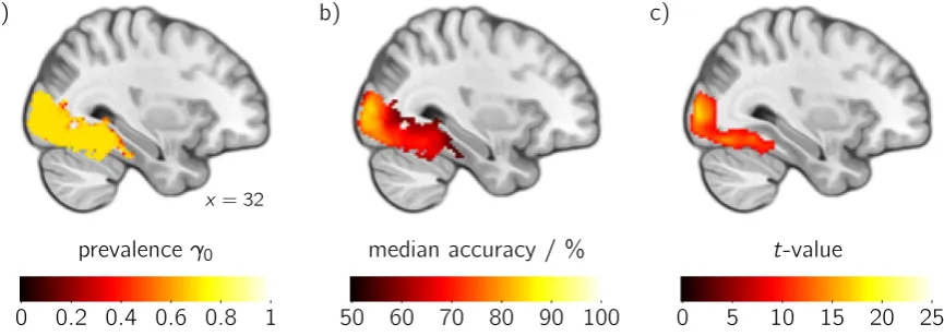
Figure 4:Second-level results for the classification of object category of a visual stimulus (see Cichy et al., 2011) shown in a sagittal slice through right lateral occipital cortex and fusiform gyrus. Statistics are corrected for multiple comparisons. — a) Information prevalence inference. Highlighted areas are those where the global null hypothesis (prevalence γ = 0) can be
rejected at a level ofα=0.05. Colors visualize a lower boundγ0on the prevalence of category information (confidence level 0.95). — b) For those areas where the prevalence null hypothesis
γ≤γ0can be rejected atγ0=0.5, i.e. where it can be inferred that the majority of subjects in the population have an effect, colors visualize the median classification accuracy across subjects. — c)t-test on accuracies vs chance levela0=50 %. For those areas where the null hypothesis
¯
a =a0can be rejected at a level ofα=0.05, colors visualize the underlyingt-value.
The results for the classification of stimulus category are shown in Fig. 4. The spatially extended global null hypothesis of no information in any subject in the population can be rejected at a level ofα =0.05 in about 27 % of in-mask voxels. For those voxels, the
largest lower boundγ0at which the spatially extended prevalence null hypothesis can
be rejected is shown in Fig. 4a. In about half of those voxels,γ0reaches the maximally
possible value (for the given sample size N, significance levelα, and number of
second-level permutationsP2) ofγ0max =0.701 (Eq. 27).
i.e. where we can infer that in themajorityof subjects in the population the data contain information about the stimulus category, the median estimated accuracy is shown in Fig. 4b. We chose the median across all subjects in the sample as a descriptive statistic to accompany our prevalence results, because it can be considered as a cautious and robust estimator of the typical above-chance classification accuracy.10
For comparison, the result of a second-level t-test on accuracies vs chance level is shown in Fig. 4c. Although the effective null hypothesis of this test is identical to the global null hypothesisγ = 0 explicitly tested in Fig. 4a, the number of voxels at
which it can be rejected is much smaller (about 14 % of in-mask voxels at α = 0.05,
FWE-corrected), indicating that in this case thet-test is less sensitive. The picture is the same for the comparison with the test of the prevalence null hypothesisγ≤γ0at γ0 =0.5 shown in Fig. 4b. Information prevalence inference therefore allows us to draw
conclusions that are stronger than those provided by thet-test on accuracies, concerning both interpretation — population inference — and, for this data set, statistical power. However, the result of Fig. 4b also calls into question whether the assumption that an effect is constrained to a ‘small area’ (adopted from Friston et al., 1999a) is generally adequate.
5
Discussion
In this paper we have shown that thet-test on accuracies commonly used in MVPA studies is not able to provide population inference because the true single-subject accuracya can never be below chance level. This constraint makes the effective null hypothesis of the test the global null hypothesis that there is no effect in any subject in the population, which means that in rejecting that null hypothesis we can only infer that there are some subjects in which there is an effect. This is in stark contrast to the standard interpretation of a significant result of a second-level t-test. We supported our statement both by theoretical arguments, in particular detailing that classification accuracy in MVPA is an information-like measure, as well as by simulations of the rele-vant distributions to investigate the practical behavior of the t-test applied to accuracy data. Finally, we reviewed possible alternative inference methods and described one approach that can be implemented based on known first-level permutation statistics in combination with the minimum statistic as the second-level test statistic. In the following we discuss a number of possible counter-arguments and questions.
Does this mean that the t-test fails, is not robust enough?— Not really. In all the instances we examined, thet-test does what it is supposed to do: Check whether the population mean is increased. The point is that under the constrainta≥ a0, rejecting H0: ¯a=a0
no longer tells us that the effect is typical in the population; an increased accuracy in a small fraction of the population is sufficient to increase the population mean (cf. Fig. 3b). Average information content is not typical information content. Concerning robustness,
10For
γ > 0.5 we can consider subjects where the true accuracy is at chance (no information) as
for the case we simulated (Fig. 2a) theα-error was only slightly increased, consistent
with the notion that thet-test is indeed robust.
Is it wrong to test the global null hypothesis?— No. The decision which null hypothesis to test rests with the researchers performing a study. The problem lies with the inter-pretation of a significant result, which for second-level analysis — at least tacitly — is to infer that the effect is typical in the population. Moreover, the step from sample to population inference (FFX to RFX) as the gold standard has been taken already a long time ago for univariate analyses (Holmes and Friston, 1998) and more recently for DCM (Stephan et al., 2009); it would therefore be natural to expect that it also becomes the standard for information-based imaging. In particular, any claim that MVPA is more sensitive than univariate analysis (Norman et al., 2006) is meaningless if MVPA is not held up to the same inferential standards.
We observe below-chance accuracies all the time.— There are two aspects to this. For one, our statement that accuracies cannot be below chance refers to true accuracies, not to estimated accuracies. Second, it is sometimes the case that estimated accuracies strongly suggest that the true accuracy is below-chance, too.11This is most likely due to the circumstance that a crucial assumption of cross-validation is not met, namely that the different parts of the data (here: fMRI recording sessions) come from the same distribution (Efron and Tibshirani, 1994). If there are systematic changes across data parts, for example because of a confound either in the data or in the experimental design (Görgen et al., 2014), this can induce a negative bias, including the possibility that classifier performance lies systematically below chance. (For another tentative explanation, see Kowalczyk, 2007.) This does of course not mean that now there is ‘negative information’, but only that cross-validated accuracy is not a meaningful information measure under such circumstances. This possibility does not invalidate the argument made in this paper, but points to another problem that needs a separate remedy.
A classifier could be designed to systematically give the wrong answer, leading to a true accuracy below chance.— Yes, but in that case the accuracy of this classifier would no longer be a measure of the information content of the data. For example in the simple case where the output of a working classifier is falsified by always returning the opposite classification result (A instead of B and B instead of A), information content would no longer be quantified bya−a0, but by−(a−a0). The argument in this paper does
not refer to classifiers in general, but to the use of classification accuracy and other measures to quantify the information content of data.
What does it mean for an effect to be ‘typical’ in the population?— This question essentially asks about the scientific content of statistical inference at the population level. Surpris-ingly, the topic is almost never discussed in statistical scientific papers and textbooks, including those aimed at psychologists and other cognitive scientists. Our use of the term ‘typical’ was inspired by Penny and Holmes (2007), who state that in population inference ‘one is interested in what is common to the subjects’ or in a ‘stereotypical effect in the population’ (p. 156). In this paper, we use the term mainly in a negative way: An effect that is only present in a small fraction of the population can hardly be
11With respect to fMRI–MVPA, this phenomenon is informally discussed (see e.g. J. Etzel’s blog,
considered typical (or ‘common’, or ‘stereotypical’). In standard univariate analysis concerning the mean of a normal distribution population model, a positive use of the term can be motivated by the fact that the mean is also the mode of the distribution (the most frequent realization) as well as its median (the value that sits ‘in the middle’ of the distribution). But there is another aspect: If in this context we can reject the null hypothesis H0 : ∆µ = 0 in a one-sided t-test, the inference ∆µ > 0 also means that
more than half of the population — the majority — have a positive effect (and less than half a negative effect). This statement can be extended to the non-normal case if there is a test that can show that the populationmedianis above zero. If we take this observation as a guideline, the natural choice for the threshold in prevalence inference isγ0=0.5 (see also Friston et al., 1999b). If we can reject this null hypothesis, we can
again infer that there is an effect in the majority of subjects in the population, which also implies that the median true effect strength is above-chance (motivating Fig. 4b).12 We therefore propose to call an effect ‘typical’ if it is present in the majority of subjects in the population.
But don’t we want to show that the effect generalizes in the sense that it is present in every subject in the population?— Maybe ideally, but in practice this is impossible. First, it is not known whether any of the effects that are of interest in functional neuroimaging do actually exhibit such an extreme degree of generalization, in particular with respect to a specific anatomical location. Second, statistical inference is unable to provide support for such a statement on principle. As pointed out above, a univariate one-sided
t-test for a normal distribution only provides evidence that a majority of subjects in the population have an effect, not that it generalizes to everyone. And in population prevalence inference, at best we could test the prevalence null hypothesis forγ0=0.99
or similar, at the price of very low sensitivity.
Concluding we would like to point out that we do not consider the method of ‘permutation-based information prevalence inference using the minimum statistic’ put forward in the last part to be the definitive solution to the problem of population inference in information-based imaging. The main aim of this paper was to demonstrate conclusively that thet-test on accuracies does not provide population inference, and that prevalence inference is an alternative. This particular method was presented in order to show that population inference is possible, even based on established methodology only (minimum statistic, first-level permutations). However, it does have several shortcomings: The use of the minimum statistic limits the highestγ0for which
the prevalence null hypothesis can be rejected depending on the number of subjects, and the permutation-based implementation imposes an even lower limit depending on the number of second-level permutations that can be performed. Moreover, this method does not provide a way to estimate (instead of just bound) the true population prevalenceγ. We do however believe that methods focusing on population prevalence
are the most promising approach, not just for information- but also for activation-based imaging, because they explicitly provide information about thedegreeto which an effect generalizes. And while we hope that this paper will motivate further methodological work on population inference for information-based imaging, our method does provide
12Additionally, this choice is consistent with the use of the ‘exceedance probability’ in Bayesian RFX
a way to improve upon the commonly usedt-test on accuracies that is available now.13
Acknowledgments
Kai Görgen was supported by the German Research Foundation (DFG grants GRK1589/1 and FK:JA945/3-1).
The authors would like to thank Tom Nichols, Jakob Heinzle, Jörn Diedrichsen, Will Penny, María Herrojo Ruiz, Joram Soch, Martin Hebart, Jo Etzel, Yaroslav Halchenko, and Thomas Christophel for discussions, comments, and hints.
Appendix
A
What is a true accuracy?
The first-level model (Eq. 4) for the RFX analysis of accuracies assumes that there is a ‘true accuracy’athat underlies the random estimated accuracies ˆathat we actually observe. But what does this true value stand for?
In the case of a true activation difference∆β, the answer is simple: The first-level GLM
yt =βAxAt+βBxBt+et (28)
wherexAt andxBt are regressor functions andet is noise, provides a statistical descrip-tion of the (neural and hemodynamic) process by which we assume the observed fMRI data are generated (a generative model). This model includes parametersβAand βB
which govern the generative process, and which characterize the respective subject. From a given data setyt, we can estimate these parameters, ˆβA and ˆβB, but because the
data are noisy, these estimates will not coincide with the underlying true values. How-ever, if we could repeat the experiment an infinite number of timeswith the same subject, the mean of estimates across these repetitions would recover the true values, because the estimators are unbiased (provided the parameters are estimable). This mean is also called expectation value;hβˆAi= βA,hβˆBi = βB, and thereforeh∆βci =∆β= βB−βA (cf. Eq. 1).
For a true accuracyathe situation is not that simple, because we do not have a genera-tive model of the datayt that is parametrized bya. But, consistent with the RFX model for accuracies and in analogy to GLM parameters, we can define the true accuracy as the expectation value of estimated accuracies,a=haˆi, i.e. the mean across an infinite number of repetions of the experiment with the same subject. This true accuracyais a complex function of the true GLM parameters for the included voxels and conditions, as well as the error variance and covariance, and may also depend on the classification algorithm.
13An implementation for Matlab can be obtained from the corresponding author or at http://github.