POSITIVITY-PRESERVING DISCRETIZATION OF THE
CONVECTION-DIFFUSION-REACTION EQUATION∗
ALEJANDRO ALLENDES†, GABRIEL R. BARRENECHEA‡, AND RICHARD RANKIN§
Abstract. This work is devoted to the proposal, analysis, and numerical testing of a fully computable a posteriori error bound for a class of nonlinear discretizations of the convection-diffusion-reaction equation. The type of discretization we consider is nonlinear, since it has been built with the aim of preserving the discrete maximum principle. Under mild assumptions on the stabilizing term, we obtain an a posteriori error estimator that provides a certified upper bound on the norm of the error. Under the additional assumption that the stabilizing term is both Lipschitz continuous and linearity preserving, the estimator is shown to be locally efficient. We present examples of discretizations that satisfy these two requirements, and the theory is illustrated by several numerical experiments in two and three space dimensions.
Key words. a posteriori error estimation; shock-capturing method; fully computable error bound; algebraic flux correction scheme.
AMS subject classifications.65N15, 65N30, 65N50.
1. Introduction. In this work we address the problem of how to design an adap-tive algorithm for a positivity-preserving discretization of the convection-diffusion-reaction equation. More precisely, we present a fully computable upper bound for the discretization error, which is also shown to be locally efficient. We start by dis-cussing the type of discretization we consider. In this work we focus on nonlinear discretizations, referred to as shock-capturing methods. The reason these methods are nonlinear comes from the fact that linear monotone methods are usually highly diffusive, and that leads to optimal convergence (see [21]). Hence, various non-linear capturing methods have been developed over the years. These shock-capturing schemes have been designed, originally, to approximate conservation laws within a finite volume context. Nevertheless, there are many examples of this sort of discretization in the finite element context, especially aimed at the solution of the convection-dominated convection-diffusion equation (see [23, 24], and the refer-ences therein, for extensive reviews). Some of the above-mentioned methods satisfy the, very desirable, property of preserving positivity, or, in other words, they respect the discrete maximum principle (DMP). Up to our knowledge, the first nonlinear discretization of the convection-diffusion equation satisfying the DMP is the one pro-posed in [32]. More recent approaches have been presented in the works [13,14,19,7], amongst others. The particular type of discretization considered in this paper is the Algebraic Flux-Correction (AFC) method. The origins of this method can be tracked back to [12,40], and more recently it has been revisited and revamped, especially by D. Kuzmin and co-workers (see, e.g., [29, 28,27,30]).
∗Submitted March 6, 2017.
Funding:AA is supported by the USM grant 116.12.1. GRB is partially funded by CONICYT-Chile, through Project MEC 80140118. RR is supported by BASAL PFB03 CMM project, Univer-sidad de Chile.
†Departamento de Matem´atica, Universidad T´ecnica Federico Santa Mar´ıa, Valpara´ıso, Chile. ([email protected]).
‡Department of Mathematics and Statistics, University of Strathclyde, 26 Richmond Street, Glas-gow, G1 1XH. ([email protected]).
§Departamento de Matem´atica, Universidad T´ecnica Federico Santa Mar´ıa, Valpara´ıso, Chile. ([email protected]).
The a posteriori error estimation for the convection-diffusion equation has been a problem that has received a lot of attention over the last two decades. An exhaustive review of the different estimators proposed over the last years is beyond the scope of this work, and we will only mention [37,6,34,25] as examples of estimators obtained using different techniques. The robustness of the estimator, this is, to be able to prove that the equivalence constants between the error and the estimator do not depend on how convection-dominated the problem is, has only been achieved by modifying the norm in which the error is measured. The first result in this direction is [38], where residual error estimators were proven to be robust with respect to a norm that includes a dual norm of the convective derivative of the error (see also [35] for a more recent advance). Now, because of the presence of unknown constants in the upper bounds, none of the above references addresses the problem of producing a fully computable error bound. This is, an estimator whose numerical value is an upper bound for the actual error. This sort of estimator has been proposed for different problems, but their application to convection-diffusion-type equations is more recent (see [20, 1]). Finally, fewer a posteriori error estimators have been proposed for shock-capturing type methods. For example, in [16] the focus was to approximate conservation laws, while in [17,26] the problem of interest was the convection-diffusion equation. In these last works the fact that the respective estimator is an upper bound (up to an unknown constant) for the error was proved, but no local lower bound was shown. As a matter of fact, as far as we are aware of, no a posteriori error estimator has been proved to be equivalent to the error for a nonlinear, positivity-preserving discretization of the convection-diffusion equation.
The purpose of this work is to bridge the gap mentioned at the end of the last paragraph. In addition, the a posteriori bound presented in this work is fully com-putable. We limit the analysis to the case of piecewise linear discretization since the analysis of positivity-preserving methods is restricted to the lowest order case. We im-pose some basic hypotheses on the discretization under which certified upper bounds and local efficiency are proved. More precisely, if we write the discrete method in the usual way, this is, as the sum of the Galerkin part, plus a stabilizing term, then the stabilizing term is supposed to be locally Lipschitz continuous and linearity pre-serving, which are properties that are considered desirable for this type of scheme. This last property has been linked to enhanced accuracy in smooth regions, but, to the best of our knowledge, no proof of a result of this kind has been given. The only exception, as far as we are aware, is the work [8], where the combination of Lipschitz continuity and linearity preservation was used to prove optimal convergence of the method proposed therein. Therefore, one aim of this work is to contribute to the understanding of why linearity preservation is a desirable property for a scheme of this kind to satisfy. As a matter of fact, that property is at the heart of our proof of the local efficiency of the estimator. However, as is standard for estimators of the energy norm of the error, the local lower bounds show a dependency on the local P´eclet number. For estimators satisfying similar local lower bounds, see, e.g., [37,11]. This behaviour has been referred to as semi-robust.
more technical).
The rest of the manuscript is organised as follows. In Section 2 we present the notations to be used throughout. Section 3 is devoted to the presentation of the problem of interest, and a prototype of a nonlinear discretization of the kind con-sidered in this work. Also, in that section we present the main hypotheses that the considered discretization needs to satisfy. The main results of this paper, namely the construction and analysis of the a posteriori error estimator, are given in Section 4. In Section 5 we specify the nonlinear discretization, and several numerical results showing the performance of the estimator are presented in Section 6. Finally, some conclusions are drawn.
2. Preliminaries. We shall use standard notation for Sobolev and Lebesgue spaces, norms, and inner products. Namely, for a bounded domain G ⊂Rd where
d= 2,3: L2(G) denotes the space of square integrable functions overG,H1(G) is the usual Sobolev space andH1
0(G) denotes the subspace ofH1(G) consisting of functions whose trace is zero on the boundary ofG; (·,·)G denotes the inner product inL2(G)
(or inL2(G)dwhen necessary). The norm (seminorm) of the spaceHm(G) is denoted
byk · km,G(| · |m,G) and the norm of the Lebesgue spaceL2(G) is denoted byk · k0,G.
Finally, for ℓ ≥0, Pℓ(G) denotes the space of polynomials on Gof total degree at
mostℓ.
For convenience, we shall summarize all the notation used throughout the manus-cript related to the partition of the domain. The problem of interest will be posed over a domain Ω⊂Rd, d = 2,3, which is open, bounded, and polygonal/polyhedral,
and has Lipschitz boundary. For a fixed triangulationT of ¯Ω, belonging to a shape
regular family of triangulations (in the sense of Ciarlet [15]), based on elements K that can be triangles or tetrahedrons, let
• F denote the set of all element edges(2D)/faces(3D),FI ⊂ F denote the set
of interior edges(2D)/faces(3D), and F∂Ω ⊂ F denote the set of boundary edges(2D)/faces(3D);
• E denote the set of all edges in 2D or 3D, and EI ⊂ E denote the set of all
interior edges in 2D or 3D;
• V index the set {xn}n∈V of all the vertices in the triangulation;
• VΩindex the set {xn}n∈VΩ of all the interior vertices in the triangulation; • ωn :={K∈T : xn ∈K}which is the set containing the elements for which
xn is a vertex;
• Fn denote the set of element edges(2D)/faces(3D) that havexn as a vertex.
For elementsK∈T, let
• FK denote the set containing the edges(2D)/faces(3D) of elementK; • EK denote the set containing the edges in 2D or 3D of element K;
• ωK :={K′ ∈T : K′∩K6=∅};
• VK index the set{xn}n∈VK of all the vertices of elementK;
• |K|denote the area/volume of elementK, andhK denote the diameter ofK;
• nK
γ denote the unit exterior normal vector to the edge/faceγ∈ FK; • v|K denote the restriction ofv to the elementK.
For edges(2D)/faces(3D)γ∈ F, let:
• ωγ :={K∈T : γ∈ FK};
• Vγ index the set{xn}n∈Vγ of all the vertices of the edge/faceγ;
For edges(2D or 3D) E∈ E, let:
• VE index the set {xn}n∈VE of all the vertices of the edgeE;
• tE denote a unit tangent vector to edgeE. Its direction is of no importance.
For vertices inV, let:
• Vi index the set{xn}n∈Vi of all vertices which share an edge with vertexxi.
We note that in 2D, E=F, EI =FI and EK =FK but that this is not the case
in 3D. For K ∈T we define ΠK :L2(K)
→P1(K) to be the orthogonal projection
operator characterized as
(f−ΠK(f), p)K = 0 for allp∈P1(K),
(1)
and we define ¯vK :=|K|−1RKv. For a given partitionT of the domain Ω, we make
use of the following piecewise linear finite element spaces
(2) W(T) :={v∈ C0( ¯Ω) : v
|K ∈P1(K)∀ K∈T} , V(T) :=W(T)∩H01(Ω).
Forn∈ V, we letλndenote the usual continuous piecewise linear basis function
associ-ated to the vertexxn, characterized by the conditionsλn∈W(T) andλn(xm) =δnm
for all m∈ V, where δnm denotes the Kronecker delta. We note that we will abuse
notation by using sets such as ωK to denote the region ∪K′∈ωKK
′ when we write
expressions such as P1(ωK). Finally, throughout the manuscript we shall use C to
denote any positive constant which is independent of any mesh size or any physical parameter related with the problem.
3. Model problem and nonlinear stabilized discretizations. We consider the following convection–reaction–diffusion problem
−ε∆u+b· ∇u+κu=f in Ω,
u=uD on∂Ω.
(3)
The weak formulation of (3) reads as follows: findu∈H1(Ω) such that
u=uD on
∂Ωand
(4) B(u,v) = (f,v)Ω for allv∈H01(Ω),
where the bilinear form is given by B(u,v) := ε(∇u,∇v)Ω+ (κu+b· ∇u,v)Ω. For
simplicity of the presentation we will suppose that ε and κare constants and that
uD|γ ∈ P1(γ) for all γ ∈ F∂Ω. We also suppose that ε > 0, κ ≥ 0, b ∈ W1,∞(Ω)
is a solenoidal field (that is div b = 0), f ∈ L2(Ω), andu
D ∈ C0(∂Ω). From these
assumptions the existence and uniqueness of a solution to (4) follows by standard arguments (see [18]). To approximate (4) we consider a nonlinear discretization that reads as follows: finduT ∈W(T)such that u=uD on ∂Ωand
(5) B(uT,vT) +S(uT;uT,vT) = (f,vT)Ω for allvT ∈V(T),
whereS is a nonlinear stabilization term. We will suppose this problem has at least one solutionuT ∈W(T). Despite the nonlinearity of the formS, we will suppose, as it happens in practice, that it is linear in its third argument. In addition, in order to derive fully computable upper bounds, we assume two properties that are satisfied by most stabilized schemes. These are, that the nonlinear stabilization term can be written as a sum of local contributions in such a way that
(6) S(vT;wT,zT) = X
K∈T
and that
(7) SK(vT;wT,1) = 0 for allK∈T for allvT,wT ∈W(T).
We now list two assumptions that will be the key to establishing the local efficiency of the a posteriori error estimator presented in the next section.
Assumption 1: Local Lipschitz continuity The local contributions, SK(·;·,·),
are Lipschitz continuous. More precisely, there exists a constantClip, independent of
any mesh size, such that, for allvT,wT,zT ∈W(T), and all elementsK ∈T, the following holds
|SK(vT;vT,zT)− SK(wT;wT,zT)| ≤CliphK|vT −wT|1,ω
K|zT|1,ωK.
(8)
Assumption 2: Local linearity preservation For any K ∈ T and any ˜u ∈
P1(ω
K), the following holds
(9) SK(˜u;vT,zT) = 0 for allvT,zT ∈W(T).
In Section5we will present examples of discretizations that satisfy these require-ments.
4. Fully computable a posteriori error estimation. In order to perform the error analysis, we measure the error in the norm
(10) |||v|||2Ω:=ε|v|12,Ω+κkvk20,Ω.
To derive the a posteriori error bound, we follow closely the approach presented in [1,3] for linear stabilized methods. For this, we introduce a set of equilibrated fluxes
{gγ,K∈P1(γ), γ∈ FK, K∈T}satisfying the following two conditions (see [2]):
• Consistency:
(11) gγ,K+gγ,K′= 0, ifγ∈ FK∩ FK′, K, K′∈T, K6=K′.
• First order equilibration: for all K∈T and allλ∈P1(K)
(12) 0 = (f, λ)K− BK(uT, λ) + X
γ∈FK
(gγ,K, λ)γ− SK(uT;uT, λ),
whereBK(uT, λ) =ε(∇uT,∇λ)K+ (b· ∇uT +κuT, λ)K.
The existence of these fluxes follows from assumption (6) imposed onSK(·;·,·),
along with its linearity in its third argument (their construction follows the same lines as in [3,§6.4]). As a consequence, thanks to the assumption (7) imposed onSK(·;·,·),
the element and edge residuals given by
(13)
R
K := ΠK(f)−ΠK(b)· ∇uT|K−κuT|K, Rγ,K := gγ,K−ε∇uT|K·nK
γ,
are compatible in the sense that the problem
(14)
−div σK = RK inK,
σK·nK
has a solution. In fact, this problem has an infinite number of solutions. The one that will be used to build the a posteriori error estimator is detailed in§4.1 below.
We are now in a position to derive the estimator. As usual, our starting point is the error equation associated to (4)-(5). Integrating by parts and using (1) and that σK solves (14), we obtain that, for allv∈H1
0(Ω),
B(u−uT,v) = X
K∈T (RK,v)
K +
X
γ∈FK
(Rγ,K,v)
γ+ (oscK,v)K
= X
K∈T
(−divσK,v)K+ X
γ∈FK
(σK·nKγ,v)γ+ (oscK,v−¯vK)K
= X
K∈T
(σK,∇v)K+ (oscK,v−¯vK)K
≤ X
K∈T
kσKk0,Kk∇vk0,K+koscKk0,Kkv−¯vKk0,K
.
Here, the oscillation term is given by
(15) oscK :=f−ΠK(f)−(b−ΠK(b))· ∇uT|K.
Hence, the use of the Poincar´e inequality, as given in [33,10], gives
(16) kv−¯vKk0,K≤Cosc|||v|||K with Cosc:= min
hK
π√ε, 1
√κ
,
which leads us to the following bound for the error equation
B(u−uT,v)≤ X
K∈T 1
√εkσKk0,K+CosckoscKk0,K
!2!12 |||v|||Ω.
Finally, taking v = u−uT ∈ H01(Ω) in the last bound, and using the fact that
B(v,v) =|||v|||2Ωfor allv∈H1
0(Ω), we prove the following upper bound for the error.
Theorem 1. For uand uT, solutions to (4)and (5), respectively, the following
fully computable error bound holds
(17) |||u−uT|||Ω≤η:= X
K∈T η2
K
!12
.
Here, the error indicators on each K∈T are given by
(18) ηK :=
1
√εkσKk0,K+CosckoscKk0,K.
4.1. An explicit formula forσK. In this section we detail the solution to (14)
that will be used in (18). Its construction improves the results from [1,3] slightly. We recall that, forn∈ V,λn is such that λn ∈W(T) andλn(xm) =δnm for allm∈ V.
vertexxi fori∈ VK. Also, let the tangent vectortij =xj−xi fori, j∈ VK and let
xK =
1 d+ 1
X
i∈VK
xi. Let us consider the function
σK,0= X i∈VK X j∈Vγ K,i Rγ
K,i,K, λj
γK,iψi,j+ (|K|∇(
RK)·(xi−xK))ψ K,i
.
Here, in the 2D case
ψi,j=
1
2|K|((3λj(λk−λi) + 4λj)tij+ (3λk(λi−λj)−2λk)tik), (19)
ψK,i=− λi
3|K|(λjtij+λktik), (20)
for distincti, j, k∈ VK, and, in 3D,
ψi,j= 1 4|K|
(12λj+ 19λk+ 19λl−2λi)λjtij
+ (3λi−4λk−4λl−11λj)λktik+ (3λi−4λk−4λl−11λj)λltil
, (21)
ψK,i=−
1 4|K|λi
λjtij+λktik+λltil
, (22)
for distinct i, j, k, l ∈ VK. The function σK,0 satisfies −div σK,0 = RK in K and
σK,0·nKγ =Rγ,K onγfor allγ∈ FK (see [3, Theorem 6.3]).
With the aim of sharpening the bound, we define
ψ0,l=
1
4|K|(λiλjtij+λkλitki+λjλktjk),
for distincti, j, k ∈ VK andl = 1 when d= 2 and for distincti, j, k ∈ Vγ for three
distinct γ ∈ FK which each correspond to a distinct l = 1,2,3 when d = 3. The
functionsψ0,l satisfy−divψ0,l= 0 inK andψ0,l·nKγ = 0 onγfor allγ∈ FK.
Then, whend= 2, the best possible solution inP2(K)2to (14) is
(23) σK =σK,0−
σK,0,ψ0,1
K
ψ0,1,ψ0,1
K
ψ0,1.
Whend= 3, the best possible solution in P2(K)3 to (14) is
(24) σK=σK,0−
3 X
l=1 αlψ0,l,
where [α1α2α3]T =G−1
g, with the entries of the matrixGand vectorgbeing given by (G)ij= ψ0,i,ψ0,j
K and (g)i = σK,0,ψ0,i
K.
Finally, it is important to mention that, following essentially the same arguments as in [1, 3], theσK given by (23) and (24) satisfy
(25) kσKk0,K≤C
h12
K
X
γ∈FK
kRγ,Kk0
,γ+hKkRKk0,K
,
4.2. Local efficiency of the estimator. Our starting point is (18), which after applying (25) leads to
ηK≤C
hK
√εkRKk0,K+ X
γ∈FK
hK
ε 12
kRγ,Kk
0,γ
+CosckoscKk0,K.
We start with the decompositionJγ,K:=ε∇uT|K·nKγ =JJγK+hJγ,Ki, where
JJγK:=
1
2(Jγ,K+Jγ,K′) ifγ∈ FK∩ FK′, K, K′∈T, K6=K′,
0 ifγ∈ FK∩ F∂Ω, K ∈T,
and
hJγ,Ki:=
1
2(Jγ,K−Jγ,K′) if γ∈ FK∩ FK′, K, K
′∈T, K6=K′,
Jγ,K ifγ∈ FK∩ F∂Ω, K ∈T.
Hence,Rγ,K=gγ,K− hJγ,Ki −JJγK, which gives
ηK≤C
hK
√εkRKk0,K
+ X γ∈FK hK ε 12
kJJγKk0,γ+kgγ,K− hJγ,Kik0,γ
!
+CosckoscKk0,K.
(26)
In order to show that the error indicator ηK is locally efficient, we must bound the
right hand side of the above inequality. We start by noticing that the error equation can be written as
X
K∈T
(RK,v)K− X γ∈FK
(JJγK,v)γ
=B(u−uT,v)− X
K∈T
(oscK,v)K.
By applying standard bubble function arguments to the previous error equation (see [36,2]), it can be proved that, forK∈T andγ∈ FK,
hK √εkRKk0
,K ≤C
CK|||u−uT|||K+ hK
√εkoscKk0,K
, (27) hK ε 12
kJJγKk0,γ ≤C
X
K′∈ωγ
CK′|||u−uT|||K′+
hK′
√εkoscK′k0,K′
, (28)
where
(29) CK:= max
1,kbk∞,KhK
ε ,
√
κh√K ε
.
Moreover, following similar steps as in [1,3], the remaining term can be bounded as
h
K
ε 12
kgγ,K− hJγ,Kik0,γ ≤C
X
n∈Vγ
X
K′∈ωn
hK′
√εkRK′k0,K′
+ X
γ′∈FK′∩Fn
hK′
ε 12
kJJγ′Kk0,γ′+
h2K−′d
ε !12
|SK′(uT;uT, λn)|
which, together with (26), (27) and (28), gives
ηK ≤C
X
n∈VK
X
K′∈ωn
CK′|||u−uT|||K′+
hK′
√εkoscK′k0,K′
+ h
2−d K′
ε !12
|SK′(uT;uT, λn)|
! . (30)
Thus far, the nonlinear character of the stabilization term has not affected the deriva-tions and results. We now proceed to bound this nonlinear term. In order to do this, we define, for every K ∈ T, ˜u
K as the only solution, in P1(ωK), of the following
problem:
(31)
(∇u˜K,∇ψ)ωK = (∇u,∇ψ)ωK for allψ∈P1(ωK),
(˜uK,1)ωK = 0.
Using this projection, along with Assumptions 1 and 2, and the fact that|λn|1,ωK ≤
Chd2−1
K , leads to the bound
h2−d K′
ε !12
|SK′(uT;uT, λn)|=
h2−d K′
ε !12
|SK′(uT;uT, λn)− SK′(˜uK′; ˜uK′, λn)|
≤ h
2−d K′
ε !12
CliphK′|uT −˜uK′|1,ωK′|λn|1,ωK′
≤C
hK′
ε |||u−uT|||ωK′ +
hK′
√ε|u−˜uK′|1,ωK′
. (32)
Then, gathering (30) and (32), we arrive at the following local efficiency result forηK. Theorem 2. There exists C >0, independent of the size of the elements in the
meshT, such that, for everyK∈T, the following local lower bound holds
ηK≤C
max
K′∈ωK CK′+
hK
ε
|||u−uT|||ωˆK
+C X
K′∈ωK
hK′
√ε koscK′k0,K′+|u−˜uK′|1,ωK′
,
whereCK′ is defined by (29), and
ˆ ωK:=
[
K′∈ωK
ωK′.
Remark 3. The term hK′|u−u˜K′|1,ωK′ in the last result is unusual. Now, it is
important to remark that, since the exact solution of the continuous problem belongs toH1+δ(Ω), withδ≥1
2 (see, e.g., [22]), this term is an oscillation.
Remark 4. The estimator is not robust with respect to ε. However, this is the
Remark 5. We end this section by noticing that if one of the conditions we have imposed on the stabilization term is not satisfied, then, at least a weaker result can be obtained. More precisely, if we suppose that the linearity preservation from Assump-tion 2 is not valid, but the Lipschitz continuity from AssumpAssump-tion 1 is, then, supposing that SK(0; 0,zT) = 0 for allzT ∈W(T) (which is always the case), and proceeding as in (32), we arrive at
h2−d K′
ε !12
|SK′(uT;uT, λn)| ≤C
hK′
ε |||u−uT|||ωK′ +
hK′ √ε|u|1,ωK′
.
The last term in the above estimate is not an oscillation, but is a term that decays with an optimal rate. Also, considering that for most of the methods of a shock-capturing type the a priori error estimates usually give anO(√h) convergence rate, then this last term may be expected to behave like an oscillation.
5. The nonlinear edge diffusion schemes. In this section we present dis-cretizations satisfying the assumptions from Section 3. We have chosen to focus on algebraic flux correction schemes (see, e.g., [28]) as they have been the subject of extensive studies in the last few years. Our presentation will follow the lines of the rewriting of these schemes given recently in [8]. More precisely, the local contribution is given by
(33) SK(zT;wT,vT) := X
E∈EK∩EI
C−E1τE(zT) (∇wT ·tE,∇vT ·tE)E,
whereCE := #{K∈T : K∩E=E}. Using this stabilization term, we will use two
different definitions of the parameterτE:
Method F-BBK:Our first choice is the definition given in [8, Remark 1]. For
v∈W(T), we define
ξv(xi) :=
X
j∈Vi
βij(v(xi)−v(xj))
X
j∈Vi
βij|v(xi)−v(xj)|
if X
j∈Vi
βij|v(xi)−v(xj)| 6= 0,
0 otherwise,
for every interior vertexxi, andξv(xi) := 0 for allxi ∈∂Ω (the value ofβij will be
defined below). Then, we defineτE(v) as
(34) τE(v) :=C0|E|dmax
i∈VE[ξv(xi)]
p with p
∈[1,+∞),
whereC0>0 needs to be large enough to ensure the validity of the discrete maximum principle (see [8, Theorem 2] for details). Concerning the choice of the coefficients βij, we use the definition from [8, Remark 1]. These coefficients are chosen in such a
way thatτE(v) = 0 ifv∈P1(ωE), thus implying the linearity preservation (9). This
for allv∈P1(ωi),
X
j∈Vi
βij v(xj)−v(xi)
= X
j∈Vi
βij∇v·tij =∇v·
X
j∈Vi
βijtij
= 0,
which reduces to imposing
(35) X
j∈Vi
βijtij =0.
The equation (35) is a first restriction that theβij have to satisfy. Another natural
restriction is
(36) βij ≥β0>0,
where the value ofβ0is of no great importance. Finally, in the case when the mesh is symmetric with respect to its interior nodes (see [8] for a precise definition),βij = 1, for alli, j, should be an acceptable (and preferred) choice. Then, we find βij as the
solution of the following problem: For all internal nodexi, find (37)
βij
j∈Vi= argmin
X
j∈Vi
|δij−1|2:
{δij}satisfies the restrictions (35),(36) .
This method satisfies all the assumptions required in this work (see [8, Remark 1] for details).
Finally, in order to avoid the computation of the coefficientsβij, we have set them
as 1, leading to the simplified BBK method (referred to as S-BBK). This method, also presented in [8], also satisfies Assumption 1, but not the linearity preservation Assumption 2 if the mesh is not symmetric with respect to its interior nodes. Then, the results from Remark5are applicable to it.
If the mesh T satisfies the hypothesis of Xu and Zikatanov (see [39] and [8,
Assumption 1]) then the following result holds for these methods (see [8] for the proof).
Theorem 6 (The Discrete Maximum Principle). Let us suppose that κ = 0.
Then, if f ≥0 (≤0) then uT attains its minimum (maximum) on the boundary of
Ω. Ifκ >0, then if bothfanduD are greater than (less than), or equal to, zero, then uT ≥0 (≤0) inΩ.
Method BJK:This is a recent alternative introduced in [9] with the aim of satisfying the discrete maximum principle and the linearity preservation on general meshes. The Lipschitz continuity from Assumption 1 can be proved using similar arguments as in [8, Lemma 2] under the assumption thatT satisfies the hypothesis of Xu and Zikatanov.
First, we denote by Athe finite element matrix with entries (A)ij =Aij:=B(λj, λi) fori, j∈ V,
which is the Galerkin matrix where the boundary conditions have not been included. Letv∈W(T). Then, fori∈ VΩwe define
forj∈ Vi. With the previous notation, we also define
P+i := X
j∈Vi:
fi,j>0
fi,j and P−i :=
X
j∈Vi:
fi,j<0 fi,j.
Also, recalling that γK,i is the edge(2D)/face(3D) of element K that is opposite to
the vertexxi, we define
Ψi := max K∈ωi
|γK,i|
d|K|, gi:= Ψimaxj∈Vi{|xi−xj|} and qi :=gi
X
j∈Vi di,j.
We also take
Q+i :=qi(v(xi)−vmaxi ) and Q
−
i :=qi(v(xi)−vmini ),
where
vimax:= max
j∈Vi∪{i}{
v(xj)} and vmini := min j∈Vi∪{i}{
v(xj)}.
These definitions allow us to define
R+i := (
minn1,Q+i
P+i
o
ifP+i 6= 0,
1 otherwise, and R
−
i :=
(
minn1,Q−i
P−
i
o
ifP−i 6= 0, 1 otherwise,
and in turn
αi,j:=
R+i iffi,j>0, R−i iffi,j<0,
1 otherwise.
With all the previous notation at hand, we consider the following stabilization pa-rameter
(38) τE(v) :=|E| max i∈VΩ∩VE,
j∈VE, j6=i
(1−αi,j)|di,j|.
Theorem 6 holds for this method without the need for the mesh to satisfy the hypothesis of Xu and Zikatanov. However, as previously mentioned, it is under this assumption that the Lipschitz continuity from Assumption 1 can be proved.
Remark 7. We finish this section by making some statements about the order of
convergence of the methods more precise. As it was mentioned before, for most of the methods of the type we consider in this work, the error estimate that can be proved is an estimate of the type
|||u−uT|||Ω≤C
√
h|u|2,Ω,
under Assumptions 1 and 2, in [8] the following estimate has been proven
|||u−uT|||Ω≤C h
|u|2,Ω+ 1
√εkuk1,Ω
,
where C > 0 does not depend on h or ε. This estimate is valid for both Methods F-BBK and BJK.
6. Numerical examples. In this section we report the results of a series of numerical examples in two and three space dimensions. All matrices have been as-sembled exactly. The right hand sides and approximation errors were computed using quadrature formulas which are exact for polynomials of degree 19 on triangles and degree 14 on tetrahedrons. The only non-standard procedure used in the calculation of integrals was that, for some examples, to avoid a big underestimation of the error, we computed the error using these quadrature rules in a mesh which is a refinement of the particular mesh we were using at the time. All linear systems were solved using the multifrontal massively parallel sparse direct solver (MUMPS) [4,5].
The results were obtained using Algorithm 1, with the exception of some of the results for the first example which were obtained by uniformly refining the mesh. The damped fixed-point algorithm used to solve each nonlinear problem was introduced in [24, Figure 12]. This algorithm has a dynamic damping parameter which has been shown to yield better numerical performance than a predetermined choice. For this algorithm, we defined the residual vectorR(v) by
(39) (R(v))l:=
B(v, λl) +S(v;v, λl)−(f, λl)Ω ifl∈ VΩ,
0 ifl∈ V \ VΩ,
and stopped the damped fixed-point algorithm when kR(ui
T)kEuc was less than a
tolerance which we took to be 10−8. Here,
k · kEucdenotes the usual Euclidean norm
andui
T is theithdamped iterative solution. We took the initial guessu0T0 ∈W(T0) to be such that u0
T0 =uD on ∂Ω and B(u
0
T0,vT0) = (f,vT0)Ω for all vT0 ∈ V(T0).
There are other possibilities for starting the iterative process, such as the solution of a SUPG method. Nevertheless, since this is only used for starting the algorithm on the initial mesh, the differences in performance are negligible. For computational efficiency, elements were marked for refinement using an average strategy. That is, an elementK ∈T is marked if η2
K ≥η2/#T. Nevertheless, Algorithm1 could also be
implemented with another strategy such as a maximum strategy or a bulk criterion. Finally, in all the numerical examples presented below the domain is Ω = (0,1)d,
d= 2,3, and, as it is usual, when the exact error is available, we measure the perfor-mance of the estimator by computing the effectivity index given by
Υ := η
|||u−uT|||Ω .
As mentioned in Remark 4, the efficiency of the estimator degenerates with the local P´eclet number. In all our examples, this dependency is only visible for relatively coarse meshes, for which the effectivity indices are rather high. Once the mesh is sufficiently refined, then the effectivity index reduces to a value close to 2 in 3D, and even less in 2D.
in MATLAB [31], which does not always produce Delaunay meshes and hence, we have modified this algorithm slightly. More precisely, the mesh was first refined us-ing the above-mentioned longest edge refinement algorithm. The resultus-ing mesh was then checked to see if it is a Delaunay mesh. All of the interior edges for which this condition was not satisfied were then marked for refinement. A new mesh was then created by refining the elements with at least one edge that had been marked for refinement such that only these marked edges were refined. The steps described in the previous three sentences were then repeated until a Delaunay mesh was reached. This was always the case for the two dimensional examples we considered.
Algorithm 1Adaptive algorithm
Input: An initial meshT0, an initial guessu0T0∈W(T0), a tolerence tol and dataε,b,κ,fanduD;
1: Setj= 0,wmin= 0.01,wmax= 1,c1= 1.001,c2= 1.1,c3= 1.001 andc4= 0.9;
Computation of the approximation:
2: Seti= 0,w0=w
maxand computekR(u0Tj)kEuc;
3: WhilekR(ui
Tj)kEuc≥toldo
Compute ˜ui+1 Tj ∈
W(Tj) such that ˜ui+1
Tj =uDon∂Ω and B(˜ui+1
Tj,vTj) +S(u i Tj; ˜u
i+1
Tj ,vTj) = (f,vTj)Ωfor allvTj∈V(Tj);
Setwi+1=wi;
Takef−d= 1 andquit= 0; While quit= 0
Update touiT+1j =u i Tj+w
i+1(˜ui+1 Tj −u
i Tj);
ComputekR(ui+1 Tj )kEuc;
IfkR(ui+1
Tj )kEuc≤ kR(u i
Tj)kEucor w i+1
≤c1wminthen IfkR(ui+1
Tj )kEuc≤ kR(u i
Tj)kEucand f−d= 1then
wmax= min{1,c3wmax}andwi+1= min{wmax,c2wi+1}; end If
quit= 1;
else wi+1
:= max{wmin,wi+1/2}; If f−d= 1then
wmax= max{wmin,c4wmax}andf−d= 0; end If
end If end While
Seti←i+ 1;
end While
Adaptive procedure:
4: For each elementK∈Tj, computeηKdefined by (18) withσKgiven by (23) or (24); Mark elements in the mesh for refinement to obtainTj+1;
Setu0
Tj+1=IntTj+1
ui+1 Tj
, which is the interpolant ofui+1
Tj on the new meshTj+1;
5: Setj←j+ 1 and return to step2.
Example 1 (A known two dimensional solution with a boundary layer). We
considerε= 10−3,b= (2,1)T,κ= 1,u
D= 0 and the right-hand sidefsuch that the
exact solution is given by
(40) u(x, y) =y(1−y) x−e
−(1−x)
ε −e−
1
ε
1−e−1
ε
! .
straight line y =x. In Figure 1 we show the results that we obtained for the BJK method as well as both the full and simplified BBK methods. We can notice in Figure1 (top) that the estimators for the full and simplified BBK methods are very close to each other, despite the fact that the S-BBK method is not linearity preserving in general meshes. This is explained by Remark5, that states that the extra term appearing in the lower bound decays with an optimal rate. From Figure1we can also appreciate the advantage of performing adaptive refinement over uniform refinement. Moreover, the errors, and estimators, for all methods decrease with the optimal rate, once the mesh is sufficiently refined.
Next, in Figure 2 we can see that the refinement is being concentrated about the boundary layer and that, like the true solution, the approximate solutions are nonnegative. For the simulations presented in Figures1and2we used the parameters
C0 = 3 and p= 4 for both the BBK methods. For a fixed mesh, the parameter p plays a role in the quality of the numerical solution. In fact, the larger the value of p, the steeper the boundary and inner layers get. Now, we have tested the adaptive procedure for different values of p and have observed that the estimator, and the resulting adapted meshes, are not dramatically affected by this value. To show this, in Figures 3 and 4 we depict the results obtained when implementing the F-BBK method for different values of p, both in uniformly refined and adaptive meshes. As it can be observed from those figures, the estimator presents a robust behavior with respect to p. The meshes and the numerical solutions show that the quality of the discrete solution does not change dramatically withp. Hence, the adaptive procedure, as a whole, seems to be robust with respect to the value ofp.
Example 2 (A two dimensional problem with three boundary layers). We
con-siderε= 10−3,b= (1,0), κ= 1, u
D= 0 and f= 1.
The true solution to this problem is not known, but its qualitative behavior is. More precisely, the solution of this example has two parabolic boundary layers along the linesy = 0 andy= 1, and one exponential boundary layer along the linex= 1. We used the same initial mesh as in Example 1 and, for the BBK methods, we used the parametersC0 = 3 andp= 4. The results are shown in Figures5 and6 from which we can see that the estimators for all three methods decrease at the optimal rate. In addition, the mesh refinement is being concentrated about the boundary layers and the discrete maximum principle is not violated. The discrete solutions given by the three methods seem to be qualitatively similar, although the exit boundary layer seems to be sharper for the BJK method than the two BBK methods. This is reflected in the mesh refinement, which seems more restricted to the boundaries for the BJK method, while is more spread for both the BBK methods.
Example 3 (A two-dimensional example with internal and boundary layers).
Here, ε = 10−4, b = (cos(
−π/3),sin(−π/3))T, κ = 0, f = 0, and the Dirichlet
datum is
(41) uD=
1 ify= 1 orx= 0 andy≥0.7, (y−0.6999)/ε ifx= 0 and 0.6999< y <0.7, (y−0.9999)/ε ifx= 1 and 0.9999< y <1,
0 elsewhere on∂Ω.
For this example we report the results obtained using the full BBK method with
100 101 102 103 104 105 106 107 10−3 10−2 10−1 100 101
Number of degrees of freedom
|||u−uT|||Ω(BJK)
|||u−uT|||Ω(F-BBK)
|||u−uT|||Ω(S-BBK)
η(BJK) η(F-BBK) η(S-BBK) Optimal rate 100 101 102 103 104 105 106 107 10−3 10−2 10−1 100 101
Number of degrees of freedom
|||u−uT|||Ω(BJK)
|||u−uT|||Ω(F-BBK)
|||u−uT|||Ω(S-BBK)
η(BJK) η(F-BBK) η(S-BBK) Optimal rate 100 101 102 103 104 105 106 107 0 10 20 30 40 50 60 1.2764
Number of degrees of freedom Υ (BJK uniform) Υ (F-BBK, uniform) Υ (S-BBK, uniform) Υ (BJK, adaptive) Υ (F-BBK, adaptive) Υ (S-BBK, adaptive)
Fig. 1.Example1: The behaviour of the error|||u−uT|||Ωand estimatorη, for all the different
methods, for uniform refinement (top left) and adaptive refinement (top right), and the effectivity indicesΥfor both refinement strategies (bottom).
mesh and approximate solution on this mesh in the center and the adapted mesh and discrete solution obtained after 15 steps of the adaptive alogorithm at the bottom. We can observe that the discrete solution always has values belonging to [0,1], thus the discrete maximum principle is satisfied.
Example 4 (A two dimensional problem with a rotating convection field). The
data for this example are as follows: ε= 10−4,b= (
−y, x)T,κ= 0,f= 0, and
(42) uD=
1 if 0.0001≤x≤0.4999 andy= 0, x/ε if 0< x <0.0001 andy= 0, (0.5−x)/ε if 0.4999< x <0.5 andy= 0,
0 elsewhere on∂Ω.
For this example we report the results obtained using the full BBK method with
C0= 3 and p= 8, and the BJK method. Similar comments to the ones made for the previous example can be made for this case. More precisely, the results are depicted in Figure8, following the same order as was done for the previous example, but with the meshes and approximate solutions shown being for the BJK method. We can observe a small undershoot in the numerical solutions, which is of the same order as the tolerance for the nonlinear fixed point solver, and so is not caused by a violation of the discrete maximum principle.
Example 5 (A known three dimensional solution). For this exampleε= 10−1,
[image:16.612.102.391.76.376.2]0.1 0.2
0 0.248
0.1 0.2
0 0.248
0.1 0.2
0 0.248
Fig. 2. Example1: The 29th
adaptively refined meshes and approximations obtained on these meshes, using the BJK method (top), F-BBK method (center) and S-BBK method (bottom).
is given by
(43) u(x, y, z) =xyz(1−x)(1−y)(1−z).
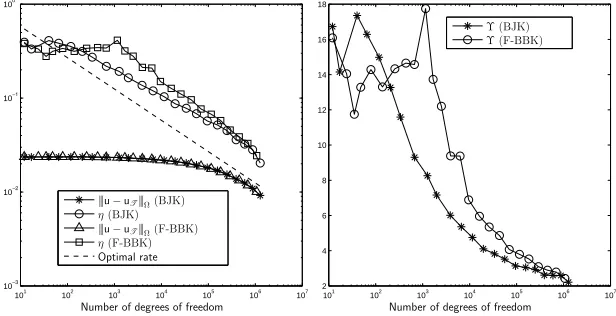
We report the results for this problem using the F-BBK method with C0 = 3 and p= 4, and the BJK method. From Figure9 we can see that the estimator and error follow a very similar pattern, and get closer as the mesh gets refined. This is confirmed on the right of Figure 9, where we depict the effectivity indices for this case. The initial mesh, and the approximate solution obtained after 23 steps of the adaptive scheme (which is, like the exact solution, non-negative), are depicted in Figure10.
Example 6 (A known three dimensional solution with a boundary layer). The
data for this example are as follows: ε= 10−3,b= (1,0,0)T,κ= 0,u
[image:17.612.100.415.94.476.2]100
101
102
103
104
105
106
107
10−3
10−2 10−1 100 101
Number of degrees of freedom
|||u−uT|||Ω,p= 4 η,p= 4
|||u−uT|||Ω,p= 6 η,p= 6
|||u−uT|||Ω,p= 8 η,p= 8 Optimal rate
100
101
102
103
104
105
106
107
10−3
10−2 10−1 100 101
Number of degrees of freedom
|||u−uT|||Ω,p= 4 η,p= 4
|||u−uT|||Ω,p= 6 η,p= 6
|||u−uT|||Ω,p= 8 η,p= 8 Optimal rate
Fig. 3. Example 1: The behaviour of the error |||u−uT|||Ω and estimator η, for the F-BBK
method, for uniform refinement (left) and adaptive refinement (right), for different values ofp.
0 0.1 0.2 0.3 0.4 0.5 0.6 0.7 0.8 0.9 1 0
0.05 0.1 0.15 0.2 0.25
x
uT(x,0.5) (p= 4) uT(x,0.5) (p= 6) uT(x,0.5) (p= 8)
u(x,0.5)
0.985 0.99 0.995 1
0.2435 0.244 0.2445 0.245 0.2455 0.246 0.2465 0.247 0.2475 0.248
x
uT(x,0.5) (p= 4)
uT(x,0.5) (p= 6) uT(x,0.5) (p= 8) u(x,0.5)
Fig. 4. Example 1: The 29th
adaptively refined meshes using the F-BBK method with p= 6
[image:18.612.75.431.77.280.2] [image:18.612.121.390.333.597.2]100
101
102
103
104
105
106
107
10−3
10−2
10−1 100
101
Number of degrees of freedom
η(BJK) η(F-BBK)
η(S-BBK)
Optimal rate
Fig. 5.Example2: Performance of the estimator.
right-hand side fis such that the exact solution is given by
(44) u(x, y, z) =yz(1−y)(1−z) x−e
−(1−x)
ε −e−
1
ε
1−e−1
ε
! .
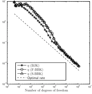
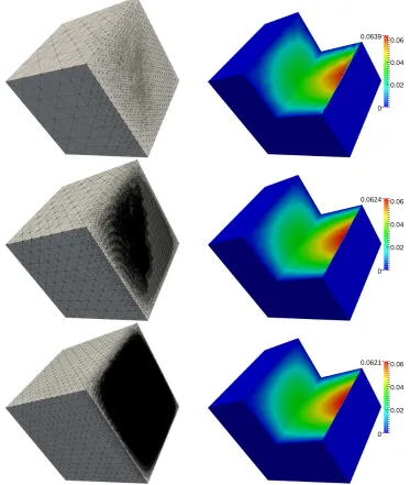
We report the results obtained using the F-BBK method with C0 = 3 and p= 10, and the BJK method, where the intial mesh is the same one as for the last example. In Figure 11 we depict the error and estimator, and effectivity indices. We can observe that the effectivity index does depend on the P´eclet number, but the error and estimator get to a good agreement once the mesh is refined enough. In Figure12 we depict the adapted meshes and the approximate solutions for different adaptive steps. We can observe that the mesh refinement is concentrated in the boundary layer region, and the solution respects the discrete maximum principle.
7. Concluding remarks. In this work we proposed and tested numerically a fully computable a posteriori error estimator for a shock-capturing like discretization of the convection-diffusion-reaction equation. The discretizations considered here are particular AFC schemes, but the presentation is general enough to accommodate any discretization that satisfies some basic hypotheses. More precisely, we have required the stabilization terms to be locally Lipschitz continuous, and locally linearity preserv-ing. These two assumptions have been previously used to prove optimal convergence. Interestingly, they were not needed to prove the fact that the estimator is a com-putable upper bound for the error, but they are essential for proving the local lower bounds. Future avenues of research include the study of robustness of the estima-tor with respect to ε, and the search for more effective ways to solve the resulting nonlinear system.
Acknowledgments. The authors would like to thank Diego Paredes and Petr Knobloch for many interesting discussions and suggestions.
REFERENCES
[1] M. Ainsworth, A. Allendes, G. R. Barrenechea, and R. Rankin, Fully computable a
[image:19.612.176.333.99.259.2]0.2 0.4 0.6
0 0.628
0.2 0.4 0.6
0 0.627
0.2 0.4 0.6
0 0.629
Fig. 6. Example2: The 30th
adaptively refined meshes and approximations obtained on these meshes, for the F-BBK method (top), S-BBK method (center) and BJK method (bottom).
problems in three dimensions, International Journal for Numerical Methods in Fluids, 73 (2013), pp. 765–790.
[2] M. Ainsworth and J. T. Oden,A posteriori error estimation in finite element analysis, Pure and Applied Mathematics (New York), Wiley-Interscience, New York, 2000.
[image:20.612.104.405.101.570.2]102
103
104
105
106
107
10−2
10−1
100 101
102
Number of degrees of freedom
η(F-BBK) η(BJK)
Optimal rate
0.25
0.5
0.75
0 1
0.25
0.5
0.75
0 1
Fig. 7.Example3: The evolution of the estimator through the mesh refinement process (top), and, for the full BBK method, the initial mesh and approximate solution on this mesh (center) and the mesh and approximate solution after 15 adaptive steps (bottom).
[4] P. R. Amestoy, I. S. Duff, J.-Y. L’Excellent, and J. Koster,A fully asynchronous multi-frontal solver using distributed dynamic scheduling, SIAM J. Matrix Anal. Appl., 23 (2001), pp. 15–41 (electronic).
[5] P. R. Amestoy, A. Guermouche, J.-Y. L’Excellent, and S. Pralet,Hybrid scheduling for
the parallel solution of linear systems, Parallel Comput., 32 (2006), pp. 136–156.
[6] R. Araya, A. H. Poza, and E. P. Stephan,A hierarchical a posteriori error estimate for
[image:21.612.101.402.95.551.2]102
103
104
105
106
107
10−3
10−2
10−1 100
101
Number of degrees of freedom
η(F-BBK) η(BJK)
Optimal rate
0 0.25 0.5 0.75
-9.05e-11 1
0 0.25 0.5 0.75
-3.14e-08 1
Fig. 8.Example4: The evolution of the estimator through the mesh refinement process (top), and, for the BJK method, the initial mesh and approximate solution on this mesh (center) and the mesh and approximate solution after 17 adaptive steps (bottom).
[7] S. Badia and A. Hierro,On monotonicity-preserving stabilized finite element approximations of transport problems, SIAM J. Sci. Comput., 36 (2014), pp. A2673–A2697.
[8] G. R. Barrenechea, E. Burman, and F. Karakatsani,Edge-based nonlinear diffusion for
finite element approximations of convection-diffusion equations and its relation to algebraic flux-correction schemes, Numer. Math., (to appear).
[image:22.612.97.385.95.581.2]satis-101 102 103 104 105 106 107 10−4
10−3
10−2
10−1
Number of degrees of freedom
|||u−uT|||Ω(F-BBK)
|||u−uT|||Ω(BJK)
η(F-BBK) η(BJK)
Optimal rate
101 102 103 104 105 106 107 1.8
2 2.2 2.4 2.6 2.8 3 3.2 3.4 3.6 3.8
Number of degrees of freedom Υ (F-BBK) Υ (BJK)
Fig. 9. Example 5: The behaviour of the error |||u−uT|||Ω and estimator η (left) and the
effectivity indicesΥ(right).
0.004 0.008 0.012
[image:23.612.99.411.103.264.2]0 0.0156
Fig. 10.Example5: Initial mesh (left) and the approximation obtained on the 23rd
adaptively refined mesh using the full BBK method (right).
101 102
103 104
105 106
107 10−3
10−2
10−1
100
Number of degrees of freedom
|||u−uT|||Ω(F-BBK)
|||u−uT|||Ω(BJK)
η(F-BBK) η(BJK)
Optimal rate
101 102
103 104
105 106
107 2
4 6 8 10 12 14 16 18
Number of degrees of freedom Υ (F-BBK) Υ (BJK)
Fig. 11. Example 6: The behaviour of the error|||u−uT|||Ω and estimator η (left) and the
[image:23.612.90.420.316.448.2] [image:23.612.101.409.498.656.2]0.02 0.04 0.06
0 0.0639
0.02 0.04 0.06
0 0.0624
0.02 0.04 0.06
[image:24.612.70.443.100.541.2]0 0.0621
Fig. 12.Example6: The 12th
(top), 17th
(center) and 22nd
(bottom) adaptively refined meshes (left) and approximate solutions (right) obtained on these meshes using the BJK method.
fying the discrete maximum principle and linearity preservation on general meshes, Necas Center for Mathematical Modeling preprint NCMM/2016/06, (2016).
[10] M. Bebendorf,A note on the Poincar´e inequality for convex domains, Z. Anal. Anwendungen, 22 (2003), pp. 751–756.
[11] S. Berrone,Robustness in a posteriori error analysis for FEM flow models, Numer. Math., 91 (2002), pp. 389–422.
[13] E. Burman and A. Ern,Nonlinear diffusion and discrete maximum principle for stabilized Galerkin approximations of the convection–diffusion-reaction equation, Comput. Methods Appl. Mech. Engrg., 191 (2002), pp. 3833–3855.
[14] E. Burman and A. Ern,Stabilized Galerkin approximation of convection–diffusion–reaction equations: discrete maximum principle and convergence, Math. Comp., 74 (2005), pp. 1637–1652.
[15] P. G. Ciarlet,The finite element method for elliptic problems, SIAM, Philadelphia, PA, 2002.
[16] B. Cockburn and P.-A. Gremaud, Error estimates for finite element methods for scalar
conservation laws, SIAM J. Numer. Anal., 33 (1996), pp. 522–554.
[17] K. Eriksson and C. Johnson,Adaptive streamline diffusion finite element methods for sta-tionary convection-diffusion problems, Math. Comp., 60 (1993), pp. 167–188, S1–S2. [18] A. Ern and J.-L. Guermond,Theory and practice of finite elements, vol. 159, Springer Science
& Business Media, 2013.
[19] A. Ern and J.-L. Guermond,Weighting the edge stabilization, SIAM J. Numer. Anal., 51
(2013), pp. 1655–1677.
[20] A. Ern, A. F. Stephansen, and M. Vohral´ık,Guaranteed and robust discontinuous Galerkin a posteriori error estimates for convection-diffusion-reaction problems, J. Comput. Appl. Math., 234 (2010), pp. 114–130.
[21] S. K. Godunov,A difference method for numerical calculation of discontinuous solutions of the equations of hydrodynamics, Mat. Sb. (N.S.), 47 (89) (1959), pp. 271–306.
[22] P. Grisvard,Elliptic problems in nonsmooth domains, vol. 69 of Classics in Applied Mathe-matics, Society for Industrial and Applied Mathematics (SIAM), Philadelphia, PA, 2011. Reprint of the 1985 original [ MR0775683], With a foreword by Susanne C. Brenner.
[23] V. John and P. Knobloch,On spurious oscillations at layers diminishing (SOLD) methods
for convection–diffusion equations: Part I – A review, Comput. Methods Appl. Mech. En-grg., 196 (2007), pp. 2197–2215.
[24] V. John and P. Knobloch,On spurious oscillations at layers diminishing (SOLD) methods
for convection–diffusion equations: Part II – Analysis for P1 and Q1 finite elements,
Comput. Methods Appl. Mech. Engrg., 197 (2008), pp. 1997–2014.
[25] V. John and J. Novo, A robust SUPG norm a posteriori error estimator for stationary
convection-diffusion equations, Comput. Methods Appl. Mech. Engrg., 255 (2013), pp. 289– 305.
[26] T. Knopp, G. Lube, and G. Rapin,Stabilized finite element methods with shock capturing for advection-diffusion problems, Comput. Methods Appl. Mech. Engrg., 191 (2002), pp. 2997– 3013.
[27] D. Kuzmin,Algebraic flux correction for finite element discretizations of coupled systems, in Proceedings of the Int. Conf. on Computational Methods for Coupled Problems in Science and Engineering, M. Papadrakakis, E. O˜nate, and B. Schrefler, eds., CIMNE, Barcelona, 2007, pp. 1–5.
[28] D. Kuzmin and M. M¨oller,Algebraic flux correction. I. Scalar conservation laws, in Flux-corrected transport, Sci. Comput., Springer, Berlin, 2005, pp. 155–206.
[29] D. Kuzmin, M. M¨oller, and S. Turek,High-resolution FEM-FCT schemes for
multidimen-sional conservation laws, Comput. Methods Appl. Mech. Engrg., 193 (2004), pp. 4915– 4946.
[30] D. Kuzmin and J. N. Shadid,A new approach to enforcing discrete maximum principles in
continuous Galerkin methods for convection-dominated transport equations, tech. report, UA Ruhr Zentrum f¨ur partielle Differentialgleichungen, 2015.
[31] MATLAB,(R2013a), The MathWorks Inc., Natick, Massachusetts, 2013.
[32] A. Mizukami and T. J. R. Hughes,A Petrov-Galerkin finite element method for convection-dominated flows: an accurate upwinding technique for satisfying the maximum principle, Comput. Methods Appl. Mech. Engrg., 50 (1985), pp. 181–193.
[33] L. E. Payne and H. F. Weinberger,An optimal Poincar´e inequality for convex domains,
Arch. Rational Mech. Anal., 5 (1960), pp. 286–292 (1960).
[34] G. Sangalli,Robust a-posteriori estimator for advection-diffusion-reaction problems, Math. Comp., 77 (2008), pp. 41–70.
[35] L. Tobiska and R. Verf¨urth,Robust a posteriori error estimates for stabilized finite element methods, IMA J. Numer. Anal., 35 (2015), pp. 1652–1671.
[36] R. Verf¨urth,A review of a posteriori error estimation and adaptive mesh-refinement tech-niques, John Wiley & Sons Inc, 1996.
[37] R. Verf¨urth,A posteriori error estimators for convection-diffusion equations, Numer. Math., 80 (1998), pp. 641–663.
equa-tions, SIAM J. Numer. Anal., 43 (2005), pp. 1783–1802 (electronic).
[39] J. Xu and L. Zikatanov,A monotone finite element scheme for convection-diffusion equa-tions, Math. Comp, 68 (1999), pp. 1429–1446.