City, University of London Institutional Repository
Citation
:
Morgan, M. J., Giora, E. and Solomon, J. A. (2008). A single "stopwatch" for duration estimation, A single "ruler" for size. Journal of Vision, 8(2), .14. doi: 10.1167/8.2.14This is the published version of the paper.
This version of the publication may differ from the final published
version.
Permanent repository link:
http://openaccess.city.ac.uk/14913/Link to published version
:
http://dx.doi.org/10.1167/8.2.14Copyright and reuse:
City Research Online aims to make research
outputs of City, University of London available to a wider audience.
Copyright and Moral Rights remain with the author(s) and/or copyright
holders. URLs from City Research Online may be freely distributed and
linked to.
A single
“
stopwatch
”
for duration estimation,
A single
“
ruler
”
for size
Department of Optometry and Visual Science, City University, London, UK
Michael J.
Morgan
Dipartimento di Psicologia Generale, Università di Padova, Padova, Italy
Enrico
Giora
Department of Optometry and Visual Science, City University, London, UK
Joshua A.
Solomon
Although observers can discriminate visual targets with long exposures from otherwise-identical targets with shorter exposures, temporally overlapping distracters with an intermediate exposure can produce a striking degradation in performance. This newfinding suggests that observers can only estimate one duration at a time. Discrimination on the basis of size, rather than duration, did not degrade as rapidly with the number of distracters but was still worse than predicted by unlimited-capacity models. The critical difference between estimates of temporal length and estimates of spatial length seems to be that the former can only be made at the end of an exposure, while the latter can be made at any time during an exposure. When sizes varied throughout the trial and decisions were based on terminal sizes, the set-size effect was as large as that obtained for duration discrimination. We conclude that when texturalfilters are not available for segregating a target from distracters, efficient estimates of size or duration require the serial examination of individual display items. Keywords: timing, search efficiency, averaging, signal detection theory
Citation:Morgan, M. J., Giora, E., & Solomon, J. A. (2008). A single“stopwatch”for duration estimation: A single“ruler”for size.Journal of Vision, 8(2):14, 1–8, http://journalofvision.org/8/2/14/, doi:10.1167/8.2.14.
Introduction
The conception of space and time as a four-dimensional manifold has been fruitful for mathematical physics. However, the treatment of space and time as a manifold does not mean that time is just another spatial dimension (Reichenbach,1958). The special properties of time, such as its uni-directionality, are not necessarily affected by making it one axis of a manifold, any more than pitch is made into a spatial dimension by a sound spectrograph. Granting Reichenbach’s (1958) point, it is still fruitful to explore the formal analogies between space and time by the experimental method. Such analogies have proved useful in psychophysics as well as in physics. For example, the idea of applying Fourier analysis to contrast sensitivity in space–space axes (Campbell & Robson, 1968) was foreshadowed by De Lange’s (1952) equivalent analysis of temporal sensitivity in space–time. Equally interesting insights into motion processing have been gained by Fourier transforms in the space–time manifold (Adelson & Bergen, 1985; Morgan, 1980; Ross & Burr, 1983; Watson & Ahumada, 1985).
In this paper, we explore the formal analogy between space and time using a visual search paradigm. Consider the events shown in Figure 1. If the two axes were
considered as space–space (x, y), the search items would be lines, all having the same length except one, which is shorter. An observer could search for this “odd line out” and decide whether it was shorter or longer than the others. Palmer, Ames, and Lindsey (1993) used a related procedure and found that the number of line segments did not affect the precision with which odd-lines-out were detected. One interpretation of this unlimited capacity for simultaneous length estimates is that observers have access to multiple “rulers” (i.e., visual analyzers capable of estimating size) distributed over space. Alternative interpretations will be considered below.
items. In other words, a large set-size effect may indicate that there is only a single master clock, whichVlike a stopwatchVrequires the observer’s attention to start and read.
We tested these predictions in a visual search task where the target differed from multiple distracters either in size or in duration. The stimuli in the two tasks were identical except for the size or the duration cue (see Methods). As the target length increased (in either time or space), so did the proportion of “longer” responses. “Threshold” lengths, that is, those required for consistent responses, were derived from the (psychometric) functions mapping target length to the proportion of “longer” responses (see Methods). In order to compare perfor-mance in space and time, perforperfor-mances were expressed as dimensionless Weber fractions (threshold/standard;$L/L).
Methods
A practical limitation made it impossible to carry out the experiment in exactly the manner illustrated in the two-dimensional manifold ofFigure 1. A visual stimulus, even if it is notionally a point, must be two-dimensional, and it must have a duration. Therefore, both the temporal and the spatial tasks must have three dimensions (two of space and one of time). Given this limitation, we decided to make the spatial arrays identical in the spatial and the temporal tasks. The events consisted of lines (or in some experiments, circles) staggered in space as inFigure 1. For symmetry, the events in both tasks were staggered in time, as shown in Figure 1. The “medium” (i.e., 2.0 s; see below) duration was used in the spatial tasks and the medium (i.e., 5.0 cm) size was used in the temporal tasks. Only one kind of difference, spatial or temporal, was present in any block of trials.
Stimuli
Displays were generated on a Sony Trinitron VDU under the control of a Cambridge Research Systems VSG2/5 graphics processor and MATLAB software. The display was viewed in a room with normal fluorescent lighting. Viewing distance (2 m) was such that 1 cm on the screen subtended 0.3-. In experiments where lines were the stimuli, the lines were horizontal and had random horizontal offsets in the range 0 G x G s,
where s was the standard length in the experiment. In Experiment 1, the lines were presented in a random temporal order, with random temporal offsets from the start of the trial. InExperiment 2, the stimuli were circles, and the circles were arranged at equal intervals around an iso-eccentric circle of diameter 10-. The temporal offsets were staggered rather than random, such that each stimulus appeared at a random time during the preceding stimulus.
Psychophysics
The observer’s task on each trial was to press one of two buttons to indicate whether the target was longer or shorter than the standard (in time or in space). Correct responses were followed by a brief, bright flash. The timing and spatial tasks were presented in separate sessions, but within each session, the four different set sizes were randomly interleaved. Each session lasted for 256 (464) trials. The observer’s psychometric function was sampled by the APE procedure (Watt & Andrews, 1981). Threshold was defined as the standard deviation of the best-fitting cumulative Gaussian to the psychometric function, which corresponds to 82.9% correct in the absence of bias. Biases were derived from the means of the best-fitting Gaussians but were not further analyzed.
Modeling
We fit the Max rule of signal detection theory (see below) to experiments requiring a “long” or a “short” response. The same model was used for both spatial and temporal judgments. Prior to fitting the Max rule, each psychometric function mapping target length to the frequency of a “long” response was maximum-likelihood fit with a two-parameter Gaussian distribution (C.D.F.) The mean of this distribution was then subtracted from stimulus length, allowing us to fit an unbiased Max rule to individual responses (rather than just thresholds), which were guaranteed to be free of bias. NB: After this bias correction, the standard length for any unbiased observer is zero.
[image:3.612.68.262.60.219.2]In accordance with signal detection theory (Green & Swets, 1966), our modeling assumes that the apparent
Figure 1. Space–time diagram of the stimuli used in the experiments.
length of each distracter can be described with an independent zero-mean Gaussian random variable. Let
fD(u) and FD(u) denote its density (P.D.F.) and distribu-tion, respectively. We assume that the apparent length of the target has the same variance A2 but has a non-zero mean 2, equal to the difference between target and distracter lengths. Let fT(u; 2) and FT(u; 2) denote its density and distribution, respectively.
According to the Max rule, the probability of a “long” response is given by
p2¼
Z V
0
fTðu;2Þ½FDð Þju FDðjuÞ
M
þMfDð Þu ½FTðu;2ÞjFTðju;2Þ ½FDð Þju FDðjuÞ
Mj1du;
whereMis the number of distracters (Morgan & Solomon, 2005).
In general, variance was allowed to increase with set size, such that A = aM + A1. Values for a and A1
were found that maximized the log-likelihood of all responses
L¼ln P2þQ2
P2
þP2lnp2þQ2ln 1j p2; ð2Þ
where P2 and Q2 denote the number of “long” and “short” responses, respectively, that were collected when the difference between target and distracter lengths was2.
Results
Experiment 1
The first experiment measured thresholds for set sizes
[image:4.612.127.491.360.666.2]M = 1, 2, 4, and 8 at short, medium, and long standard temporal durations (0.5, 2.0, and 8.0 s). The spatial standards were 1.25, 5.0, and 20.0 cm. In the temporal task, the spatial length was always 5.0 cm, and in the
Figure 2.Results for two observers (EG and FG) inExperiment 1. Red symbols show threshold Weber fractions (vertical axis) in the temporal task, and black symbols show thresholds for the spatial task. Each panel shows the data for a single observer under one of the three baseline conditions (small, medium, and large standards). The colored lines showfits of the increasing-noise version of the Max model (red for temporal and black for spatial task) compared tofits of the averaging model (green for temporal and blue for spatial task). For explanation of the models, see text.
spatial task, the temporal duration was 2.0 s. The observers were one of the authors (EG) and a psycho-physically naive young male observer FG, who was not informed of the purpose of the experiment. Additional observations were carried out using the medium standard duration by MM and by another psychophysically naive young male (SG).
Maximum-likelihood estimates of threshold Weber fractions (see Methods) appear in Figure 2. It appears fromFigure 2that the temporal task is more difficult than the spatial task. Before concluding that the temporal task is harder than the spatial, a possible problem to be considered is that there is no natural metric for comparing the spatial and the temporal standards. A “short” length might correspond in its internal representation to a “long” duration. If Weber fractions were constant, as Weber’s Law claims, this would not matter. To test for significant differences between Weber fractions, we used only the
M= 1 data and fit the short, medium, and long conditions separately, with two-parameter psychometric functions of Weber fraction. The joint likelihood,LU, of these uncon-strained fits was compared with the joint likelihood,LC, of fits in which the threshold parameter was constrained to be identical in all three conditions. The “generalized” ratio of these likelihoods j2ln(LC/LU), can then be compared to
the chi-square distribution with 2 degrees of freedom (because the constrained fit has 2 fewer free parameters; Mood, Graybill, & Boes,1974).
Applying this chi-square test to our spatial data, we found the generalized likelihood ratios to be 0.1 for EG and 4.3 for FG, whereas the critical value#0.952(2) = 6.0. Thus, the separate fits were not significantly different, and we have no evidence against Weber’s Law. However, the same test of our temporal data tells a different story. The generalized likelihood ratios were 58 for EG and 14 for FG. Thus, the separate fits were significantly different, and Weber’s Law did not hold for duration. Therefore, some temporal standards may be remembered with relatively greater precision than others. The Weber fraction for comparison with these “easy” durations may be compara-ble to that for size comparisons.
In some conditions (e.g., “medium”), the relative difficulty of the temporal task appeared to increase with set size. However, there was a set size effect for both tasks. A small set-size effect in spatial tasks has been reported before (Palmer et al.,1993; Treisman,1988) and is not necessarily inconsistent with unlimited capacity once the effects of spatial uncertainty have been taken into account. If an “early” source of perceptual noise perturbed each estimate of spatial and temporal length, then the total amount of noise would increase with set size. One possible strategy would be to select the (noisy) estimate that has the greatest absolute difference from the standard and to report the sign of that difference. This “Max rule” of signal detection theory has provided a successful description of many set-size effects (Morgan & Solomon, 2005).
We fit the data in Figure 2 with the Max model and found that the fit was poor. (Fitted values of internal noise and log-likelihoods are documented in Table 1.) Thresh-olds rose more rapidly with set size than predicted by the Max rule. To quantify how much bigger than the Max model’s prediction our set-size effects were, we consid-ered a modification of the Max model, in which there was a linear relationship between the number of search items and the standard deviation of the perceptual noise. Maximum-likelihood fits of this model are shown in
Figure 2 and in Table 1. The addition of the second
parameter improved the fit over the Max model signifi-cantly in every case, except for FG in the “short” temporal condition. (Specifically, with the one exception, the generalized likelihood ratio of the two fits exceeded the critical value #0.99992(1) = 15.1; see Table 1.) In general, the precision of temporal estimates fell more rapidly with set size than the precision of spatial estimates. Spatial noise increased less than 1% with each additional item, butVwith the exception of FG in the “short” condi-tionVtemporal noise increased more than 1% with each additional search item.
We also considered an averaging model of performance, in which the observer computes on each trial the mean value over all the stimuli (Morgan, Ward, & Castet,1998; Parkes, Lund, Angelucci, Solomon, & Morgan,2001) and compares it to the standard. The averaging model was a poorer fit than the two-parameter increasing-noise version of the Max model in all cases except FG in the short/ temporal condition. The fit of the unmodified Max model was better than that of the averaging model in all cases (Table 1).
Several panels in Figure 2 show a large increase in duration thresholds when the number of items increases from 1 to 2. This suggests that we cannot accurately assess the duration of two temporally overlapping events. Of course, having a single stopwatch does not preclude multiple duration estimates in a single trial; it merely precludes parallel estimates. Very long targets can always be at least partially monitored because they will be the last to disappear. Even a single stopwatch can tell when the duration between the last two disappearances is much longer than the standard. Therefore, psychometric func-tions should always have ceilings near 100%.
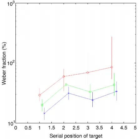
Observer EG reported that he based several decisions on the first search item to be presented. To investigate this point, further data were collected. These new data (shown
in Figure 3) confirmed that accuracy was indeed highest
when the target was presented first. EG also reported using the temporal order of onset and offset as a cue. Suppose four items numbered 1–4 appear in the temporal order [4 1 3 2] and disappear in the order [1 3 2 4]. It is clear that item 4 is longer than the other. Similarly, the onset pattern [1 4 2 3] followed by [4 1 2 3] means that item 4 is shorter than the others. This is not a high precision strategy since it is unavailable in the case [4 1 3 2] followed by offsets [4 1 3 2].
The highly inefficient search for duration is compatible with two explanations. The first is that there is only a single master stopwatch, which can estimate only one duration at a time. The second is that there are multiple stopwatches distributed around the visual field, butVunlike real stopwatchesVthey have to be read soon after they have
been stopped. According to the latter interpretation, the reason for the inefficiency with overlapping durations is that while the observer is reading one stopwatch, another may terminate and lose its information before the observer can read it. These two interpretations would be difficult to distinguish experimentally.
A1for
time (%)
A1for
space (%)
!for time (%/M)
!for space (%/M)
jLfor time
jLfor space
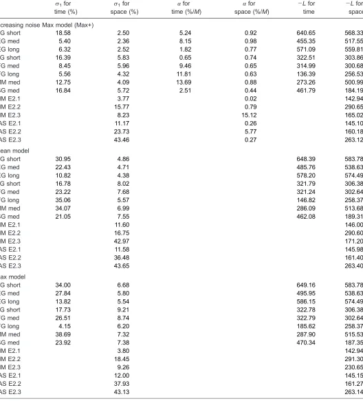
Increasing noise Max model (Max+)
EG short 18.58 2.50 5.24 0.92 640.65 568.33 EG med 5.40 2.36 8.15 0.98 455.35 517.55 EG long 6.32 2.52 1.82 0.77 571.09 559.81 FG short 16.39 5.83 0.65 0.74 322.51 303.86 FG med 8.45 5.96 9.46 0.65 314.99 300.68 FG long 5.56 4.32 11.81 0.63 136.39 256.53 MM med 12.75 4.09 13.69 0.88 273.26 500.99 SG med 16.84 5.72 2.51 0.44 461.79 184.19
MM E2.1 3.77 0.02 142.94
MM E2.2 15.77 0.79 290.65
MM E2.3 8.23 15.12 165.02
JAS E2.1 11.17 0.26 145.10
JAS E2.2 23.73 5.77 160.18
JAS E2.3 43.46 0.27 263.12
Mean model
EG short 30.95 4.86 648.39 583.78
EG med 22.43 4.71 485.76 538.63
EG long 10.82 4.38 578.20 574.49
FG short 16.78 8.02 321.79 306.38
FG med 23.22 7.68 321.24 302.64
FG long 35.06 5.57 146.82 258.37
MM med 34.07 6.99 286.09 513.68
SG med 21.05 7.55 462.08 189.31
MM E2.1 11.60 146.00
MM E2.2 16.75 290.60
MM E2.3 42.97 171.20
JAS E2.1 11.58 145.98
JAS E2.2 36.48 161.40
JAS E2.3 43.65 263.40
Max model
EG short 34.00 6.68 649.16 583.78
EG med 27.84 5.80 495.95 538.63
EG long 13.82 5.54 586.15 574.49
FG short 17.73 9.21 322.78 306.38
FG med 26.51 8.74 322.79 302.64
FG long 4.15 6.20 185.62 258.37
MM med 38.69 7.32 287.90 515.53
SG med 23.92 7.38 470.34 187.35
MM E2.1 3.80 142.94
MM E2.2 18.45 291.30
MM E2.3 9.26 230.65
JAS E2.1 12.00 145.15
JAS E2.2 37.93 161.27
[image:6.612.44.572.59.642.2]JAS E2.3 43.13 263.14
The greater efficiency of search for size may suggest that there are multiple “rulers” distributed over space, but it is not inconsistent with the notion of a single ruler. Whereas duration information only becomes available at the end of an event, size information remains available throughout. This reasoning suggests that it might be
possible to devise a size task with a capacity limit similar to that for the duration task. This could be done by making the size information available for only a brief moment at the end of the stimulus. This was the aim of our second experiment.
Experiment 2
In this experiment, there were three different tasks. In the simple spatial control task (E2.1), each stimulus had a constant size during its presentation. In the “grow” task (E2.2), each item appeared as a point and expanded in size until it reached the standard size, at which time it disappeared. The target’s terminal size was slightly larger or smaller than the standard. In the “grow–shrink” task (E2.3), the stimuli appeared at random sizes in the range 0 G xG 2s,wheres was the standard, and grew orshrank
until all but one reached the standard size.
[image:7.612.56.278.59.281.2]The results (Figure 4andTable 1) showed that the two “growth” tasks were much harder than the simple size task. Data for the simple size task were well fit by the Max model. In fact, the Max+ model made no significant improvement (Table 1), unlike the findings of the first experiment. This could have been because of the shape of the stimuli (circles vs. lines), or more likely because the staggered presentation was easier than the random. Base-line thresholds when there were no distracters were higher in both of the “growth” conditions than in the simple size task for both observers. The effects of set size were less clear. Only in one case (MM grow–shrink) was the Max+ model a significantly better fit than the Max. However, it is clear from Figure 4that performance was worse in the “grow” conditions than in the simple size task at all set sizes and for both observers.
Figure 4. The figure shows thresholds (vertical axis) for size discrimination (black symbols and lines) as a function of set size in
[image:7.612.139.474.495.666.2]Experiment 2. Two other conditions are also shown. In the“grow”version (red symbols and lines), the stimuli started as points and grew to their terminal size. In the“grow–shrink”version (blue symbols and size), the stimuli started at a random size and then either grew or shrank to their terminal size. Thefits show a version of the MAX model in which noise increases linearly with set size (seeTable 1and text).
Figure 3. Temporal thresholds for one observer (EG) from
Experiment 1, plotted separately according to the temporal position (horizontal axis) of the target in the sequence. The three curves show the data separately for short (red circles; 0.5 s), medium (green squares; 2 s), and long (blue stars; 8 s) standard intervals, respectively. The data for the three conditions have been displaced on the horizontal axis for clarity.
We conclude from these results that there are severe limitations for both duration and size tasks, provided the observer is prevented in the latter from having sufficient time to inspect each of the targets.
Discussion
The results of our Experiment 2 suggest that search for size can have the same severe capacity limit as the search for duration, provided that the stimuli are presented sufficiently briefly to prevent serial inspection. At first sight, this conclusion seems to contradict the finding by Palmer et al. (1993) of highly efficient search for size, using displays presented for only 100 ms. (Observers had to decide which of every pair of displays contained a target that was longer than the distracters.) However, we do not know how many shifts of attention are possible in 100 ms. Palmer et al. used a maximum of 8 stimuli per display, and it is possible that a capacity limit for a brief display would appear with a greater number of distracters. Another point is that Palmer et al. did not use a postmask, so the actual time available to the observer for inspecting iconic memory might have been considerably longer than 100 ms (Sperling,1960). When a postmask is used, there is a severe capacity limit for orientation search (Baldassi & Burr,2000; Morgan & Solomon,2005; Morgan et al.,
1998; Solomon & Morgan, 2001), and the same may be
true for size, although this has not been directly demonstrated. Morgan et al. (1998) showed that as the exposure duration of a postmasked display was increased, performance approximated more and more closely to those reported by Palmer et al. for size, viz., unlimited capacity. We therefore think that the jury must stay out on the question whether there is strictly unlimited capacity for size search when serial inspection is prevented. Therefore, there may be a single ruler for size, just as there seems to be a single stopwatch for duration.
The simplest explanation for our data is that there is a single “stopwatch” for durations and a single “ruler” for sizes. Our results may seem to be inconsistent with those recently cited as evidence against a “single universal clock” (Johnston et al., 2006), but we believe they are not. Johnston et al. (2006) showed that adaptation to a periodic (either oscillating or flickering) stimulus affected the apparent duration of a subsequent stimulus only when it appeared at the same position. They concluded that there were independently adaptable, localized mecha-nisms for duration estimation. Within the context of that conclusion, our results imply that focal attention is required to “read” the output of any of these mechanisms one at a time.
On the other hand, we would also like to note that Johnston et al.’s (2006) finding is not incompatible with the notion of a single stopwatch. Previous research has
shown that periodic stimuli typically appear to last longer than static stimuli (Refs. 25 and 26 from Johnston et al., 2006). Johnston et al.’s finding suggests that the influence of periodicity on duration estimation may be reduced following adaptation to another, appropriately positioned, periodic stimulus. Johnston et al. seem to suggest some-thing like this when they say that the local signals are scaled. Therefore, their data are compatible with a single, central duration estimator that collects various forms of evidence from a stimulus and perhaps even combines them in a Bayesian manner. Since the difference between this idea and that of separate mechanisms requiring attentive access is largely semantic, we believe that it is premature to discard the intuitively appealing idea of a single, central, stopwatch for duration estimation.
Acknowledgments
This work was supported by a grant from The Wellcome Trust.
Commercial relationships: none.
Corresponding author: Joshua A. Solomon. Email: [email protected].
Address: Department of Optometry and Visual Science, City University, London, EC1V 0HB, UK.
References
Adelson, E. H., & Bergen, J. R. (1985). Spatiotemporal energy models for the perception of motion.Journal of the Optical Society of America A, Optics and Image Science, 2,284–299. [PubMed]
Baldassi, S., & Burr, D. C. (2000). Feature-based integration of orientation signals in visual search.
Vision Research, 40,1293–1300. [PubMed]
Campbell, F. W., & Robson, J. G. (1968). Application of Fourier analysis to the visibility of gratings. The Journal of Physiology, 197, 551–566. [PubMed] [Article]
De Lange, H. (1952). Experiments on flicker and some calculations on an electrical analogue of the foveal systems.Physica, 18, 935–950.
Green, D. M., & Swets, J. A. (1966). Signal detection theory and psychophysics. New York: Wiley.
Johnston, A., Arnold, D. H., & Nishida, S. (2006). Spatially localized distortions of event time. Current Biology, 16, 472–479. [PubMed] [Article]
Mood, A. M., Graybill, F. A., & Boes, D. C. (1974).
Morgan, M. J. (1980). Analogue models of motion perception.Philosophical Transactions of the Royal Society of London B: Biological Sciences, 290,
117–135. [PubMed]
Morgan, M. J., & Solomon, J. A. (2005). Capacity limits for Spatial Discrimination. In L. Itti, G. Rees, & J. Tsotsos (Eds.), Neurobiology of Attention. San Diego, CA: Elsevier.
Morgan, M. J., Ward, R. M., & Castet, E. (1998). Visual search for a tilted target: Tests of the spatial uncertainty model.Quarterly Journal of Experimental Psychology A: Human Experimental Psychology, 51,
347–370. [PubMed]
Palmer, J., Ames, C. T., & Lindsey, D. T. (1993). Measuring the effect of attention on simple visual search. Journal of Experimental Psychology: Human Perception and Performance, 19,108–130. [PubMed] Parkes, L., Lund, J., Angelucci, A., Solomon, J. A., & Morgan, M. J. (2001). Compulsory averaging of crowded orientation signals in human vision. Nature Neuroscience, 4, 739–744. [PubMed] [Article] Reichenbach, H. (1958). The philosophy of space and
time. New York: Dover.
Ross, J., & Burr, D. (1983). The psychophysics of motion. In M. Arbib, & A. R. Hanson (Eds.), Vision, brain and cooperative processes. Amherst, MA: Bradford. Solomon, J. A., & Morgan, M. J. (2001). Odd-men-out are
poorly localised in brief exposuresJournal of Vision, 1(1):2, 9–17, http://journalofvision.org/1/1/2/, doi:10.1167/1.1.2. [PubMed] [Article]
Sperling, G. (1960). The information available in brief visual presentations. Psychological Monographs: General and Applied, 74,1–30.
Treisman, A. (1988). Features and objects: The fourteenth Bartlett memorial lecture. Quarterly Journal of Experimental Psychology A: Human Experimental Psychology, 40,201–237. [PubMed]
Watson, A. B., & Ahumada, A. J., Jr. (1985). Model of human visual-motion sensing. Journal of the Optical Society of America A Optics and Image Science, 2,
322–341. [PubMed]
Watt, R. J., & Andrews, D. P. (1981). APE: Adaptive probit estimation of a psychometric function.Current Psychological Reviews, 1,205–214.