Operation Efficiency Optimisation Modelling and
Application of Model Predictive Control
Xiaohua Xia and Jiangfeng Zhang
Abstract—The efficiency of any energy system can be chara-terised by the relevant efficiency components in terms of perfor-mance, operation, equipment and technology (POET). The over-all energy efficiency of the system can be optimised by studying the POET energy efficiency components. For an existing energy system, the improvement of operation efficiency will usually be a quick win for energy efficiency. Therefore, operation efficiency improvement will be the main purpose of this paper. General procedures to establish operation efficiency optimisation models are presented. Model predictive control, a popular technique in modern control theory, is applied to solve the obtained energy models. From the case studies in water pumping systems, model predictive control will have a prosperous application in more energy efficiency problems.
Index Terms—Model predictive control (MPC), operation effi-ciency, energy efficiency.
I. INTRODUCTION
W
ITH the increasing shortage of energy supply, energy efficiency improvement has been widely recognised as the quickest and most effective method to alleviate en-ergy supply pressure. Enen-ergy efficiency generally consists of many components, such as management efficiency, oper-ational efficiency, carrier efficiency, information and control efficiency, billing efficiency, maintenance efficiency, conver-sion efficiency, thermal efficiency, luminous efficiency, etc. In [1−3], these energy efficiency components were summarised and classified as performance efficiency, operation efficiency, equipment efficiency, and technology efficiency (POET). A prominent application of this kind of POET classification is to prevent the loss of energy efficiency improvement opportu-nities, which is shown in the energy audit practices[4]. This POET classification can also be applied to general energy optimisation so that all the key aspects of energy efficiency are optimised. Note the fact that proper sizing and matching of different system components, which include changing the operational schedules amongst others, for a given energy system will often save both energy and energy cost in many scenarios, therefore this paper focuses on the operation effi-ciency optimisation. Operation effieffi-ciency is often evaluated in terms of performance indicators such as energy, power, cost, etc.[1]. It follows that operation efficiency can usually beThis work was supported by National Research Foundation of South Africa (UID85783), the National Hub for Energy Efficiency and Demand Side Management and Exxaro.
Xiaohua Xia is with the Department of Electrical, Electronic and Computer Engineering, University of Pretoria, Pretoria 0002, South Africa (e-mail: [email protected]).
Jiangfeng Zhang is with the Department of Electronic and Elec-trical Engineering, University of Strathclyde, G1 1XW, UK (e-mail: [email protected]).
written as an optimisation problem with objective functions to be the minimisation of energy or power consumption, energy cost, etc. This kind of optimisation problem is formulated over a given time period, and can often be understood as an optimal control problem since the time dependent operation functions can be treated as the control input in optimal control. Thus various control techniques will be applicable to these energy problems. This paper focuses on the establishment of operation efficiency optimisation models and the application of model predictive control (MPC) to solve the obtained models.
MPC is well-known for its ability to use simple models, to handle constraints, and also for its closed-loop stability and inherent robustness. Therefore, MPC has become a popular tool for many industrial problems[5−7]. The MPC technique can be applied to many operation efficiency optimisation problems in which the energy systems are operated over evolving time spans. In the literature, there are various case studies on operation efficiency optimisation, and these studies include cases such as steel plant peak load management[8], energy management of a petrochemical plant[9], rock winder systems[10], water pumping systems[11−12], power generation economic dispatch[13], power generation maintenance[14], etc. From these studies, it turns out that the most challenging part in the MPC applications is not the MPC itself, but the energy system modelling. Also existing studies focus on particular systems only, a general description on the operation efficiency optimisation modelling techniques is necessary. This paper summarises these modelling techniques and particularly formulates the general logic correlation constraints. These general modelling principles are illustrated by a few examples which include mineral processing, pumping systems and plant maintenance.
The paper is organized as follows. The next section pro-vides a unified modelling framework for operation efficiency optimisation. General steps to apply MPC principles are also summarised. Section III provides some case studies, and the last section is the conclusion.
II. OPERATION EFFICIENCY OPTIMISATION MODELLING ANDMPCAPPLICATIONS
coordination parts. Operation efficiency has the following indicators: physical coordination indicators (sizing and match-ing); time coordination indicator (time control); and human coordination indicator. It is usually difficult to model the human coordinations in operation efficiency, therefore we will focus on the physical and time coordination indicators.
A. Optimal Control Modelling for Operation Efficiency
The purpose to optimise operation efficiency is usually to save energy and energy cost while at the same time to meet certain service requirement. In the following, the objec-tive functions of the operation efficiency operation model will be chosen as both the energy and energy cost.
Assume that an energy system consists of N components, each of them can be independently controlled as on or off. Whenever the i-th component is switched on, its power con-sumption will be its rated powerPikW fori= 1,2,· · ·, N1, and be any value between 0 and its rated power Pi kW for
i = N1 + 1, N2 + 2,· · ·, N, where N1 ≤ N. The first N1 components have only simple on/off status and include examples such as electric water heaters, electric kettles, and incandescent lights, while the last N−N1 components have variant powers and examples can be motors controlled by variable speed drives. Let the energy price at time tbe $p(t)/ kWh; then the energy consumption function fE and energy
cost function fC over a fixed time interval [t0, tf] are given
below.
fE=
Z tf
t0
N
X
i=1
Piui(t)dt,
fC=
Z tf
t0
N
X
i=1
Piui(t)p(t)dt, (1)
whereui(t)represents the on/off status variable and is defined
as follows:
ui(t)
= 1,if thei-th component is on and 1≤i≤N1
= 0,if thei-th component is off and1≤i≤N1 ∈[0,1], ifN1≤i≤N
The two functions fE and fC will be minimised. After
formulating these two objective functions, the remaining part on the modelling is to find proper constraints. The coordi-nation within the N components of the system can be very complicated. For illustration purposes, the following typical types of coordination relations between these N components are modelled.
1) Logic correlations
a) The statusui(ta)does not affect the status ofuj(tb). For
this case, we do not need to build any mathematical constraint. b) If ui(ta) is in the switched on status, thenuj(tb) must
be in the off status. To find out a mathematical equivalent expression for this constraint, the following sign function is introduced. Let sgn(x) be 1 ifx >0; 0 if x= 0; and −1 if x <0. Noting the fact thatui(ta)anduj(tb)are nonnegative,
then it follows that this constraint is equivalent to:
(sgn(ui(ta)) + 1)(sgn(uj(tb)) + 2)6= 6. (2)
A prominent benefit to use sign function to obtain the above constraint is that this type of constraint covers the case wheni orj is greater thanN1, that is, it covers the case where those components with variable powers are involved. An example for this type requirement can be that a piece of equipment is powered either by the grid, or by a distributed generation system, but cannot be by the two at the same time. Then the connection status of the main grid to the equipment at timetcorresponds tou1(t), while the connecting status of the distributed generation system corresponds at time t to u2(t). This constraint following two constraints are derived as:
(sgn(u1(t)) + 1)(sgn(u2(t)) + 2)6= 6,for allt.
c) Ifui(ta)is in the switched on status, thenuj(tb)must be
in the on status. This constraint is equivalent to the following inequality.
(sgn(ui(ta)) + 1)(sgn(uj(tb)) + 2)6= 4. (3)
An example for this case is that at a residential home, when people switched on the TV at the lounge in the evening, they must have switched on the light in the lounge first. That is, when the status of the TV at timeta is on, then the status of
the light must already be on atta.
d) Ifui(ta) is in the switched off status, thenuj(tb)must
be in the on status. This constraint is equivalent to:
(sgn(ui(ta)) + 1)(sgn(uj(tb)) + 2)6= 2. (4)
e) If ui(ta)is in the switched off status, then uj(tb)must
be in the off status. This constraint is equivalent to:
(sgn(ui(ta)) + 1)(sgn(uj(tb)) + 2)6= 3. (5)
2) Mass balance
Mass balance is a very common constraint in various energy systems. It can often be simplified as that at a given time period, the mass should be balanced at any system component. Mass balance equation can also be established for the overall system. For illustration purpose, we establish only the mass balance equation for a single system component:
Mi(t+ ∆t) =Mi(t) +Miin(t)−Miout(t), (6)
where Mi(t) and Mi(t + ∆t) are the masses of the i-th
component at time t andt+ ∆t, respectively; while Miin(t) (or Mout
i (t)) is the amount of mass entered into (or left)
component i during the time period (t, t+ ∆t). The mass Mi(t0) at the initial time t0 is often given. The Miin(t) and
Mout
i (t) are often determined by the on/off status of the
(i−1)-th and i-th components, respectively. That is, there are functions hi and gi such that Miin(t) = hi−1(ui−1(t)) andMout
i (t) =gi(ui(t)). In many applications, thesehi and
gi are often linear functions, and thus
Min
i (t) =ai−1ui−1(t), Miout(t) =biui(t), (7)
where ai−1 and bi are constants. If there is no mass losses
between the(i−1)-th component and thei-th component and ignore the time taken for the mass to flow from component
amount of water entering into the reservoir and the amount of water leaving the reservoir. In conveyor belt systems, the mass balance equation represents the mass changes at a stock silo equals the differences between incoming and outgoing masses to and from the stock silo.
3) Energy balance
Energy balance can be established similarly as the mass balance equation (6) either at a system component level or the overall system level. That is, the two types of energy balance equations can be briefly written as the following.
E(t+ ∆t) =E(t) +Ein(t)−Eout(t)−Eloss(t), Ei(t+ ∆t) =Ei(t) +Eiin(t)−Eiout(t)−Eiloss(t),
where E refers to energy (e.g., kinetic energy, potential energy),E(t)orEi(t)represent the energy stored in the whole
system or componentiat timet, the superscripts in, out, loss represent the energy flows into, useful energy flows out from, or energy losses at the whole system or system component during the time period (t, t+ ∆t).Eiin(t) is usually a func-tion of the switching status ui(t) and/or Eiout−1(t), i.e., there exists a function αi such that Eiin(t) = αi(ui(t), Eiout−1(t)). Eout
i (t)is often a function determined by the switching status
ui(t) and/or a given external demand Di(t), that is, there
exists a function β such that Eiout(t) = βi(ui(t), Di(t)).
The energy loss Eloss
i (t) is often determined by external
variables such as temperature differences, humidity, pressure, material thermal convection coefficients, etc., and it is usually computable ifui(t)is given. Therefore, there exists a function
γi such thatEiloss(t) =γi(ui(t)). Similarly, one can calculate
Ein(t), Eout(t)andEloss(t). 4) Process and service correlations
To meet special process or service requirements, some system components are often requested to be switched on simultaneously for a minimum time duration within a given period. This requirement is equivalent to request each of these components to be switched on for a minimum time duration at the given period. Assume that the i-th component must be switched for at least a duration of ∆T within the period
[t1, t2]. This requirement can be formulated as the following inequality:Rtt2
1 sgn(ui(t))dt≥∆T There are also other types of process and service correlations, such as the delivered electrical power from a generator must meet the end user demand, an air conditioner must deliver the expected cooling load, and the pressure of compressed air must satisfy specified ranges. The corresponding constraints need to be worked out according to specific requirements.
5) Boundary constraints
There are often boundary constraints for some interme-diate variables. For example, if the purpose is to save at least 10 000 kWh per year, and to save energy cost at least $10 000/year, then the two constraints can be written as fE ≥ 10 000 and fC ≥ 10 000. Other examples include
the storage capacity limit of mineral silos in a conveyor belt system, reservoir capacity limit in a pumping systems, generator minimum and maximum power output, minimum and maximum temperature limits of hot water inside a water heater, steam pressure limit of a boiler, etc. These intermediate
variables can usually be written as a function of the switching status ui(t), i = 1,· · ·, N, according to relevant physical
dynamic processes. Generally, the following inequality is obtained:
λ(u1(t), u2(t),· · ·, uN(t))≥0. (8)
The above mathematical constraints provide a summary for those frequently met physical requirements in many energy systems. However, due to the complex nature of physical pro-cesses and service requirements, there will be much involved cases where none of the above derived models is directly applicable, and further analysis on the corresponding energy systems must be done.
B. MPC for Optimal Control Models
The model obtained in (1)∼(8) is an optimal control model with control variablesu1(t),· · ·, uN(t). This optimal control
problem is often difficult to solve since the sign function is dis-continuous and the variablesu1(t),· · ·uN1(t)are binary inte-gers. Therefore, this problem is discretised using the sampling of t0< t1<· · ·< tm=tf,∆t= (tm−t1)/m=ti+1−ti,
1≤i≤m, and then reformulated as follows:
min F1(U),
min F2(U),
s.t. G(U)≥0,
(9)
where U = (u1(t1), u2(t1),· · ·, uN(t1), u1(t2), u2(t2), · · ·, uN(t2), u1(tm), · · · , uN(tm))T is the control
vari-able.This discrete form is easy to be implemented in MPC approach. In the MPC approach, the optimisation horizon is movable over any consecutive time length m∆t =tm−t0, i.e., it is solved over[tk, tm+k]for allk= 0,1,2,· · ·, for the
corresponding optimisation problem:
min F1(Uk),
min F2(Uk),
s.t. G(Uk)≥0,
(10)
with the variable Uk = (u1(tk+1), u2(tk+1), · · ·, uN(tk+1), u1(tk+2), u2(tk+2), · · ·, uN(tk+2), u1(tk+m),
· · ·, uN(tk+m))T. After obtaining the solution, u1(tk+1), u2(tk+1),· · ·,uN(tk+1)are implemented over the time period
[tk+1, tk+2). At the end of the time interval [tk+1, tk+2), initial values are updated according to real time changes, and the above problem (10) is resolved over the time interval
[tk+1, tk+m+1] for the variableUk+1 which is defined in the same way; see [1] for a similar MPC algorithm. The above MPC iteration steps will be applied in the case studies in Section III.
III. CASE STUDIES
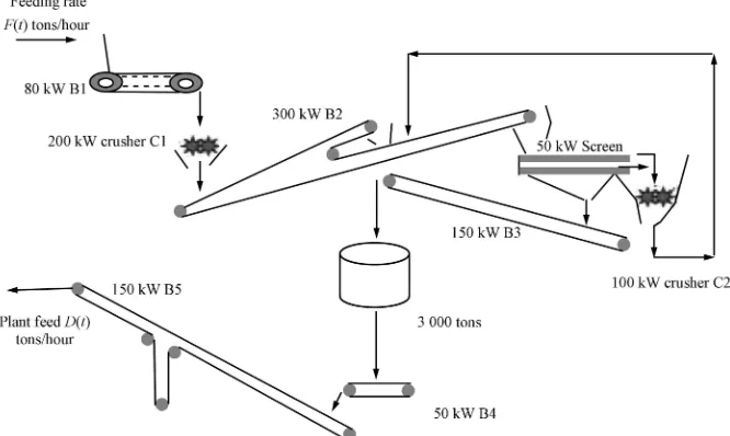
Fig. 1. Mineral processing system.
A. Mineral Processing System
In the mineral processing system in Fig. 1, minerals are fed at the rate of F(t)tons/hour to the 80 kW conveyor belt B1. From the 200 kW crusher C1, these minerals are further transported by conveyor belt B2 to a 50 kW screen system. After the screen, smaller size minerals go to the 150 kW conveyor belt B3, larger size ones go to the 100 kW crusher C2 to be recrushed and then sent back to conveyor belt B2. Minerals from B3 are sent to a 3 000 ton stock silo, where they will be further supplied to the 50 kW conveyor belt B4 and from B4 to the 150 kW conveyor belt B5. The plant feed demand at the end of conveyor belt B5 isD(t)tons/hour. The question for this problem is to minimise electricity cost in terms of a time-of-use electricity tariff over the time interval
[t0, tN]. Discretise [t0, tN] as t0 < t1 <· · ·< tN, t1−t0= t2−t1=· · ·=tN−tN−1= ∆T.
The overall mineral processing energy system consists of conveyors B1, B2, B3, B4, B5; crushers C1, C2; and a screen. Define the on/off switching status functions for these system components as follows.uBi,k represents the on/off status of the i-th conveyor Biat thek-th time interval, withi= 1,2,3,4,5;
uC
1,k anduC2,k are the on/off status of crushers C1 and C2 at
thek-th time interval, respectively; anduS
k is the on/off status
of the screen at time k. The values of these switching status functions can only be 0 or 1, representing “off” or “on” status. Following the steps in Section II-A, the objective function to minimise electricity cost over [t0, tN] for a given electricity
tariff$pk/kWh,k= 1,· · ·, N, is written as:
min
N
X
k=1
pk(80uB1,k+ 200uC1,k+ 300uB2,k+ 150uB3,k+
100uC2,k+ 50uSk + 50uB4,k+ 150uB5,k)∆t. (11)
Note in the mineral process, conveyors B1, B2, B3, crushers C1, C2, and the screen have the same operation schedule, i.e., they are switched on at the same time, and switched off at the same time. Similarly, conveyors B4 and B5 must also have
the same operating schedule in order to minimise energy cost. Therefore, the following equalities hold:
uB
1,k =uC1,k=uB2,k=uB3,k,=uC2,k=uSk,
uB
4,k =uB5,k, k= 1,· · ·, N.
(12)
From the mass balance relations, it is reasonable to assume that all minerals fed at conveyor B1 will be fed at the same rate F(t)tons/hour to the 3 000 ton stock silo; and similarly, the conveyor B4 must be fed at the rate of D(t) tons/hour from the stock silo. Then the following mass balance relation at the stock silo can be obtained:
Mk =Mk−1+F(k)−D(k), k= 1,· · ·, N, (13) whereM(k)represents the mass of minerals at the stock silo at time k, the initial mass M(0) is assumed to be given. Usually the stock silo has a certain capacity constraint for safety reasons, such as the stored minerals at any time must be within the range of 10 tons to 2 980 tons. Then the following constraints can be obtained.
10≤Mk≤2980, k= 1,· · ·, N. (14)
Now the optimisation problem (11)∼(14) can be solved to find an optimal on/off status control over the time interval
[t0, tN]. An MPC algorithm can be easily designed to optimise
the on/off scheduling status over the time interval [tk, tN+k].
We would however leave the MPC applications in the follow-ing two subsections.
B. Water Purification System
by pumps K1, K2 and K3, each rated at 300 kW with the same capacity to pump 22 mL/day. Water from R1 to R3 is pumped by pumps G1, G2 and G3, each rated at 275 kW with the capacity to pump 10 mL/day. R2 and R3 are also supplied by a water utility called Randwater at the cost of ZAR 2.98/kL, where ZAR represents the South African currency rand. R3 is also supplied by boreholes at a rate of 10 mL/day with the cost of ZAR 0.30/kL; water cost from R1 to R2 and R3 has the same rate ZAR 1.03/kL. Pumps K3 and G3 are used as back-up pumps and usually are switched off. To simplify the model, it is assumed in [10] that pump G2 keeps running continuously, and pump K2 is chosen as the control object, and the following optimisation model is obtained.
minut,z
T
P
t=1
utpct+PSzC
s.t. Lt
1=L01+
tP−1
k=1
(FLOWINk1−ukFLOWOUTk1)
1.3mL≥Lt
1≥0.2 mL, t= 1,· · ·, T,
kSP+S t=1+kS
utP−P zs≤0, k= 0,· · ·,(TS −1),
(15) where the two parts in the objective function represent the energy charge and the maximum demand charge, respectively, Lt
1 is the volume of water in reservoir R1 which should always be between 0.2 mL and 1.3 mL for capacity limit and safety reasons, ut is the on/off status of pump K2, S = 2,
C = ZAR 66.5/kW, P=300 kW, andzis an intermediate variable which helps to calculate the maximum demand. It is obvious that the constraint about water levels can be derived from the general mass balance constraint in (6). Therefore, this model is a direct application of the general principles in the previous section. Reference [11] further applies MPC to the above problem over a moving horizon of 24 hours. Percentage of savings under benchmarks with the assumptions for real value ut ∈ [0,1], the open loop control with binary values of ut,
and MPC with binary values of ut are compared, and Fig. 3
illustrates that MPC and open loop controller have almost the same amount of savings. However, if there is a positive random inflow disturbance, i.e., FLOWINt1is replaced by FLOWINt1+ 0.2∼FLOWINt1×r(m)withr(m)a random number between 0 and 1, then the open loop solution will violate the reservoir allowable capacity 1.3 mL at R1 as shown in Fig. 4. Therefore, MPC method will be very helpful to provide a robust solution. The model in (15) can be further improved by incorporating more control variables and constraints. For instance, all the four pumps G1, G2, K1, K2 can be controlled simultaneously, and the customer water demand can also be considered so as to minimise the supplementary water supply which has a high cost of R2.98/kL.Then the objective function in (15) can be revised as follows.
T
P
t=1
(P4
i=1 ut
ipct+ 2.98Rt2+ 2.98Rt3) +PSzC, (16)
whereutirepresents the on/off status of the four pumps at time t,Rt2andRt3are the amount of supplementary water supplied from the water company Randwater at timetto the reservoirs R2 and R3, respectively. Assume that customer demand at time
tfrom reservoirs R2 and R3 areDt
2 andDt3, respectively. The water levels in R2 and R3 will satisfy similar constraints like those for R1 in (15). For example, the water in R2 must satisfy the following constraint.
maximum water capacity of R2≥Lt2≥ minimum water capacity of R2, Lt
2=Lt2−1+ (ut1+ut2)v1+Rt2−Dt2,
[image:5.612.352.521.168.411.2](17)
[image:5.612.55.301.219.312.2]Fig. 2. A water pumping system[11].
Fig. 3. Comparison of the savings by open loop controller and MPC[11].
Fig. 4. Reservoir level constraint violation of open loop
controllers[11].
[image:5.612.359.512.570.686.2]pumped by pump K1 per unit time, which remains the same for pump K2;Dt
2is the customer water demand from reservoir R2. Note that electricity suppliers often have incentives to industrial customers who are willing to reduce evening peak load, therefore it is proposed to expect the four pumps K1, K2, G1, G2 are not switched on simultaneously at the evening peak period 18:00-20:00. This can be easily formulated as the following logic correlations:
ut
1+ut2+ut3+u4t ≤3, for t∈(18:00, 20:00). (18) The new model can be further applied in the MPC approach to achieve better energy savings.
C. Plant Maintenance Optimal Scheduling
Generator maintenance optimal scheduling has been studied by many authors; see references listed in [414]. Similar main-tenance scheduling problems exist in many industrial plants. Starting from the model in [14], this subsection proposes an optimisation model to characterise the general plant mainte-nance scheduling problem.
Assume a plant consists ofndivisions (or units) which need to be regularly maintained. Consider a fixed time period ofm days over which an optimal maintenance schedule needs to be found. For simplicity, assume that each division needs to undergo one and only one maintenance within them days.
Lett represent time (in days), andxi,t be the maintenance
state of the i-th division on the t-th day, with xi,t = 1
representing thei-th division is under maintenance on thet-th day, while xi,t = 0 has the converse meaning. Defineyi,t to
be the start up state, withyi,t equal to 1 implying that thei-th
division has been finished maintenance at time (t−1)and is started to work normally at timet.
The objective is to minimise maintenance cost by noting the fact that each division will deliver profits at any given time, and its closing down for maintenance will cause not only the maintenance cost but also the loss of the corresponding profits. For this purpose, assume that $pi,t is the profit produced by
the i-th division on the t-th day if it is operating normally. Assume that the maintenance cost for division i is $ai per
day, the starting up cost of divisioniis$bi. Then the objective
function is formulated below.
minJ =
n
X
i=1
m
X
t=1
(aixi,t+biyi,t−pi,txi,t). (19)
Note that a division under maintenance cannot be started. Therefore the following constraint is obvious.
xi,t+yi,t≤1, 1≤t≤m. (20)
Equation (21) means that the maintenance for division i needs ki days within the m days, while (22) implies that
whenever the maintenance of division istarts, it will take ki
consecutive days and no interruption is allowed.
m
X
t=1
xi,t=ki, 1≤i≤I. (21)
T−Pki+1
t=1 xi,txi,t+1. . . xi,t+ki−1= 1, 1≤i≤I.
(22)
The maintenance on these divisions may be subject to certain logic correlations. For instance, the first two divisions cannot be maintained together (i.e., at least one of them must be working). This can be written as the following constraint:
x1,t+x2,t≤1, 1≤t≤m. (23)
Other types of logic correlation constraints can be formulated following the formulae in Section II-A.
The number of maintenance crew needed at any mainte-nance instant must not exceed the number of available crews:
n
P
j=1
(1−xj,t−1)xj,t. . . xj,t+q−1Mjq≤At+q−1,
1≤q≤ki, 2≤t≤m−ki+ 1,1≤i≤n,
(24)
where Miq is the number of crew needed for the q-th day of maintenance for the i-th division, and At is the available
number of crew at timet.
There might also be a least requirement on the daily profit produced even some of the divisions are under maintenance. For example, the following inequality indicates that the mini-mum daily profit should be at least$A.
n
P
i=1
pi,t(1−xi,t)≥A, 1≤t≤m. (25)
Other system requirements can be added to the above model in order to determine a practically implementable scheduling plan.
The above optimisation model is formulated over the time period from t= 1 tot =m, and it is easily changed into a time period starting from any day for the MPC applications. Dynamic market impact on the profit pi,t can be easily
captured in the MPC approach, therefore, the MPC application will greatly improve the reliability of the above maintenance scheduling model.
IV. CONCLUSIONS
This paper summarises general techniques in energy system operation efficiency modelling and the corresponding model predictive control approach to the obtained energy optimi-sation models. Examples from mineral processing and plant maintenance are used to illustrate the modelling process, case study on a water pumping system shows further the effectiveness of the model predictive control approach.
REFERENCES
[1] Xia X H, Zhang J F. Energy efficiency and control systems-from a POET perspective. In: Proceeding of the 2010 Conference on Control Methodologies and Technology for Energy Efficiency. Portugal: IFAC, 2010. 255−260
[2] Xia X H, Zhang J F, Cass W. Energy management of commercial buildings — A case study from a POET perspective of energy efficiency.
Journal of Energy in Southern Africa, 2012, 23(1): 23−31
[4] Xia X H, Zhang J F. Energy auditing-from a POET perspective. In: Proceedings of the 2010 International Conference on Applied Energy. Singapore, 2010. 1200−1209
[5] Allg¨ower F, Zheng A. Nonlinear Model Predictive Control. Berlin: Birkh¨auser Verlag, 2000.
[6] Garc´ıa C E, Prett D M, Morari M. Model predictive control: theory and practice – A survey.Automatica, 1989, 25(3): 335−348
[7] Qin S J, Badgwell T A. A survey of industrial model predictive control technology.Control Engineering Practice, 2003, 11(7): 733−764
[8] Ashok S. Peak-load management in steel plants.Applied Energy, 2006,
83(5): 413−424
[9] Wu T Y, Shieh S S, Jang S S, Liu C C L. Optimal energy management integration for a petrochemical plant under considerations of uncertain power supplies. IEEE Transactions on Power Systems, 2005, 20(3): 1431−1439
[10] Badenhorst W, Zhang J F, Xia X H. Optimal hoist scheduling of a deep level mine twin rock winder system for demand side management.
Electric Power Systems Research, 2011, 81(5): 1088−1095
[11] van Staden A J, Zhang J F, Xia X H. A model predictive control strategy for load shifting in a water pumping scheme with maximum demand charges.Applied Energy, 2011, 88(12): 4785−4794
[12] Zhang H, Xia X H, Zhang J H. Optimal sizing and operation of pumping systems to achieve energy efficiency and load shifting.Electric Power Systems Research, 2012, 86: 41−50
[13] Xia X H, Zhang J F, Elaiw A. An application of model predictive control to the dynamic economic dispatch of power generation.Control Engineering Practice, 2011, 19(6): 638−648
[14] Ekpenyong U E, Zhang JF, Xia X H. An improved robust model for generator maintenance scheduling. Electric Power Systems Research, 2012, 92: 29−36
[15] Yamayee Z A. Maintenance scheduling: description, literature survey, and interface with overall operations scheduling.IEEE Transactions on Power Apparatus and Systems, 1982, 101(8): 2770−2779
[16] Zhang J F, Xia X H. A model predictive control approach to the peri-odic implementation of the solutions of the optimal dynamic resource allocation problem.Automatica, 2011, 47(2): 358−362
Xiaohua Xia Professor in the Department of
Elec-trical, Electronic, and Computer Engineering at the University of Pretoria, South Africa, and the director of both the Centre of New Energy Systems and the National Hub for Energy Efficiency and Demand-side Management. He was academically affiliated with the University of Stuttgart, Germany, the Ecole Centrale de Nantes, France, and the National Uni-versity of Singapore before joining the UniUni-versity of Pretoria in 1998. He is a fellow of IEEE, a member of the Academy of Science of South Africa, and a fellow of the South African Academy of Engineering. He has been an associate editor or an editorial board member forAutomatica, IEEE Transactions on Circuits and Systems II, IEEE Transactions on Automatic Control, Applied Energy,and specialist editor (control) of theSAIEE Africa Research Journal.
Jiangfeng Zhang obtained the B. Sc. and Ph. D. in
![Fig. 3.Comparison of the savings by open loop controller andMPC[ 1 1 ] .](https://thumb-us.123doks.com/thumbv2/123dok_us/1619272.114985/5.612.359.512.570.686/fig-comparison-savings-open-loop-controller-andmpc.webp)
