Effective Feature Extraction and
Data Reduction in Remote Sensing
Using Hyperspectral Imaging
Jinchang Ren, Jaime Zabalza, Stephen Marshall, Jiangbin Zheng
With numerous and contiguous spectral bands acquired from visible light (400nm-1000nm) to (near) infrared (1000nm-1700nm and over), hyperspectral imaging (HSI) can potentially identify different objects by detecting minor changes in temperature, moisture and chemical content. As a result, HSI has been widely applied in a number of application areas, including remote sensing [1]. HSI data contains 2-D spatial and 1-D spectral information, and naturally forms a 3-D hypercube with a high spectral resolution in nanometers that enables robust discrimination of ground features. However, new challenges arise in dealing with extremely large datasets. For a hypercube with relatively small spatial dimension of 600×400 pixels at 16 bits-per-band-per-pixel, the data volume becomes 120M bytes for 250 spectral bands. In some cases, this large data volume can be linearly increased when multiple hypercubes are acquired across time to monitor system dynamics in consecutive time instants. When the ratio between the feature dimension (spectral bands) and the number of data samples (in vector based pixels) is vastly different, high dimensional data suffers from the well-known curse of dimensionality. For feature extraction and dimensionality reduction, Principal Components Analysis (PCA) is widely used in HSI [2], where the number of extracted components is significantly reduced compared to the original feature dimension, i.e. the number of spectral bands. For effective analysis of large scale data in HSI, conventional PCA faces three main challenges: (i) To obtain the covariance matrix in extremely large spatial dimension, which can lead to software tools such as Matlab running out of memory; (ii) To cope with the high computational cost required for analysis of large datasets; and (iii) To retain locally structured elements which only appear in a small number of bands (namely local structures) for improved discriminating ability when feature bands are globally extracted as principal components. This article discusses several variations and extensions of conventional PCA to address the aforementioned challenges. These variations and extensions include slicing the HSI data for efficient computation of the covariance matrix similarly done in 2D-PCA analysis [3], and grouping the spectral data to preserve the local structures and further speed-up the process to determine the covariance matrix [4]. In addition, we also discuss some non-PCA based approaches for feature extraction and data reduction, based on techniques such as band selection, random projection, singular value decomposition and machine learning approaches such as support vector machine (SVM) [2, 5, 6].
FEATURE EXTRACTION USING PCA AND ITS VARIATIONS
PCA has been widely used for unsupervised feature extraction and data reduction [2, 7]. Through orthogonal projection and truncation of the transformed feature data, PCA can successfully remove correlation inherent in the data.
Eigen-decomposition is followed by data projection to determine the principal components. Due to the extremely large size of S, which can be over 100k bytes, practical difficulties arise when directly determining Λ from I. To solve these problems, 2D-PCA inspired data slicing PCA [3] along with segmented PCA (Seg-PCA) [4] are used.
[Fig1] Diagrams of conventional PCA in comparison with the data slicing PCA (SPCA) and Segmented PCA (Seg-PCA)
Data Slicing PCA (SPCA)
Rather than taking all spectral vectors in I together, SPCA (Fig. 1) treats each spectral vector In
separately when determining the corresponding covariance matrix Λ, where n[1,S]. For each 1
F
n
I , its associated partial covariance matrix is obtained as F F n
n
T
I
I , and the overall covariance matrix Λ is determined as the sum of all partial covariance matrices by
S RC
n n n
S 1 T 1
I I
Λ
(1)
SPCA is equivalent to PCA in determining the covariance matrix. The fundamental difference is that the calculation of Λ is implemented by a series of S independent partial covariance matrices. As such, the memory requirement is reduced from F×S to F×1. In addition to this, these partial covariance matrices can be separately calculated in parallel to improve efficiency.
Segmented PCA (Seg-PCA)
Although the spectral data in HSI naturally form long vectors, the input spectral data can be grouped to produce a series of small vectors for fast calculation of PCA in each group whilst enabling extraction of local structures from each group. As shown in Fig 1, in Seg-PCA each of the S spectral vectors is grouped to form k sub-vectors. For each sub-vector, the size of its covariance matrix is reduced to nknk.
For a particular group b[1,k], let T 2
1 ... ]
[ m m nm b
mb i i ib
Then, Λb can be determined as follows.
S
m mb mb b S 1
T 1
i i
Λ (2)
where again S denotes the spatial size of the hypercube. Also note that imbiTmb is the partial covariance
matrix obtained from the grouped spectral vector imb. For a given spectral vector F1
n
i , conventional PCA extracts all the principal components from the F bands. In contrast, Seg-PCA divides in into H groups and ensures that variable numbers of components are extracted from each group. As a result, Seg-PCA has the potential to preserve some local spectral structures, which are non-dominant and thus are discarded in conventional PCA. Such local structures provide additional values to Seg-PCA for superior discrimination ability as explained below.
In Seg-PCA, as illustrated in Fig. 1, each spectral vector of F bands is grouped into H groups. When H 1, Seg-PCA defaults to SPCA, which is equivalent to the conventional PCA. In fact, the performance of the Seg-PCA is strongly dependent on how the bands are grouped, as it affects how much additional information can be extracted to improve the conventional PCA.
In one particular case where all groups contain the same number of W bands, HWF, the covariance matrices from different groups share the same dimension. As a result, they can be summed to form one covariance matrix ΛSegPCA. This can further simplify the eigen-decomposition procedure for better efficiency, as only one matrix rather than k must be processed.
k b b PCA
Seg 1Λ
Λ (3)
In conventional PCA, using SPCA for example, the covariance matrix in (1) can be rewritten as follows, where in [a1n,a2n,...,aHn].
S n T Hn Hn T n Hn T n Hn T Hn n T n n T n n T Hn n T n n T n n n S n n SPCA S S 1 2 1 2 2 2 1 2 1 2 1 1 1 T 1 1 1 a a a a a a a a a a a a a a a a a a i i Λ (4)For the particular case in Seg-PCA where all groups have the same number of bands, the covariance matrix can be further derived as:
S n T Hn Hn T n n T n n Sn n n PCA
Seg
S
S 1 1 1 1 2 2
1 1 a a a a a a I I
Λ T (5)
From (4) and (5), it is straightforward to demonstrate that ΛSegPCA is formed by accumulating the
W
FEATURE EXTRACTION USING NON-PCA BASED APPROACHES
For non-PCA based feature extraction and dimensionality reduction, the most commonly used approaches are based on band selection [5], machine learning [6] and steepest ascent search [7]. As adjacent spectral bands in hyperspectral imaging usually contain a large degree of redundant information, these approaches tend to select individual spectral bands rather than PCA components for data classification.
In these approaches, bands that contain less discriminatory information are discarded, which results in a much reduced number of remaining bands. Usually, the discriminatory information is reflected by how different a band is in comparison to adjacent bands. To determine the degree of similarity between two (band) images, a number of approaches can be used including distance measurement, mutual information and the structural similarity measurement (SSIM) [2, 5].
For any two band images Am and An, the simplest distance-based similarity is given below to measure an average distance/similarity over all pixels:
X i Yi m n X i Y i n m n m d j i A j i A j i A j i A A A S 1 1 1 1 ))] , ( ), , ( [max( | ) , ( ) , ( | 1 ) , ( (6)
where 0 and (i,j) are the spatial coordinate indices of the two images satisfying i[1,X] and
] , 1
[ Y
j ; XY denotes the spatial dimension of the band images.
In contrast, mutual information based similarity is determined by the image histograms [2, 5]. By treating the spectral images as random variables, their associated mutual information can be determined as follows:
) , ( ) ( ) ( ) ,
(Am An H Am H An H Am An
I (7)
where H(Am) and H(An) are the entropy of Am and An, and H(Am,An) is their joint entropy.
m A am p a p a
A
H( ) ( )log ( ) (8)
The structural similarity measurement (SSIM) [8] contains three factors, including consistency in terms of luminance l(Am,An), contrast c(Am,An)and structure s(Am,An) defined as follows.
1 2 2 1 2 ) , ( C C A A l n m n m n
m
2 2 2 2 2 ) , ( C C A A c n m n m n
m
3 3 ) , ( C C A A s n m mn n m (9) ) , ( ) , ( ) , ( ) ,
(Am An l Am An c Am An s Am An
SSIM (10)
where (m,n) and (m, n) are the mean intensity and the standard deviation of the band images
m
A and An , respectively; C1 -C3 are constants; and ,, are non-negative weights. In the particular case where 1 and C2 2C3, SSIM can be further simplified as
) )( ( ) 2 )( 2 ( ) , ( 2 2 2 1 2 2 2 1 C C C C A A SSIM n m n m mn n m n
m
Due to the inclusion of a consistency measurement in terms of luminance, contrast and structural similarity, SSIM is found to produce more consistent similarity measurements than distance and mutual information based approaches [9]. For the 92AV3C dataset as described in detail in the next section, SSIM-based band similarity maps are shown in Fig. 2. As can be seen, bands are naturally divided into similar groups, with exceptions to bands just over 100 and 150 where adjacent bands show low similarity to each other. These are noisy bands which contain little useful information, hence the low correlation with adjacent bands.
50 100 150 200
20
40
60
80
100
120
140
160
180
200
220
0 0.1 0.2 0.3 0.4 0.5 0.6 0.7 0.8 0.9 1
[Fig2] The correlation matrix among the band images of the 92AV3C dataset.
Based on the similarity maps above, band groups and the key bands can be easily determined by thresholding [3] or Jeffries-Matusita interclass distance [7] with the steepest ascent search strategy [2, 7]. For machine learning based approaches, ground-truth information is usually used to determine the discriminatory ability of bands in any classification based tests.
PERFORMANCE EVALUATION AND ANALYSIS
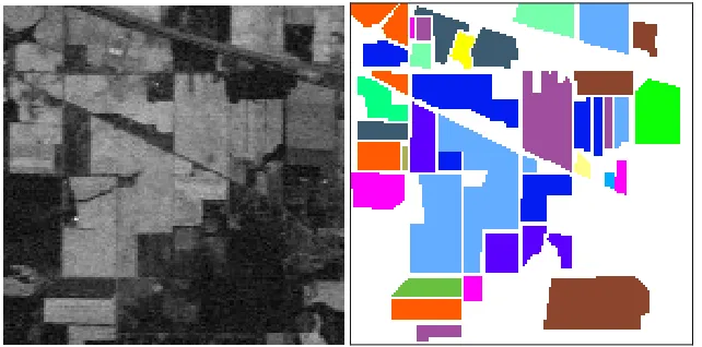
We compare the performance of SPCA and Seg-PCA with conventional PCA using the publicly available hyperspectral dataset 92AV3C from the original Indian Pines [10]. The 92AV3C dataset was collected by the AVIRIS instrument over an agricultural study site in Northwest Indiana [10] for land cover classification in remote sensing applications. The hyperspectral dataset contains 220 spectral reflectance bands in the wavelength range of 400nm to 2500nm, and the spatial size is 21025 (145×145) pixels. The dataset contains different land cover classes corresponding to agriculture, forest, vegetation, and buildings. One sample band and the ground truth of the 16 land cover classes are illustrated in Fig. 3. Disregarding the white regions which are unclassified background, the other coloured regions in the ground truth refer to alfalfa, corn (3 types), wheat, grass (3 types), oats, woods, soybeans (3 types), hay, and two others.
FEATURE EXTRACTION AND DATA CLASSIFICATION
SVM is the Radial Basis Function (RBF), whose parameters, the penalty (c) and the gamma (γ), were optimized in the training process through a grid search of possible combinations of these parameters.
As suggested in the literature [5, 7], the noisy bands covering the region of water absorption (104-108, 150-163, 220) are removed from the spectral vectors before applying PCA for feature extraction. To this end, the effective number of spectral bands for the datasets is reduced from 220 to 200. In total, four groups of features are used for comparison. The first is referred to as the Whole Spectral Band (WSB), in which the total 200 spectral bands are used directly as features. This is taken as a baseline approach for benchmarking. The remaining three groups use principal components as features, extracted from the conventional PCA, the SPCA and Seg-PCA approaches respectively.
For each group of features as samples, 10 experiments were carried out with data samples randomly selected for training and testing. No data sample overlap was allowed in the training set and testing set. The average testing result over these tests and the corresponding standard deviation of classification accuracy were obtained and reported below for evaluation and assessment.
[Fig 3] One sample band image (left) and the ground truth of land cover (right) of the 92AV3C dataset.
PERFORMANCE ASSESSMENT
We assess performance in terms of reduction of computation cost, memory requirement and improvement of classification accuracy.
The computation costs of the SPCA and Seg-PCA are compared against those of the conventional PCA in Table I, for the three stages involved, where S and K refer respectively to the number of samples (pixels) and the number of principal components extracted. Since the computational cost for PCA and SPCA is the same, they are put together to be compared with Seg-PCA. The saving factor of computational cost for Seg-PCA is H or H3 in comparison to conventional PCA and SPCA. With
10
H and K30, the number of Multiply-ACcumulates (MACs) required in PCA/SPCA is 9.75e8, where in Seg-PCA it is reduced to 9.67e7. In effect, the computational cost has reduced to 9.92%. In other words, Seg-PCA has achieved a saving factor of 10, i.e. an order of magnitude for the hyperspectral remote sensing dataset used.
TABLEI.COMPARISONS OF COMPUTATIONAL COST
Stages \ Approaches Covariance matrix Eigen problem Data projection PCA/SPCA O(S H2 W2) O(H3 W3) O(S HWK)
Seg-PCA O(S H W2) O(HW3) O(S WK)
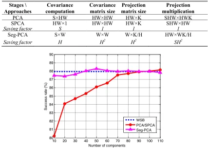
[image:6.612.160.481.262.421.2]In Table II, memory requirements for PCA, SPCA and Seg-PCA over different stages are compared. SPCA only reduces memory requirement in the first stage when the covariance matrix is obtained. The other two stages require the same amount of memory as the conventional PCA. Seg-PCA has significantly lower memory requirements, and the minimum saving factor achieved is
2
H . When H 10, Seg-PCA only requires 1% of the memory compared to the conventional PCA.
TABLEII.COMPARISON OF MEMORY REQUIREMENTS IN PCA,SPCA AND SEG-PCA AT DIFFERENT STAGES
Stages \ Approaches
Covariance computation
Covariance matrix size
Projection matrix size
Projection multiplication
PCA S×HW HW×HW HW×K SHW×HWK
SPCA HW×1 HW×HW HW×K SHW×HW
Saving factor S 1 1 1
Seg-PCA S×W W×W W×K/H HW×WK/H
Saving factor H H2 H2 SH2
10 20 30 40 50 60 70 80 90 100 110
80 81 82 83 84 85 86 87 88 89 90
Number of components
Su
cc
es
s
ra
te
(%
)
WSB PCA/SPCA Seg-PCA
[Fig 4] Classification results for the 92AV3C dataset from PCA/SPCA and Seg-PCA in benchmarking with WSB approach under various numbers of principal components used, where the training ratio is 30%.
With local structures extracted over the spectral domain, Seg-PCA has great potential to improve the efficacy in feature extraction resulting in higher discrimination power and better classification. With H 10(W 20), the classification results using various numbers of principal components are plotted in Fig. 4, where K covers a large range from 10 to 110. First, Seg-PCA is found to consistently outperform conventional PCA (and also SPCA). As can be seen, Seg-PCA significantly improves on the conventional PCA when the number of components is less than 110, i.e. 50% of the dimensionality of original features. When K is 10 and over, Seg-PCA achieves comparable or even slightly better results in comparison to WSB for classification, a significant advantage for feature extraction as the dimensionality of features used in WSB is 200.
Non-PCA based approaches
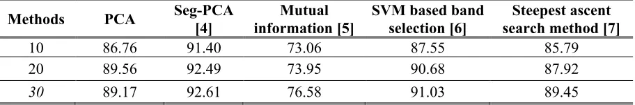
[image:7.612.91.518.187.491.2]based methods. Again SVM is used as the preferred classifier yet under 60% training ratio. The results are summarised in Table III for comparison. As one can see, PCA based approaches have generated reasonably good results, where Seg-PCA is found to be the best among the five approaches evaluated. SVM based approach outperforms conventional PCA and the steepest ascent search based approach, and mutual information based approach is found to be the poorest performing in this group of tests.
TABLEIII.COMPARISON OF THE OVERALL ACCURACY OF DIFFERENT APPROACHES UNDER VARIOUS NUMBER OF FEATURES USED FOR CLASSIFICATION
Methods PCA Seg-PCA [4]
Mutual information [5]
SVM based band selection [6]
Steepest ascent search method [7]
10 86.76 91.40 73.06 87.55 85.79
20 89.56 92.49 73.95 90.68 87.92
30 89.17 92.61 76.58 91.03 89.45
Effect of Noise
Due to atmospheric water absorption and other effects, the hyperspectral images obtained may contain severe noise, where the corresponding band image is effectively useless as it has no correlation to any adjacent bands (see in Fig. 2). As a result, noise removal becomes a very important issue. Without noisy band removal, the classification accuracy achieved for the 92AV3C dataset by PCA with 10 components is only around 70%, in comparison to nearly 87% obtained in Table III. Furthermore, some researchers also apply noise removal in the spatial domain, using the known wavelet shrinkage approach [12]. After removal of the noisy bands, it is found that this pre-processing can further improve the overall classification accuracy by 2-3% [12].
CONCLUSION
Although PCA has been widely used for feature extraction and data reduction, it suffers from three main drawbacks: high computational cost, large memory requirement and low efficacy in processing large datasets such as HSI. This column analysed two variations of PCA, namely SPCA and Seg-PCA. Seg-PCA can further improve classification accuracy whilst significantly reducing the computational cost and memory requirement, without requiring prior knowledge. There is potential to apply similar feature extraction and data reduction techniques in application areas beyond HSI when analysis of large dimensional datasets is required such as magnetic resonance imaging (MRI) and digital video processing.
RESOURCES
For hyperspectral remote sensing, a series of sensors have been applied in the world, which include AVIRIS [10], ROSIS [13] and HYDICE [10] as well as many others such as TRWIS, CASI, OKSI AVS, MERIS, Hyperio, HICO, CHRIS, NEON and TERN. Detailed specifications in terms of the spectral range and spectral/spatial resolution etc for these sensors are summarised in [14, 15].
[image:8.612.80.536.177.253.2]AUTHORS
Jinchang Ren ([email protected]) is the Deputy Director of Hyperspectral Imaging Centre in the University of Strathclyde, Glasgow, U.K.
Jaime Zabalza ([email protected]) is currently working towards his PhD. at the Department of Electronic and Electrical Engineering, University of Strathclyde.
Stephen Marshall ([email protected]) is a Professor with the Department of Electronic and Electrical Engineering in Strathclyde, and a Fellow of the IET.
Jiangbin Zheng ([email protected]) is currently a Professor in School of Software and Microelectronics, Northwestern Polytechnical University, Xi’an, China.
REFERENCES
[1] R. Dianat and S. Kasaei, “Dimension reduction of optical remote sensing images via minimum change rate deviation method,” IEEE Trans. Geosci. Remote Sens., 48(1): 198-206, Jan. 2010. [2] X. Jia, B.-C. Kuo, M. Crawford, “Feature mining for hyperspectral image classification, ” Proc. of
IEEE, vol. 101, no. 3, pp. 676-697, March 2013.
[3] J. Yang, D. Zhang, A. F. Frangi, and J-Y Yang, “Two-Dimensional PCA: A new approach to appearance-based face representation and recognition,” IEEE Trans. PAMI, vol. 26, no.1, pp. 131-137, January 2004
[4] X. Jia, and J.A. Richards, “Segmented principal components transformation for efficient hyperspectral remote sensing image display and classification,” IEEE Trans. Geosci. Remote Sens, vol. 37, pp. 538-542, 1999.
[5] B. Guo, S. Gunn, R. Damper, and J. Nelson, “Band selection for hyperspectral image classification using mutual information,” IEEE Geoscience and Remote Sensing Letters, Vol. 3, no. 4, pp. 522-526, 2006
[6] M. Pal, and G. M. Foody, “Feature selection for classification of hyperspectral data by SVM,” IEEE Trans. Geoscience and Remote Sensing, Vol. 48, no. 5, pp. 2297-2307, 2010
[7] F. Melgani and L. Bruzzone, “Classification of hyperspectral remote sensing images with SVMs,” IEEE Trans. Geosci. Remote Sens, vol. 42, no. 8, pp. 1778–1790, August 2004.
[8] Z. Wang, A. C. Bovik, H. R. Sheikh, and E. P. Somoncelli, “Image quality assessment: from error visibility to structural similarity,” IEEE Trans. Image Proc., vol. 13, no. 4, pp. 600-612, 2004 [9] D. P. Widemann, Dimensionality Reduction for Hyperspectral Data, PhD thesis, University of
Maryland, 2008.
[10]Pursue's univeristy multispec site: June 12, 1992 aviris image north-south flightline, indiana [Online], available : https://engineering.purdue.edu/~biehl/MultiSpec/hyperspectral.html
[11]bSVM multiclass classifier 2.08, released on June 18, 2012 [Online], available:
http://www.csie.ntu.edu.tw/~cjlin/bsvm/
[12]B. Demir, S. Erturk, and M. K. Gullu, “Hyperspectral image classification using denoising of intrinsic mode functions,” IEEE Geosc. & Remote Sens. Letters, vol. 8, no. 2, pp. 220-224, 2011 [13]Online datasets: http://www.ehu.es/ccwintco/index.php/Hyperspectral_Remote_Sensing_Scenes
[14]http://www.gisresources.com/fundamemtals-of-hyperspectral-remote-sensing_2/