City, University of London Institutional Repository
Citation
:
Howe, J. M. (1997). Two loop detection mechanisms: a comparison. Paper presented at the International Conference on Analytic Tableaux and Related Methods (TABLEAUX'97), 13 - 16 May 1997, Pont-a-Mousson, France.This is the unspecified version of the paper.
This version of the publication may differ from the final published
version.
Permanent repository link:
http://openaccess.city.ac.uk/1707/Link to published version
:
Copyright and reuse:
City Research Online aims to make research
outputs of City, University of London available to a wider audience.
Copyright and Moral Rights remain with the author(s) and/or copyright
holders. URLs from City Research Online may be freely distributed and
linked to.
City Research Online: http://openaccess.city.ac.uk/ [email protected]
Two Loop Detection Mechanisms: a Comparison
Jacob M. Howe
Computer Science Division
University of St Andrews, Scotland, KY16 9SS
Abstract. In order to compare two loop detection mechanisms we describe two
calculi for theorem proving in intuitionistic propositional logic. We call them both
MJ Hist
, and distinguish between them by description as ‘Swiss’ or ‘Scottish’. These calculi combine in different ways the ideas on focused proof search of Her-belin and Dyckhoff & Pinto with the work of Heuerding et al on loop detection. The Scottish calculus detects loops earlier than the Swiss calculus but at the ex-pense of modest extra storage in the history. A comparison of the two approaches is then given, both on a theoretic and on an implementational level.
1
Introduction
The main interest of this paper is the comparison of the two loop detection mechan-isms described below. In order to do this we illustrate their use on the permutation-free sequent calculus
MJ
for the propositional fragment of intuitionistic logic. This gives calculi whose implementations are suitable for theorem proving.Backwards proof search and theorem proving with a standard cut-free sequent cal-culus, Gentzen’s
LJ
, for the propositional fragment of intuitionistic logic is inefficient because of three problems. Firstly, the proof search is not in general terminating, due to the possibility of looping. Secondly, it will produce proofs which are essentially the same; they are permutations of each other, and correspond to the same natural deduc-tion. Thirdly, there are choice points where it has to be decided which of several rules to apply and where to apply them.The sequent calculus
MJ
for intuitionistic logic was introduced (with another name,LJT
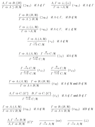
) by Herbelin in [7]. The propositional fragment of the calculusMJ
is displayed in Figure 1. This uses Girard’s idea of a special place for formulae in the antecedent, the stoup first seen in [6]. The calculus was developed by Dyckhoff and Pinto [3] be-cause it has the property that proofs are in 1–1 correspondence with the normal natural deductions ofNJ
.MJ
is a permutation-free sequent calculus; it avoids the problems of permutations in the cut-free sequent calculus of Gentzen. This removes the second of the problems. In this paper we are more interested in theorem proving than in proof search, hence the second problem is not directly relevant. But notice that permutations are avoided inMJ
by a focusing method — several choice points are removed. That is,MJ
partly addresses the third problem and hence is advantageous as a calculus for theorem proving. However, the na¨ıve implementation ofMJ
will lead to the possibility of looping.to be stored. Recent work by Heuerding et al [9] (the intuitionistic case of which is closely related to that of Gabbay in [5]) shows how to use a ‘history’ to prevent looping in a far more efficient way.
In this paper the history mechanism is developed in two ways and applied to
MJ
. Both the resulting calculi have advantages and disadvantages. These are discussed the-oretically and also pragmatically (in terms of the speed with which Prolog implement-ations give proofs). We call the new calculusMJ
Hist, the two varieties ‘Swiss’ and ‘Scottish’.
A;
)B
)A
B
( R
)
)
A
B!
C
AB!
C
( L
)
A !
C
A^B!
C
(^L1 )
B !
C
A^B!
C
(^L2 )
)
A
)B
)A
^B
(^ R
)
A;
)C B;
)C
A_B!
C
(_ L
)
)
A
)A
_B
(_ R
1 )
)
B
)A
_B
(_ R2
)
A;
A !B
A;
)B
(C
)A !
A
(
ax
)? !
A
(?)
Define:
A
A
?.A
,B
,C
are formulae. is a multiset of formulae.B
, is shorthand forfB
g[ , where[is multiset union.Sequent )
C
has context , goalC
and no stoup.Sequent A
[image:3.612.190.442.181.388.2]!
C
has context , goalC
and a single formula,A
, in the stoup.Fig. 1. Propositional Fragment of the calculus
MJ
.2
Calculi With Histories
In this section we first discuss the idea of the history mechanism, and then describe the two calculi. We shall conclude with a comparison of the two calculi.
2.1 The Use of Histories to Prevent Looping
.. ..
(
p
^p
)p
)p
.. ..
(
p
^p
)p
)p
(p
^p
)p
)p
^p
(^ R
)
(
p
^p
)p
p !p
(
ax
) (p
^p
)p
(p^p)p !
p
( L
)
(
p
^p
)p
)p
(C
)The sequent (
p
^p
)p
)p
may continue to occur in the proof tree for thissequent using the
MJ
calculus. We can see that there is a loop: we need a mechanical way to detect such loops.One way to do this is to add a history to each sequent. The history is the set of all sequents that have occurred so far on the branch of a proof tree. After each backwards inference the new sequent (without its history) is checked to see whether it is a member of this set. If it is we have looping and backtrack. If not the new history is the extension of the old history by the old sequent (without its history), and we try to prove the new sequent, and so on. Unfortunately this method is inefficient as it requires long lists of sequents to be stored by the computer, and all of this list has to be checked at each stage. When the sequents are stored we are keeping far more information than is necessary. Efficiency would be improved by cutting down the amount of storage and checks to the bare minimum needed to prevent looping.
The basis of the reduced history is the realisation (as in [9]) that one need only store goal formulae in order to loop-check. The rules of
MJ
are such that the context cannot decrease; once a formula is in the context it will be in the context of all sequents above it in the proof tree. For two sequents to be the same they obviously need to have the same context. Therefore we may empty the history every time the context is extended. All we need store in the history are goal formulae. If we have a sequent whose goal is already in the history, then we have the same goal and the same context as another sequent, that is, a loop.There are two slightly different ways of doing this. There is the straightforward extension and modification of the calculus described in [9] (which we call a ‘Swiss history’). The other approach involves storing slightly more formulae in the history, but detects loops more quickly. This we describe as the ‘Scottish history’; it can, in many cases, be much more efficient than the Swiss method.
2.2 The Swiss History
Before continuing, we should point out that the calculus we describe here as Swiss is significantly different from the one in [9]. This is partly due to our use of
MJ
as a base calculus, and partly because we are trying to focus on the history mechanism, hence we have not included the subsumption checks that the calculus in [9] uses.The Swiss-style calculus
MJ
Histis displayed in Figure 2. Let us make some gen-eral points about it (which will apply to the Scottish
MJ
Histas well). We have given explicit rules for negation (which are just special cases of the rules for implication) for the sake of completeness of connectives. Also, notice that there are two rules for(
These correspond to the two cases where the new formula is or is not in the context. As noted above (inx2.1) this is very important for
MJ
Hist
. Also note that the number of formulae in the history is at most equal to the length of the formula we check for provability.
The loop checking due to the history in the calculus works in a similar way to that ofIPC
RP ^;!
SU
in [9]. A sequent is matched against first the conclusions of right rules until the goal formula is either a propositional variable, falsum, or a disjunction (note that disjunction isn’t covered in [9], and requires special treatment). This is ensured by condition?
on rule(
C
). Then a formula from the context is selected and placed in thestoup by the(
C
)rule, the sequent is then matched against stoup formulae of left rules(this focusing does not occur in [9]). The history mechanism is used to prevent looping in the(
L
)rule (and similarly in the(: L
)rule). The left premiss of the rule has the
same context as the conclusion, but the goal is generally different. If the goal,
C
, of the conclusion is not in the history,H, we storeC
inHand continue backwards proofsearch on the left premiss. Alternatively,
C
might already be inH. In this case there is aloop, and so this branch is not pursued. We backtrack and look for a proof in a different way.
There is another place where the rules are restricted in order to prevent looping. This is the condition placed on the(_
L
)rule. For the( R
)rule (which attempts to extend
the context) there are two cases corresponding to when the context is and when it is not extended. Something similar is happening in the(_
L
)rule. In both the premisses of the
rule a formula may be added to the context. If both contexts really are extended, then we continue building the proof tree. If one or both contexts are not extended then the sequent with the non-extended context,
S
, will be the same as some sequent at a lesser height in the proof tree — there is a loop. This is easy to see: since the context and goal ofS
are the same as that of the conclusion, the sequent before the stoup formula (or a formula containing it as a subformula) was selected into the stoup must be the same asS
.We now state the equivalence theorem. This is done in two stages.
Theorem 1 The calculi
MJ
andMJ
Hist(without
?
) are equivalent. That is, a sequentS
is provable inMJ
if and only ifS
;(the sequent with the empty history) is provablein
MJ
Hist(without
?
).PROOF:(Sketch) The(direction is straightforward.
To prove the)direction we take an
MJ
proof tree and use it to build anMJ
Histproof tree.
We start at the root, )
A
inMJ
and we have root )A
;fA
ginMJ
Hist. Given a fragment of
MJ
proof tree with corresponding fragment ofMJ
Histproof tree, we look at the next inference in the
MJ
tree. We have a recipe which we can use to build a fragment ofMJ
Histproof tree corresponding to a strictly larger fragment of the
MJ
proof tree.A;
)B
; )A
B
;H( R1
) if
A =
2)
B
;H )A
B
;H( R2
) if
A
2A;
)?; ):A
;H(: R1
) if
A =
2)?;H ):
A
;H(: R2
) if
A
2)
A
;(C;
H) B!
C
;H AB!
C
;H( L
) if
C =
2H)
A
;(C;
H) :A!
C
;H (:L
) if
C =
2HA !
C
;H A^B!
C
;H (^L 1
)
B !
C
;H A^B!
C
;H (^L 2
)
)
A
;H )B
;H )A
^B
;H(^ R
)
A;
)C
;B;
)C
; A_B!
C
;H(_ L
) if
A =
2 andB =
2)
A
;H )A
_B
;H(_ R1
)
)
B
;H )A
_B
;H(_ R2
)
A;
A !B
;HA;
)B
;H (C
)?
A !
A
;H(
ax
)? !
A
;H(?)
? B
is either a propositional variable,?or a disjunction.A
,B
,C
are formulae, is a multiset of formulae, andHis a set of formulae.B;
is shorthand forfB
g[ .Sequent )
C
;Hhas context , goalC
, historyHand no stoup.Sequent A
!
C
;Hhas context , goalC
, historyHand stoupA
. [image:6.612.131.431.95.476.2]When the history has been extended we have parenthesised(
C;
H)for emphasis.Fig. 2. The propositional calculus
MJ
HistA;
)B
;fB
g )A
B
;H( R1
) if
A =
2A;
)?;f?g ):A
;H(: R1
) if
A =
2)
B
;(B;
H) )A
B
;H( R2
) if
A
2;
ifB =
2H)?;(?
;
H) ):A
;H(: R
2
) if
A
2;
if?2=
H)
A
;(A;
H) :A!
C
;H (:L
) if
A =
2H)
A
;(A;
H) B!
C
;H AB!
C
;H( L
) if
A =
2HA !
C
;H A^B!
C
;H (^L1 )
B !
C
;H A^B!
C
;H (^L2 )
)
A
;(A;
H) )B
;(B;
H) )A
^B
;H(^ R
) if
A =
2HandB =
2HA;
)C
;fC
gB;
)C
;fC
g A_B!
C
;H(_ L
) if
A =
2 andB =
2)
A
;(A;
H) )A
_B
;H(_ R1
) if
A =
2H)
B
;(B;
H) )A
_B
;H(_ R2
) if
B =
2HA;
A !B
;HA;
)B
;H (C
)?
A !
A
;H(
ax
)? !
A
;H(?)
? B
is either a propositional variable,?or a disjunction.A
,B
,C
are formulae, is a multiset of formulae,His a set of formulae.B;
is shorthand forfB
g[ .Sequent )
C
;Hhas context , goalC
, historyHand no stoup.Sequent A
!
C
;Hhas context , goalC
, historyHand stoupA
. [image:7.612.162.477.74.495.2]When the history has been extended we have parenthesised(
C;
H)for emphasis.Fig. 3. The propositional calculus
MJ
HistTheorem 2 The calculus
MJ
Histwith condition
?
placed on rule(C
)is equivalent toMJ
Histwithout the extra condition.
PROOF:(Sketch) The(direction is trivial.
To prove the)direction, we first prove that
MJ
andMJ
with condition?
on(C
)are equivalent. This is done by a simple induction on the depth of the proof and on complexity of formulae.
For any
MJ
Hist(without
?
) proof that doesn’t satisfy?
, we can consider it as anMJ
proof. Then we can find anMJ
proof satisfying?
. Using the procedure in the proof of theorem 1, we can build anMJ
Hist(with
?
) proof tree. For full details see [10]2.3 The Scottish History
In this section we discuss the Scottish
MJ
Hist. We go through its theory where it is different from the Swiss style calculus and explaining the motivations for the alternative approach. The Scottish
MJ
Histis given in Figure 3.
We said earlier that when using a history mechanism to prevent looping it would be good to cut down the amount of storage and checking needed to a bare minimum. This was done in the Swiss
MJ
Hist— the history mechanism operates in one place only and other restrictions for loop prevention involve no storage. However it is not clear that this is the best and most attractive approach. There is a tradeoff between these advantages and the obvious disadvantage of not looking for loops very often. We will find loops more quickly if we look for them at more points. That is, we might continue building a tree needlessly, when a loop might already have been spotted. The Scottish
MJ
Histhas larger histories, but this allows us to check for loops more often, and in certain situations this is advantageous.
As in the Swiss history, when attempting to prove a sequent, right rules are applied first, then(
C
), then left rules. Also, looping is prevented by the(_L
)rule in the same
way. The difference between the two calculi is in the way that the history mechanism works.
Whereas the Swiss calculus only places formulae in the history which have been the goal of the conclusion of a(
L )(or(:
L
)) rule, the Scottish calculus keeps as the
history a complete record of the goal formulae of sequents between context extensions. At each of the places where the history might be extended, the new goal is checked against the history. If it is in the history, then there is a loop. The heart of the difference between the two calculi is that in the Swiss calculus loop checking is done when a formula leaves the goal, whereas in the Scottish calculus it is done when it becomes the goal.
We have the same equivalence theorems as for the Swiss calculus. These are proved in a similar manner. For details again see [10].
Theorem 3 The calculi
MJ
andMJ
Hist(without
?
) are equivalent. That is, a sequent)
A
is provable inMJ
if and only if )A
;fA
g(the sequent with its trivialhistory) is provable in
MJ
HistPROOF: Similar to that of theorem 1.
Theorem 4 The calculus
MJ
Histwith condition
?
placed on rule(C
)is equivalent toMJ
Histwithout the extra condition.
PROOF: Similar to that of theorem 2.
2.4 Comparison of the Two Calculi
Because of the way that the Swiss history works, loop detection is delayed. Let us illustrate this with an example. Consider the sequent:
p;q;
(p
q
r
)r
)p
q
r
In the Swiss style
MJ
Hist(where =
p;q;
(p
q
r
)r
, andG
=p
q
r
)this gives the following:
)
G
;fr
g r !r
;(
ax
) (pq r )r!
r
;( L
)
)
r
;(
C
) )q
r
;( R2
) )
G
;( R2
)
We have to go through all the inference steps again (in the branch above the left premiss) before the loop is detected. However, in the Scottish calculus we get:
)
G
;fG;r;q
r;G
g r!
r
;fr;q
r;G
g (ax
) (pq r )r!
r
;fr;q
r;G
g( L
)
)
r
;fr;q
r;G
g(
C
) )q
r
;fq
r;G
g( R2
) )
G
;fG
g( R2
)
The topmost inference,( L
), is not valid, because the left premiss has goal formula,
G
, which is already in the history. That is, the loop is detected, and is detected lower in the proof tree than in the Swiss style calculus.Spotting the loop as it occurs is not only theoretically more attractive, but could also prevent a lot of costly extra computation.
The two calculi both have their good points. The Swiss calculus is efficient from the point of view that its history mechanism requires little storage and checking. The Scottish calculus is efficient in that it detects loops as they occur, avoiding unnecessary computations.
3
Implementation of the Decision Procedure
Our implementation of the calculus is syntax directed. A sequent )
A
;for theSwiss calculus, or )
A
;fA
gfor the Scottish, is passed to the theorem prover. For asequent with an empty stoup, the next inference is determined by the goal. If the goal is an implication, negation or conjunction, then the appropriate rule on the right is applied. If an instance of one of these rules fails, then we have to backtrack as no other rule is applicable. If the goal is a propositional variable, falsum or a disjunction, the contraction rule is applied, selecting a formula and placing it in the stoup. If a contraction fails, then a different formula is placed in the stoup. If the goal is a propositional variable or falsum, and contraction has failed for all possible stoup formulae, we backtrack. If the goal is a disjunction and contraction has failed for all possible stoup formulae, then we may apply disjunction on the right. If this fails we have to backtrack. For a sequent with a stoup formula, the next inference is decided upon by the stoup formula. The next inference must be an instance of the appropriate rule on the left. If such an inference fails, then we have to backtrack. Note that in(
L
)we check the right branch, the one
with the stoup formula, first. We get failure if at any point no rule instance can be applied. We give an example of failure due to the history:
p;
)p
q
;fp;q
g (R2 )
fails due to
q =
2 fp;q
gnot being satisfied. Because of condition?
, no other rulein-stances are applicable to this sequent and so we must backtrack.
For this implementation we do not need to know anything about the invertibility of any of the rules. However, it may be of some independent interest to point out rules which are invertible and those which are not. For all three calculi -
MJ
,MJ
Hist(Swiss) and
MJ
Hist(Scottish) - all rules are fully invertible with the exception of
(^ L
),(_ R
)and(
C
).4
Results
The issue we are concerned with here is that of speed: how quickly we find out whether or not a certain sequent or formula is provable. We tested the two theorem provers on a sample of problems, some easy, some more problematic.
The calculi were implemented in prolog (na¨ıvely, code can be found in [10]). The programs were run using SICStus Prolog2.1 on a SUN SparcStation 10. The times given are runtimes (in milliseconds), i.e. “CPU time used whilst executing, excluding time spent garbage collecting, stack shifting or in system calls” [15]. In Figure 4 we present the formulae we gave to the theorem prover (the quantified formulae were instantiated over finite universes). In Table 1 we give the results and average timings (where NR means that the machine had not proved the example after running overnight).
1. ((
A
_B
)^(D
_E
)^(G
_H
))((A
^D
)_(A
^G
)_(D
^G
)_(B
^E
)_(B
^H
)_(E
^H
))2. ((
A
_B
_C
)^(D
_E
_F
)^(G
_H
_J
)^(K
_L
_M
))(A
^D
)_(A
^G
)_ (A
^K
) _ (D
^G
) _ (D
^K
) _(G
^K
)_ (B
^E
) _ (B
^H
) _ (B
^L
) _ (E
^H
) _ (E
^L
)_(H
^L
)_(C
^F
)_(C
^J
)_(C
^M
)_(F
^J
)_(F
^M
)_(J
^M
)3. ((
A
_B
_C
)^(D
_E
_F
))((A
^B
)_(B
^E
)_(C
^F
))4. (
A
B
)(A
C
)(A
(B
^C
))5. (
A
^:A
)B
6. (
A
_C
)(A
B
)(B
_C
)7. ((((
A
B
)^(B
A
)) (A
^B
^C
))^(((B
C
)^(C
B
)) (A
^B
^C
))^(((C
A
)^(A
C
))(A
^B
^C
)))(A
^B
^C
)8. ((::
P
P
)P
)_(:P
:P
)_(::P
::P
)_(::P
P
)9. (((
G
A
)J
)D
E
)(((H
B
)I
)C
J
)(A
H
)F
G
(((C
B
)I
)D
)(A
C
)(((F
A
)B
)I
)E
10.
A
B
((A
B
C
)C
)(A
B
C
)11. ((::(:
A
_:B
) (:A
_:B
)) (::(:A
_:B
)_:(:A
_:B
))) (::(:A
_:B
)_:(:A
_:B
))12.
B
(A
(((A
^B
)C
1) (((
A
^B
)C
2) (((
A
^B
)C
3) (((
A
^B
)(B
C
1
C
2
C
3
B
))(A
^B
))))))13. ((
A
^B
_C
)(C
_(C
^D
)))(:A
_((A
_B
)C
))14. ::((:
A
B
)(:A
:B
)A
)15. ::(((
A
$B
)$C
)$(A
$(B
$C
)))16. 8
x
9y
8z
(p
(x
)^q
(y
)^r
(z
))$8z
9y
8x
(p
(x
)^q
(y
)^r
(z
))17. 9
x
1 8y
1 9x
2 8y
2 9x
3 8y
3(
p
(x
1;y
1)^
q
(x
2;y
2)^
r
(x
3;y
3)) 8
y
3 9x
3 8y
2 9x
2 8y
1 9x
1 (p
(x
1
;y
1 )^q
(x
2
;y
2 )^r
(x
3
;y
3 ))18. :9
x
8y
(mem
(y;x
)$:mem
(x;x
))19. :9
x
8y
(q
(y
)r
(x;y
))^9x
8y
(s
(y
)r
(x;y
)):8x
(q
(x
)s
(x
))20. 8
z
18
z
28
z
3(
q
(z
1
;z
2;z
3;z
1;z
2;z
3)) 9
x
1 9x
2 9x
3 9y
1 9y
2 9y
3((
p
(x
1) ^
p
(x
2)^
p
(x
3)$
p
(y
1)^
p
(y
2)^
p
(y
3))^
q
(x
1
;x
2;x
3;y
1;y
2;y
3 ))21. ((9
x
(p
f
(x
)))^(9x
1(
f
(x
1)
p
)))(9x
2((
p
f
(x
2))^(
f
(x
2)
p
)))22. (9
x
(p
(x
))^(8x
1(
f
(x
1) (:
g
(x
1)^
r
(x
1)))^(8
x
2(
p
(x
2) (
g
(x
2)^
f
(x
2)))^(8
x
3(
p
(x
3)
q
(x
3))_9
x
4(
p
(x
4)^
r
(x
4))))))9
x
5(
q
(x
5)^
p
(x
5))
23. ((9
x
(p
(x
))$9x
1(
q
(x
1)))^8
x
28
y
((p
(x
2)^
q
(y
))(r
(x
2)$
s
(y
)))) (8x
3 (
p
(x
3 )
r
(x
3
))$8
x
4(
q
(x
4)
s
(x
4)))
24. (8
x
((f
(x
)_g
(x
)):h
(x
))^8x
1((
g
(x
1):
i
(x
1))(
f
(x
1)^
h
(x
1)))) 8
x
2 (
i
(x
2 ))
25. (:9
x
(f
(x
)^(g
(x
)_h
(x
)))^(9x
1(
i
(x
1)^
f
(x
1))^8
x
2(:
h
(x
2)
j
(x
2)))) 9
x
3 (
i
(x
3 )^
j
(x
3 ))
26. (8
x
((f
(x
)^(g
(x
)_h
(x
)))i
(x
))^(8x
1((
i
(x
1)^
h
(x
1))
j
(x
1))^ 8
x
2 (
k
(x
2 )
h
(x
2
))))8
x
3((
f
(x
3)^
k
(x
3))
j
(x
3))
27. :9
y
8x
(f
(x;y
)$:9z
(f
(x;z
)^f
(z;x
)))Example Universe Result Swiss Time Scottish Time
1. Provable 14 18
2. Provable 1388 1701
3. Unprovable 15 21
4. Provable 0.2 0.2
5. Provable 0.1 0.1
6. Provable 0.6 0.8
7. Provable 11 14
8. Provable 0.5 0.5
9. Provable 4.3 4.3
10. Unprovable 0.4 0.5
11. Unprovable 24 10
12. Provable 0.7 1.0
13. Unprovable 4.5 3.2
14. Provable 3.5 2.7
15. Provable 50 57
16. 3 Provable 803 961
17. 2 Provable 7497 8450
18. 4 Provable 63 8.5
18. 5 Provable 146 15
19. 2 Provable 7.8 8.1
19. 3 Provable 18420 27
20. 2 Provable 1.1 2.1
20. 4 Provable 5.3 6.6
21. 2 Unprovable 8.6 10
21. 3 Unprovable 27 33
22. 2 Provable 366 22
22. 3 Provable 12320 514
23. 2 Provable 35 45
23. 3 Provable 2186 1407
24. 2 Unprovable 49 31
25. 2 Provable 10790 20
25. 4 Provable NR 365
26. 2 Provable 3.4 5.8
26. 5 Provable 17 30
[image:12.612.169.397.73.509.2]27. 2 Provable 10082 47
Table 1. Results and Timings (averages in milliseconds)
5
Conclusion
in different languages, are run on different machines and (in most cases) deal with first-order formulae, comparison is hard. An (incomplete) list of other intuitionistic theorem provers is: [2], [4], [8], [11], [12], [13], [14]. Of the two calculi given here, the one with the smallest history and the least checking (the Swiss one) can become inefficient (see example 27.) when delay in loop checking allows many extra branches to be pur-sued. In the Scottish style calculus the inefficiency of the increased history is more than counterbalanced by the early loop detection.
We have illustrated the use of the two history mechanisms on a particular calculus for intuitionistic propositional logic - one in which we are particularly interested, rather than because it is the best illustration. We anticipate similar advantages of the Scottish history mechanism in treatment of modal logics.
A final issue to be addressed is that of proof search. For this neither calculus is really suited, as they only find loop free proofs (plus a few more in the Swiss case). For details see [10].
References
1. Dyckhoff, R.: Contraction-free Sequent Calculi for Intuitionistic Logic. Journal of Symbolic Logic 57(3) (1992) 795–807
2. Dyckhoff, R.: MacLogic implementation. Available from URL http://www-theory.dcs.st-and.ac.uk/rd/logic/soft.html
3. Dyckhoff, R., Pinto, L.: A Permutation-free Sequent Calculus for Intuitionistic Logic. Uni-versity of St Andrews Research Report CS/96/9 (1996)
4. Dyckhoff, R., Pinto, L.: Implementation of a Loop-free Method for Construction of Counter-models for Intuitionistic Propositional Logic. University of St Andrews Research Report CS/96/8 (1996)
5. Gabbay, D.: Algorithmic Proof With Diminishing Resources, Part 1. Proceedings of the 1990 workshop Computer Science Logic, eds. B¨orger, E., Kleine B¨uning, H., Richter, M. M., Sch¨onfeld, W.; Springer LNCS 533 (1991) 156–173
6. Girard, J.-Y.: A New Constructive Logic: Classical Logic. Mathematical Structures in Com-puter Science 1 (1991) 255–296
7. Herbelin, H.: A-calculus Structure Isomorphic to Gentzen-style Sequent Calculus
Struc-ture. Proceeding of the 1994 workshop Computer Science Logic, eds. Pacholski, L., Tiuryn, J.; Springer LNCS 933 (1995) 61–75
8. Heuerding, A., J¨ager, G., Schwendimann, S., Seyfried, M.: Propositional Logics on the Com-puter. Proceedings of the 1995 international workshop on Theorem Proving with Analytic Tableaux and Related Methods (TABLEAUX ’95), eds. Baumgartner, P., H¨ahnle, R., Pose-gga, J.; Springer LNAI 918 (1995) 310-323
9. Heuerding, A., Seyfried, M., Zimmermann, H.: Efficient Loop-Check for Backward Proof Search in Some Non-classical Propositional Logics. Proceedings of the 1996 international workshop on Theorem Proving with Analytic Tableaux and Related Methods (TABLEAUX ’96), eds. Miglioli, P., Moscato, U., Mundici, D., Ornaghi, M.; Springer LNAI 1071 (1996) 210–225
10. Howe, J.M.: Theorem Proving and Partial Proof Search for Intuitionistic Propositional Logic Using a Permutation-free Calculus with Loop Checking. University of St Andrews Research Report CS/96/12 http://www-theory.cs.st-and.ac.uk/jacob/papers/tpil.html (1996)
12. Shankar, N.: Proof Search in the Intuitionistic Sequent Calculus. Proceedings of the 1992 in-ternational conference on Automated Deduction (CADE-13), ed., Kupar, D.; Springer LNAI
607 (1992) 522–536
13. Stoughton, A.: porgi:a Proof-Or-Refutation Generator for Intuitionistic propositional logic. http://www.cis.ksu.edu/allen/home.html
14. Tammet, T.: A Resolution Theorem Prover for Intuitionistic Logic. Available from the URL http://www.cs.chalmers.se/tammet/ (1996). This is a longer version of the paper in Proceed-ings of the 1996 international conference on Automated Deduction (CADE-13), eds. McRob-bie, M. A., Slaney, J. K.; Springer LNAI 1104 (1996) 2-16
15. SICStus Prolog User’s Manual. Swedish Institute of Computer Science (1993)
Acknowledgements
The author is indebted to Roy Dyckhoff for many useful discussions. The comments of the anonymous referees have also been very helpful and were greatly appreciated.