Design of optimal Earth pole-sitter transfers
using low-thrust propulsion
*Jeannette Heiligers a†, Matteo Ceriotti a‡, Colin R. McInnes a§ and James D. Biggs a**,
a
Advanced Space Concepts Laboratory, Department of Mechanical and Aerospace Engineering, University of Strathclyde, James Weir Building, 75 Montrose Street, G1 1XJ Glasgow, United Kingdom
Recent studies have shown the feasibility of an Earth pole-sitter mission using low-thrust propulsion. This mission concept involves a spacecraft following the Earth's polar axis to have a continuous, hemispherical view of one of the Earth's poles. Such a view will enhance future Earth observation and telecommunications for high latitude and polar regions. To assess the accessibility of the pole-sitter orbit, this paper investigates optimum Earth pole-sitter transfers employing low-thrust propulsion. A launch from low Earth orbit (LEO) by a Soyuz Fregat upper stage is assumed after which solar electric propulsion is used to transfer the spacecraft to the pole-sitter orbit. The objective is to minimize the mass in LEO for a given spacecraft mass to be inserted into the pole-sitter orbit. The results are compared with a ballistic transfer that exploits manifold-like trajectories that wind onto the pole-sitter orbit. It is shown that, with respect to the ballistic case, low-thrust propulsion can achieve significant mass savings in excess of 200 kg for a pole-sitter spacecraft of 1000 kg upon insertion. To finally obtain a full low-thrust transfer from LEO up to the pole-sitter orbit, the Fregat launch is replaced by a low-thrust, minimum time spiral, which provides further mass savings, but at the cost of an increased time of flight.
Keywords: Pole-sitter, trajectory optimization, solar electric propulsion, low-thrust propulsion, Soyuz launch, orbital averaging, low-thrust spiral
1
Introduction
Observation of the polar regions is currently performed using data retrieved from satellites in highly inclined, low Earth orbits, restricting them to observe only narrow swaths of the polar regions during each passage. Therefore, to obtain a full view, images of different passages have to be patched together to form so-called composite images, which have poor temporal resolution. A slightly better temporal resolution can be obtained from satellites in Molniya orbits that have a critical inclination of 63.4° or 116.6° and have the unique property that the argument of perigee remains fixed under the influence of the Earth’s oblateness. The result is that the position of the apogee (located above the high-latitudes) also remains unchanged. However, continuous coverage can still not be achieved unless multiple spacecraft are used and even then, the minimum latitude that can be observed uninterruptedly is rather high. The best
*
This paper was presented during the 62nd International Astronautical Congress, Cape Town, South Africa
† Corresponding author. Tel.:+44 141 548 5989. e-mail address: [email protected] ‡ Tel.:+44 141 548 5726. e-mail address: [email protected]
temporal resolution that nowadays can be obtained comes from satellites in geostationary orbit (GEO), but it is well known that high latitude regions are out of sight for GEO spacecraft. Recent studies are therefore investigating alternative concepts such as polar Molniya orbits [1] and a pole-sitter platform [2]. The latter remains at a fixed position above either the north or south pole and can as such be seen as an analogue to the GEO for polar observations [3]: a pole-sitter mission would allow for a continuous, full and real time hemispherical view of the polar regions. According to Lazzara et al. [3], this would significantly enhance polar environmental remote sensing for meteorological forecasting, to identify and track storm systems and to generate atmospheric motion vectors for which a gap exists between data from polar orbiting satellites and satellites in GEO. Furthermore, the pole-sitter could contribute to space weather monitoring. For this, auroral conditions need to be monitored continuously, because they can change rapidly and as such have major impact on radar operations and communications. Finally, with geostationary spacecraft out of sight in polar regions, the pole-sitter could establish critical communication links.
To maintain such a pole-sitter position, continuous low-thrust propulsion would be required to counterbalance the gravitational attraction of the Earth. The pole-sitter therefore falls in the category of non-Keplerian orbits (NKOs). The existence, stability and control of NKOs have been studied for both the two- and three body problem [4, 5] and a wide range of applications has been proposed. In the two-body problem applications include spacecraft proximity operations [6] and displaced geostationary orbits [7], while three-body applications include NKOs in the Earth-Moon system for lunar far-side communication [8] and lunar south pole coverage [9].
The application of NKOs in the form of the pole-sitter mission was first proposed by Driver [2] and later by Forward [10], but an extensive investigation of optimal pole-sitter orbits and their control has only recently been performed by Ceriotti et al. [11]. The work considers both constant and variable altitude pole-sitters, where the latter allow the Earth-spacecraft distance to be varied during the year which allows for an optimization of the propellant consumption. For instance, for the use of solar electric propulsion (SEP) it was shown that a five year pole-sitter mission with a 100 kg payload (i.e. the spacecraft excluding the propulsion module) is feasible and requires an initial mass of 465 kg. Adding a solar sail to the SEP spacecraft showed that this hybrid propulsion concept enables reductions in the initial mass for far-term solar sails with rather low sail loadings, i.e. mass per unit area of the sail in the order of 5 g/m2. However, for long-duration missions significant mass savings can already be achieved for near-term solar sails. In addition to optimal pole-sitter orbits, also a feedback control system has been designed to show that the orbit is controllable under unexpected conditions such as injection errors and temporary SEP failure [12]. Although the in-orbit phase of the pole-sitter mission has been studied in detail, the transfer from Earth to access the pole-sitter orbit is largely unexplored. Only Golan et al. [13] investigated locally optimal transfers from a circular low Earth orbit (LEO) to a so-called pole squatter, which is a highly elliptic orbit with apogee in the order of 100 Earth radii, and thus not a true pole-sitter. This paper therefore provides a new approach to investigate optimum Earth pole-sitter transfers using low-thrust propulsion. In particular, the use of solar electric propulsion will be investigated. SEP uses the acceleration of ions to produce a relatively low thrust, but enables high specific impulses. It has flown on multiple missions, including Deep Space 1 (1998), the first Small Mission for Advanced Research in Technology (SMART-1; 2003), Dawn (2007) and the Gravity Field and Steady-State Ocean Circulation Explorer (GOCE; 2009), resulting in a high technology readiness level (TRL) and a low advancement degree of difficulty (AD) [14].
Fregat upper stage transfer from a fixed inclination, low Earth parking orbit up to insertion into the transfer phase. The transfer phase is modelled in the Earth-Sun three-body problem, adding acceleration terms for the low-thrust propulsion system. To find optimum transfers, the objective is to minimize the mass in the low Earth parking orbit for a given spacecraft mass to be inserted into the pole-sitter orbit, thereby minimizing launch mass and thus launch and mission cost. The optimization is carried out using a direct pseudo-spectral method that solves the optimal control problem in the transfer phase and links the transfer and launch phases in the objective function. To assess the performance of the SEP transfer and to provide an initial guess for its optimization, also ballistic transfers that exploit manifold-like trajectories that wind onto the pole-sitter orbit will be considered.
Once the optimum transfer phase has been obtained, the Fregat launch phase is replaced by a low-thrust, minimum time spiral trajectory to obtain a full low-thrust Earth to pole-sitter transfer, thereby reducing the spacecraft mass in LEO at the cost of an increased transfer time. To model the multi-revolution, long duration spiral, an orbital averaging technique, similar to that suggested by Gao [16] is employed, which includes locally optimal control laws to increase the semi-major axis, eccentricity and inclination. The optimal control problem in the spiral is subsequently solved using the same direct pseudo-spectral method as used for optimizing the transfer phase.
The structure of the paper is as follows. First, a detailed definition of the pole-sitter orbit and the reference frame in which it is defined will be provided. Subsequently, the models used for the Fregat launch phase and the transfer phase will be outlined. Intermediate results for both ballistic and low-thrust transfers and transfers to both constant and variable altitude orbits will be provided and compared. Finally, the approach to replace the Fregat launch phase by a low-thrust spiral is outlined and the final results and conclusions will be presented.
2
Pole-sitter orbit
The pole-sitter orbit is defined in the Earth-Sun circular restricted three body problem (CR3BP). In the CR3BP the motion of an infinitely small mass, m (the pole-sitter spacecraft), is described under the
influence of the gravitational attraction of two much larger masses, m1 (Sun) and m2 (Earth). The
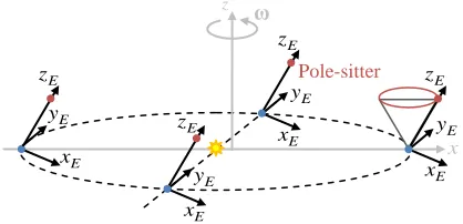
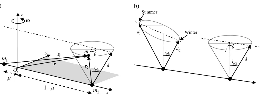
gravitational influence of the small mass on the larger masses is neglected and the larger masses are assumed to move in circular orbits about their centre of mass. Fig. 1a shows the reference frame that is employed. The origin coincides with the centre of mass of the system, the x axis connects the larger masses and points in the direction of the smaller of the two, m2, and the z axis is directed perpendicular
to the plane in which the two larger masses move. The y axis completes the right handed reference frame. Finally, the frame rotates at constant angular velocity, ω, about the z axis, ω=ωzˆ. Also, new units are introduced. The sum of the two larger masses is taken as the unit of mass, i.e. m1+m2=1. Then, with the mass ratio µ =m2
(
m1+m2)
, the masses of the large bodies become m1= −1 µ and m2 =µ (with5
0.30404 10
µ= ⋅ − for the Earth-Sun system). As unit of length the distance between the main bodies is
selected and 1ω is chosen as unit of time, causing ω =1.
Using this reference system, the motion of the pole-sitter spacecraft is described by:
2 U
+ × = −∇ +
r ω r a
(1)
(
)
(
2 2)
1 2
1 / / / 2
U= − −µ r −µ r − x +y with 1
[
]
T
x µ y z
= +
r and 2
(
1)
T
x µ y z
= − −
r . Finally, in Eq.
(1) a represents a thrust-induced acceleration.
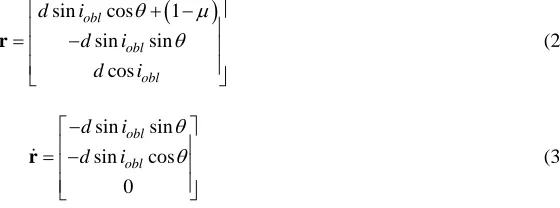
Due to the obliquity of the ecliptic and the rotation of the reference frame, the apparent motion of the Earth’s polar axis describes a cone as depicted in Fig. 1a. The pole-sitter spacecraft needs to track this (clockwise) motion of the polar axis by applying the aforementioned thrust-induced acceleration. The position, r, and velocity, r, of the spacecraft at any time, t, during the year are therefore defined by:
(
)
sin cos 1 sin sin cos obl obl obl d i d i d i θ µ θ + − = − r (2) sin sin sin cos 0 obl obl d i d i θ θ − = −
r (3)
with iobl =23.5° the obliquity of the ecliptic and θ ω= t the instantaneous angular position of the spacecraft along the pole-sitter orbit with θ =0 at winter solstice and θ π= at summer solstice. Note that Fig. 1a and Eqs. (2) and (3) only consider pole-sitter orbits where the spacecraft remains at a constant distance, d, from the Earth (hence the zero velocity in z direction). However, also variable altitude pole-sitter orbits that are more fuel optimal than constant altitude pole-pole-sitters will be considered, where the spacecraft-Earth distance is allowed to vary during the year according to the following sinusoidal law [11]:
( )
0(
1 0)
1 cos 2
d θ =d + d −d − θ (4)
with d0 and d1 the distance from the Earth at winter and summer solstices, respectively, see Fig. 1b.
When substituting Eq. (4) into Eq. (2), the position vector of the spacecraft in the variable altitude orbit,
var
r , is still given by Eq. (2), but the velocity vector needs to be augmented as:
(
)
var 1 0
sin cos 1
sin sin sin 2 cos obl obl obl i
d d i
i θ θ θ = + − −
r r (5)
In accordance with the work in Ref. [11], this paper will consider d=0.01 AU for the constant altitude pole-sitter and d0=0.01 AU and d1= 0.018 AU for the variable altitude pole-sitter. Finally, for all cases
[image:4.612.241.521.182.286.2]a) b)
Fig. 1 Schematic of pole-sitter orbit and reference frame (a) and constant and variable altitude pole-sitter orbits (b).
3
Trajectory phases
The trajectory from LEO up to insertion into the pole-sitter orbit is modelled by distinguishing between two phases: a launch phase and a transfer phase, see Fig. 2. Note that, for now, the launch phase is assumed to be performed by a Soyuz Fregat upper stage, but will later be replaced by a low-thrust spiral in Section 6. The two phases are linked by requiring that the Fregat launches the spacecraft into a two-body elliptic Keplerian orbit (marking the end of the launch phase) that coincides with the initial state vector of the transfer phase (marking the start of the transfer phase). In this section the models adopted to describe both phases will be discussed.
Fig. 2 Schematic of launch and transfer phases.
3.1Launch phase
Before providing the model used to describe the launch phase, it is noted that the objective is not to provide a detailed and optimal launch strategy, but a simple, though reliable, method to assess the relative efficiency of different transfer trajectories. This implies among others that only non-escape launches are considered, i.e. the eccentricity upon insertion into the transfer phase is less than 1.
To model the launch phase, Ref. [17] is used which provides the Soyuz/ST launch vehicle performance through a set of reference missions, assuming a launch from Baikonur (45.6°N, 63.3°E). Due to
ground-θ
d
obl
i
0
d
obl
i
1
d Winter
Summer
y
z
ω
2
m
1
m
1−µ
µ
m
O
θ
r d
obl
i
2
r 1
r
x
Equatorial plane Polar axis
Pole-sitter
Transfer phase
Launch phase
LEO
1
V
∆
2
V
[image:5.612.189.420.408.574.2]path safety rules and authorized drop-zone locations for expended stages, the first three stages can be launched into four launch azimuths, resulting into four initial parking orbit planes, see Table 1. Any remaining inclination changes can be provided by the Fregat upper stage.
Launch azimuth, deg
Reference orbit inclination, deg
60.7 51.8
34.8 64.9
25.9 70.4
[image:6.612.176.496.443.516.2]-10.9 95.4
Table 1 Authorized launch azimuths and corresponding reference orbit inclinations for a Soyuz launch from Baikonur [18].
A typical non-escape Soyuz launch flight profile is provided by Ref. [17] and can be divided into the following phases. First, the three lower stages and the Fregat upper stage are used to reach a low Earth parking orbit with an altitude of hpark =200 km and one of four reference inclinations as provided in Table 1. Then, a first Fregat burn will put the payload on an intermediate transfer orbit with apogee altitude equal to the final orbit altitude and perigee altitude equal to 200 km. During this burn, the Fregat upper stage can also provide a small change of inclination as needed. Finally, after coasting up to apogee of the intermediate transfer orbit, a second Fregat burn raises the perigee and any remaining inclination change is carried out after which the spacecraft separates from the Fregat upper stage. This description suggests that the Soyuz Fregat upper stage approximates a two-body Hohmann transfer from a low Earth, 200 km circular parking orbit (hereafter simply referred to as ‘parking orbit’) to the final target orbit, where any inclination change is distributed over the first (apogee raise) Fregat burn, ∆V1, and second (perigee raise)
Fregat burn, ∆V2, see also Fig. 2.
When applying this approach to launch a spacecraft into a general elliptical target orbit with inclination target
i and apogee and perigee altitudes hapo and hperi, the following Fregat burns are needed:
(
)
1 E 2 t 2 1 t cos i
e park
V e e f i
R h
µ
∆
∆ = + − + ∆
+ (6)
(
)
(
)
2 2 2 1 1 cos 1
E
t target t target i
e apo
V e e e e f i
R h
µ
∆
∆ = − − − − − − ∆
+ (7)
where µE is the gravitational parameter of the Earth, Re=6378 km is the radius of the Earth and f∆i is the fraction of the total inclination change ∆ =i itarget−ipark provided during the first burn, with 0≤ f∆i≤1. Furthermore, the eccentricity of the intermediate transfer orbit, et, is given by:
2
apo park t
e apo park
h h
e
R h h
− =
+ + (8)
while the eccentricity of the target orbit, etarget, equals:
2
apo peri target
e apo peri
h h
e
R h h
− =
Finally, using the rocket equation, the mass that can be injected into the target orbit (i.e. the spacecraft mass plus adapter/dispenser mass of 100 kg [17]) can be determined from:
(
0)
exp /
F
target park tot sp fregat
m =m −∆V I g −m (10)
with ∆Vtot = ∆ + ∆V1 V2, IspF =330 s the specific impulse of the Fregat upper stage [17], g0 the Earth
gravity constant (9.80665 m/s2), mfregat =1000 kg the mass of the Fregat upper stage [17] and mpark the maximum mass in the parking orbit. This mass includes the mass of the Fregat upper stage, the adapter and the spacecraft and is obtained from extrapolating data in Ref. [17] and is presented in Table 2.
Parking orbit inclination, deg
Maximum mass (Fregat + adapter + spacecraft) in parking orbit, kg
51.8 7185
64.9 6449
70.4 6294
95.4 6275
Table 2 Soyuz launch vehicle performance in 200 km circular parking orbit
A validation of this approach is provided through the graphs in Fig. 3, which show the maximum mass (spacecraft + adapter) that can be launched into a circular (a) or elliptical (b-c) target orbit and the penalty on the launch performance when an inclination change needs to be performed (d). The lines indicate the performance as provided by Ref. [18], while the round markers indicate the performance according to the model in Eqs. (6) to (10). Note that the best fit for Fig. 3d to the data in Ref. [17] was found for f∆i =0.15. From the close resemblance between the two data sets in Fig. 3 it can be concluded that the launch model in Eqs. (6) to (10) is a good approximation of the Soyuz launch performance. It can therefore be applied in the design and optimization of the pole-sitter transfer.
3.2Transfer phase
As depicted in Fig. 2, the transfer phase starts from the target elliptic launch orbit up to insertion into the pole-sitter orbit. The initial condition of the transfer phase therefore equals the Keplerian elements of the target launch orbit, while the final condition satisfies Eqs. (2) to (5). While the launch phase is described using a two-body model, the transfer phase is modelled in the CR3BP using the equations of motion in Eq. (1). Furthermore, the transfer can either be ballistic or be performed using SEP, causing the thrust-induced acceleration vector in Eq. (1) to become:
0 Ballistic
SEP
m
=
a T (11)
with T= Tx Ty TzT the SEP thrust vector in the reference frame of Fig. 1 and m the instantaneous mass of the spacecraft. To compute this mass, the equations of motion have to be augmented with the following equation to account for the mass consumption by the SEP thruster:
0
sp
T m
I g
= −
with Isp =3200 s the specific impulse of the SEP thruster, which is in correspondence with the SEP thruster used for the pole-sitter mission in Ref. [11].
a) b)
[image:8.612.72.535.116.497.2]c) d)
Fig. 3 Comparison of launch vehicle performance (spacecraft + adapter mass) from model (round markers) and from Ref. [17] (solid lines) for circular orbits (a) and elliptical orbits with a perigee altitude of 200 km (b-c) for different inclinations of the initial parking orbit. (d) Penalty for an inclination change
from a 51.8° circular orbit with different altitudes.
4
Ballistic transfer phase
less than 200 km, the results in Fig. 4 are obtained for both constant altitude and variable altitude pole-sitter orbits.
The performance of the different ballistic transfer phases can be assessed by linking the launch phase, as described in Section 3.1, to the start of each ballistic transfer. For this, the initial state vector of the transfer is transformed from the CR3BP reference frame in Fig. 1 to the inertial, Earth fixed, equatorial reference frame E x
(
E,yE,zE)
shown in Fig. 5 and is subsequently transformed to Keplerian elements. With the requirement that the mass at the end of the transfer phase should equal 1000 kg and the fact that the transfer phase is ballistic, the mass at the end of the launch phase, mtarget, should also equal 1000 kg. Using Eqs. (6) to (10), the mass required to be launched into the parking orbit, mpark, can then be computed and is used as performance indicator.a) b)
[image:9.612.71.514.231.639.2]c) d)
Fig. 5 Pole-sitter in CR3BP reference frame (gray) and in inertial, Earth fixed, equatorial reference frame (black).
To minimize this mass, rather than truncating the manifold at the point of closest approach to the Earth, a simple grid search can find the optimum location along the manifold to link the launch phase (i.e. the optimum time spent in the transfer phase, tT) and the optimum initial condition of the integration, i.e. the point where the transfer phase winds onto the pole-sitter orbit, θ. The decision vector thus equals
[
tT θ]
=x . For the grid search, bounds of 25≤tL ≤42 days (constant altitude pole-sitter), 25≤tL≤75 days (variable altitude pole-sitter) and 0≤ ≤θ 2π are used and step sizes of ∆ =tT 0.1 days and ∆ =θ 0.01π are chosen. These step sizes are considered small enough to capture the optimal solution. Note that, in case the altitude in the transfer phase becomes less than 200 km or if the eccentricity of the initial state vector is larger than 1, a penalty is introduced on the objective function through a simple if statement. The latter constraint is introduced because the launch model in Section 3.1 can only consider non-escape launches.
The best performing solutions found in the grid search are provided in Fig. 6 and Table 3 for both the constant altitude and the variable altitude pole-sitter orbits and for each of the inclinations of the parking orbit. The results show that, the smaller the inclination of the parking orbit, the larger mpark. This is due to the fact that the inclination of the initial state vector of the ballistic transfer phase is close to 90° (i.e. the pole-sitter position). The launcher thus has to provide the required change between the parking orbit inclination and the inclination of the start of the transfer, which increases for decreasing inclination of the parking orbit and thus penalizes the performance. However, for all inclinations, the results show that a ballistic transfer is feasible using a Soyuz launch, because the mass required in the parking orbit is smaller than the maximum Soyuz performance in Table 2.
Finally, comparing the results for the constant altitude pole-sitter orbit with those for the variable altitude orbit shows only small variations in mpark, but a substantial increase in the transfer time for the variable altitude orbits, because the optimum point of insertion into the pole-sitter orbit lies much farther from the Earth.
z ω
x
E
x
E
z
E
x
E
z
E
x
E
z
E
x
E
z
Pole-sitter
E
y
E
y
E
y
E
a)
park
i =51.8°
b)
park
i =69.4°
c)
park
i =70.4°
d)
park
[image:11.612.74.546.70.290.2]i =95.4°
Fig. 6 Optimum ballistic pole-sitter transfer phases in the dimensionless CR3BP reference frame for constant and variable altitude pole-sitter orbits and for different inclinations of the parking orbit.
Constant altitude pole-sitter Variable altitude pole-sitter Parking orbit
inclination, deg
park
m ,
kg
T
t , days
θ, deg
park
m ,
kg
T
t , days
θ, deg
51.8 5921 34 79.2 5884 63.2 144
64.9 5780 34 79.2 5769 63.2 144
70.4 5736 34 259.2 5736 63.2 144
95.4 5671 34 259.2 5690 47.8 293
Table 3 Minimized mass in 200 km altitude circular parking orbit mpark, transfer phase time tT and location
of insertion into the pole-sitter orbit θ for constant and variable altitude pole-sitter orbits and for
different parking orbit inclinations.
5
Low-thrust transfer phase
In order to improve the performance of the ballistic pole-sitter transfer in terms of mass required in the parking orbit, this section investigates the use of low-thrust propulsion during the transfer phase. For this, the optimal control problem in the transfer phase needs to be solved, while linking the initial state vector of the transfer phase with the launch phase in the objective function.
5.1Optimal control problem
In general, an optimal control problem is to find a state history x( )t ∈nx and a control history u( )t ∈nu, 0, f
t∈ t t , subject to the dynamics:
( )t = ( ( ), ( ), )t t t
x f x u
[image:11.612.85.527.359.456.2](
)
(
)
00, , ,0 ( ), ( ), f
t f f
t
J=ϕ x x t t +
∫
L xt ut t dt (13)and satisfy the constraints c x u( , , )t ≤0. These constraints can include event constraints on the initial and final states and time, bounds on the state variables, control variables and time and path constraints. The first term on the right hand side of Eq. (13) is the endpoint (Mayer-type) cost function, which is only a function of the initial and final states and initial and final time, while the second term is the Lagrange cost function which is a function of time.
To solve the optimal control problem, two different free and open source optimal control solvers are used to compare and validate the individual performances: GPOPS [19] coded in MATLAB® and PSOPT [20] coded in C++. Both implement a direct pseudospectral method to solve the optimal control problem. The time interval is discretized into a finite number of collocation points and Legendre or Chebyshev polynomials are used to approximate and interpolate the time dependent variables at the collocation points. This way, the infinite dimensional optimal control problem is transformed into a finite dimension non-linear programming (NLP) problem. In case of GPOPS the NLP problem is solved using the software package SNOPT (Sequential Non-linear OPTimizer) [21], while PSOPT can make use of either SNOPT or IPOPT (Interior Point OPTimizer) [22].
For the pole-sitter transfer, the state vector, x, is given by the Cartesian position and velocity vectors in the CR3BP reference frame of Fig. 1 and the mass of the spacecraft:
[
x y z x y z m]
=x (14)
while the controls, u, are the Cartesian thrust components in the CR3BP:
x y z
T T T
=
u (15)
Note that the Cartesian thrust components are used rather than two thrust angles and the thrust magnitude as these may give rise to ambiguities [23].
The dynamics of the spacecraft in the SEP pole-sitter transfer are given by Eqs. (1), (11) and (12). Also note that the new units introduced in Section 2 cause the magnitude of the dimensionless mass and thrust to be in the order of 10-18. Therefore, to prevent problems with machine precision and the NLP tolerance, the mass and thrust magnitude are manually scaled back to their physical unites, and are adapted appropriately for use in the equations of motion.
The objective function of the SEP pole-sitter transfer is similar to the objective function of the ballistic transfer, but is written here as a maximization of the total mass fraction, thereby reducing Eq. (13) to:
f park
J= −m m (16)
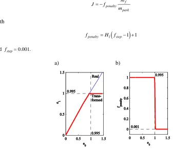
to penalize this objective function value such that the transfer is discarded in the optimization process. The two transformations that are employed are illustrated in Fig. 7. For the transformation of the eccentricity the following step function is used:
(
)
1 1 step 0 0
e =H e −e +e (17)
with e0 the original eccentricity, e1 the transformed eccentricity and H1 a smooth Heaviside function
defined as:
0 1
1
1 tanh 2
step step
e e
H
a
−
= +
(18)
with estep =0.995 and astep= 0.001. Note that the smooth Heaviside function is used to prevent non-differentiable points in the objective function. Then, to penalize the objective function value, Eq. (16) is modified into:
f penalty
park
m
J f
m
= − (19)
with
(
)
1 1 1
penalty step
f =H f − + (20)
and fstep= 0.001.
[image:13.612.82.454.294.584.2]a) b)
Fig. 7 Transformed eccentricity (a) and corresponding penalty on objective function (b) to enable use of launch model for escape orbits.
Finally, three different types of constraints can be distinguished for the SEP pole-sitter transfer, including bounds on the states, controls and time, event constraints and path constraints. The most important bounds are the bounds on the final time and the bounds on the components of the control vector. The final time is free, although a maximum transfer time of 2 years is allowed. The bounds on the control vector are set as follows:
[
max max max]
[
max max max]
T T
T T T T T T
with Tmax =0.25 N the maximum thrust magnitude. The value of 0.25 N is chosen such that the thrust magnitude would be large enough to enable the pole-sitter orbits presented in Ref. [11]. Note that, by allowing the thrust magnitude to vary while previously a constant specific impulse of 3200 s was defined, the assumption is made that thrust magnitude throttling is possible without penalizing the specific impulse. Considering the events, the state vector at the end of the SEP transfer should fully coincide with the pole-sitter orbit conditions provided in Eqs. (2) to (5) . Furthermore, although the penalty on the objective function should already guide the final optimal solution to an eccentricity smaller than 1, an event is included to ensure this:
0 max 0
e −e ≤ (22)
with e0 the eccentricity at the start of the transfer phase and emax =0.995 the maximum allowable
eccentricity. A final event is included to prevent numerical problems with the automatic differentiation used by GPOPS and PSOPT. The numerical difficulties arise when the perigee of the target launch orbit coincides with the parking orbit. Then, the second Fregat burn, ∆V2, becomes zero, its derivative infinite and the optimal control solver exits with an error. Therefore, the following constraint is taken into account to ensure that the perigee of the target launch orbit and the parking orbit do not coincide:
0(1 0) p,min 0
a −e −r ≥ (23)
with a0 the semi-major axis at the start of the transfer phase and rp,min the minimum required perigee
radius, which is set to 6628 km, i.e. 50 km above the parking orbit. Finally, because the Cartesian thrust components are used as control vector, a path constraint needs to be included to limit the total thrust magnitude to Tmax along the whole trajectory,
2 2 2
max
x y z
T +T +T ≤T .
5.2Results
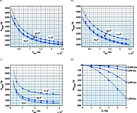
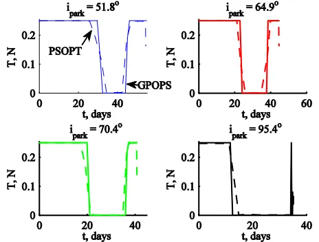
Using the results for the ballistic transfers in Section 4 as initial guess, the results in Fig. 8 and the top part of Table 4 are generated for the constant altitude pole-sitter orbit. Only the results obtained with GPOPS are included since GPOPS and PSOPT provided very similar results, both in terms of the mass required in the parking orbit, the transfer trajectories and the thrust profiles. This is shown in Fig. 9 for the optimized thrust profiles.
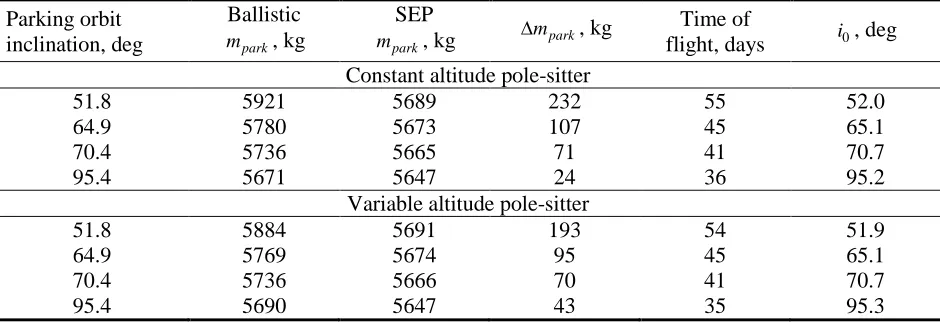
Comparing the results for the SEP transfers with the results of the ballistic transfer (which are included in Table 4 for comparison) shows a decrease in the mass required in the parking orbit of 24 kg to 232 kg, depending on the inclination of the parking orbit. These mass savings can be attributed to the fact that, rather than the Fregat upper stage having to perform the inclination change between the parking orbit and the pole-sitter orbit, the SEP thruster can much more efficiently perform this inclination change. This explanation can be underlined by the value of the inclination at the start of the transfer phase, i0, see
Table 4, which very closely matches the inclination of the parking orbit.
a) b)
c)
[image:15.612.75.528.70.450.2]d)
Fig. 8 Constant altitude pole-sitter: optimized SEP transfer phase in the dimensionless CR3BP reference frame including the SEP thrust vector (a) and in an inertial, Earth fixed, equatorial reference frame (including the launch phase) (b), and the thrust (c) and mass (d) profiles for each value of the parking orbit inclination.
[image:15.612.198.430.509.685.2]a) b)
[image:16.612.67.537.62.455.2]c) d)
Fig. 10 Variable altitude pole-sitter: optimized SEP transfer phase in the dimensionless CR3BP reference frame including the SEP thrust vector (a) and in an inertial, Earth fixed, equatorial reference frame (including the launch phase) (b), and the thrust (c) and mass (d) profiles for each value of the parking orbit inclination.
Parking orbit inclination, deg
Ballistic park
m , kg
SEP park
m , kg ∆mpark, kg Time of
flight, days i0, deg Constant altitude pole-sitter
51.8 5921 5689 232 55 52.0
64.9 5780 5673 107 45 65.1
70.4 5736 5665 71 41 70.7
95.4 5671 5647 24 36 95.2
Variable altitude pole-sitter
51.8 5884 5691 193 54 51.9
64.9 5769 5674 95 45 65.1
70.4 5736 5666 70 41 70.7
95.4 5690 5647 43 35 95.3
Table 4 Constant altitude and variable altitude pole-sitters: comparison of minimized mass in 200 km altitude
circular parking orbit mpark for the ballistic and SEP transfer phases, time of flight in transfer phase
T
[image:16.612.72.542.505.666.2]6
Low-thrust launch phase
[image:17.612.172.404.193.360.2]In order to obtain a full low-thrust trajectory from low Earth orbit to the pole-sitter orbit, this section replaces the Fregat launch phase with a low-thrust spiral, see Fig. 11. To model the low-thrust spiral, it is assumed that the transfer phase as provided in Fig. 8a and Fig. 10a for the constant and variable altitude pole-sitters, respectively, remains unchanged. The problem then becomes to find the thrust profile in each revolution of the spiral such that the spiral starts from the parking orbit and that the end of the spiral coincides with the start of the transfer phase. Furthermore, with the spiral expected to take many months, up to more than a year, the objective is to minimize the time spent in the spiral.
Fig. 11 Schematic of low-thrust launch spiral.
To this end, a locally optimal control profile, similarly to what has been suggested by Gao [16], is applied. This profile consists of the following three steering laws in each revolution of the spiral, which are illustrated in Fig. 12:
- To change the semi-major axis, a tangential steering law is applied around perigee over an angle 2psπ. - To change the eccentricity, a so-called inertial steering law is used where the spacecraft thrusts
perpendicular to the line of apsis around apogee over an angle 2peπ.
- To change the inclination, an out-of-plane steering law is applied around the nodal crossings over an angle piπ , with opposite thrusting direction along the ascending and descending nodes. Note that this steering law is a simplification of the approach suggested in Ref. [16], resulting in a slightly underperforming steering law. However, this simplification is assumed to be allowed because the required inclination changes are only minimal (a maximum of 0.3°, see Table 4).
The controls in each revolution of the spiral thus include the thrust magnitudes of the in-plane, fin ≥0, and out-of-plane, fout ≥0, thrust accelerations and the parameters − ≤1 ps ≤1, − ≤1 pe≤1 and − ≤1 pi≤1 that represent the fraction of the orbit around perigee, apogee and the nodal line where one of three controls is applied. Note that positive and negative values for these three parameters indicate an increase and decrease in the corresponding orbital element, respectively.
Equatorial plane Polar axis
Pole-sitter
Transfer phase
Fig. 12 Illustration of the launch spiral control profile.
To investigate the influence of different control profiles on the launch spiral through an integration of the full set of equations of motion would require a huge computational effort. Therefore, the orbital averaging technique is used, which approximates the equations of motion by calculating the change in the orbital elements after each revolution and dividing it by the orbital period. For the launch spiral, this change in the orbital elements can be computed when starting from Gauss’ variational equations [24] in terms of the eccentric anomaly, E:
(
)
(
)
(
)
(
)
(
)
3 2 22 2 2
2 2 2 2 2 2 sin 1
1 sin 2 cos cos 1
E
cos cos cos
sin sin 1 cos 1
1 cos sin cos sin
cos sin sin 1 cos r C r C n C n C C da a
f e E f e
dE
de a
f e E f E e e E e
d
di a E e
f E e E
dE e
e E
d a E e
f E
dE e i
d d a
i
dE dE e
θ
θ
µ
µ
ω ω ω
µ
ω ω ω
µ ω µ = + − = − + − − − − = − − − −
Ω= − +
−
Ω
= − −
(
)
2(
2)
cos 1 2 cos sin
r
f E e e fθ e e E E
− − − − −
(24)
with a, e, i, Ω and ω the standard Keplerian elements and µC the gravitational parameter of the central body. Note that Eq. (24) holds under the assumption that the thrust acceleration is much smaller than the gravitational acceleration. Depending on the steering law applied, the acceleration components in radial, fr, transverse, fθ, and normal, fn, direction in Eq. (24) are given by:
2 2
2 2 2
2
sin / 1 cos 1 / 1 cos
0 Tangential
sin 1 cos
0 Inertial
1 cos 1 cos E
Out-of-plane
0 0
in
in
r in in n
out
f e E e E f e e E
E e E e
f f f f f
e E e
f θ − − − − − = = = − − (25)
Substituting Eq. (25) into Eq. (24) and integrating over the eccentric anomalies where the separate steering laws are applied, provides the change in orbital elements after one revolution. Note that during this integration the orbital elements are assumed to be constant. Subsequently dividing by 2π gives the sought
out f s pπ e pπ 1 2 piπ
for approximation of the equations of motion. Because the full derivation has been performed by Gao [16], here only the result is provided:
( )
(
)
( ) ( )[
]
(
)
( )[
]
, , ,0 ,0 , , ,0 ,0 3 32 2 2
2 2
2 2 2
2
1 2 2
sign 1 1 1 0.5 0.25sin 2 sign 1 sin
2
1 2 1
1 sign 0.5 0.25sin 2 ln sin 1 cos
2 1 s f e f e s s f s f s s E E
in s in e E
E
C C
E E
in s E
C E
da a a
f p e E e E E f p e E
dE
de a e
e f p E E E e E
dE e e c e
π µ µ
π µ = − + − − − + − − = − + + + − − ( )
[
]
( )(
)
( ) , ,0 , ,0 2 2 2 2 2 2 1 2sign 1 1.5 2 sin 0.25sin 2
1 cos sin 1.5 cos 0.25 cos sin 2 1
sign sin cos 0.25 sin cos 2
2 1 1 1 sign 2 sin e f e
n fi
ni
E
in e E
C E out i C i E out i C a
f p e E e E E
e E eE e E
di a
f p E e E
dE e
d a
f p
dE i
µ
ω ω ω
ω ω π µ π µ = + − − + + − − = + − − + Ω=
∑
(
)
( ) ( ) ( )[
]
, ,0 , , ,0 ,0 2 2 2 1 2 22 2 2 1
2
sin sin 1.5 sin 0.25 sin sin 2
cos cos 0.25 cos cos 2 1
1 2
1 sign 1 cos sin cos sign 0.25 cos 2 cos co
2
n fi
ni s f e f e s E i E E E
in s in e E
E C
e E eE e E
E e E
e
d a a
e f p e E e E f p E e E
dE e e
ω ω ω
ω ω
ω
π µ µ
= − − − − + − − − = − − + + − −
∑
sid dE
Ω (26)
The summation is included to account for the out-of-plane thrust arcs around both nodal crossings and the subscripts ‘0’ and ‘f ’ indicate the initial and final value of the eccentricities Es, Ee and
i n
E during which the tangential, inertial and out-of-plane steering laws occur, respectively. Note that Eq. (26) includes the approximation of two elliptic integrals, which appeared to be accurate for c=0.8 [16]. Finally, the change in mass is given by:
(
)
(
(
)
)
(
)
(
)
, , ,0 ,0
0
, , ,0 ,0
2
, , ,0 ,0
0 1 1 1 sin sin 2 sin sin 1 1 sin sin
2 i i i i
in
s f s f s s
sp
e f e f e e
out
n f n f n n
sp i
mf dm
E e E E e E
dE I g n
E e E E e E
mf
E e E E e E
I g n
π π = = − − − − + − − − −
∑
− − − (27)which leads to a slightly conservative approach as the in-plane and out-of-plane thrust components are not combined into one single thrust component.
Finally, note that the dynamics in Eq. (26) neglect any perturbation on the low-thrust spiral. However, it can be expected that the J2 effect and shadowing have a significant influence on the spiral at low
altitudes, while third body perturbations from the Sun will have a considerable effect at larger altitudes. The latter could be taken into account by considering the Sun‘s gravity perturbation to be constant over one orbit since its period is significantly greater than the period of the spacecraft’s orbit [25]. Alternatively, a double averaging technique could be employed where the second averaging takes place over the period of the Sun [26]. Also, it can be expected that, starting from LEO, the spacecraft spends many revolutions at low altitudes and therefore inside the radiation belts. For future research, it could therefore be interesting to investigate the possibility to use the Fregat upper stage to first raise the orbital altitude above the radiation belts and subsequently initiate the spiral.
6.1Optimal control problem
approach defined in the previous subsections is implemented in PSOPT. The state variables, x, are the first five orbital elements in the inertial, Earth fixed equatorial reference frame of Fig. 5 and the spacecraft mass:
[
a e i ω m]
= Ω
x (28)
The initial and final state vectors are given by the parking orbit and the initial state vector of the optimized transfer phase of Section 6.2, which is indicated by the subscript ‘T, 0’:
0=Re+hpark 0.01 ipark Ωpark ωpark mpark
x (29)
,0 ,0 ,0 ,0 ,0 ,0
f =aT eT iT ΩT ωT mT
x (30)
with the ascending node, argument of perigee and mass in the parking orbit free. Note that the eccentricity of the parking orbit is increased from zero to 0.01 in order for the fifth equation in Eq. (26) to hold, as it approaches a singularity for e=0 [27]. A future change to modified equinoctial elements could circumvent this problem [15, 28].
The controls are the parameters indicating the size of the thrust arc for each steering law and the in-plane and out-of-plane thrust magnitudes:
s e i in out
p p p T T
=
u (31)
Note that PSOPT thus translates a very large optimization problem with the number of static parameters as much as 5 times (i.e. the number of controls) the number of revolutions into a problem where the number of variables are only 5 times the number of collocation points and reinterpolation is used to obtain the control vector in the other revolutions.
The equations of motion are given by Eq. (26). Note that the independent variable of the optimal control problem is the eccentric anomaly rather than what is commonly used, i.e. the time variable. This is done, because PSOPT uses a Lagrange-Gauss-Lobatto distribution to discretize the interval of the independent variable, which results in a larger concentration of nodes at the start and end of that interval. With the orbital period in the last few revolutions expected to be very long, choosing time as the independent variable could give rise to multiple nodes per revolution. Theoretically this means that the control profile can change over these last few nodes, leading to different steering laws, and consequently different equations of motion, within the same revolution. When using the eccentric anomaly as time variable, this problem does not occur since each revolution of the spiral takes an equal portion of the independent variable interval and with hundreds of spiral revolutions, the chance of multiple nodes in the last few spiral revolutions becomes negligible.
Finally, the following path constraints are included: 1 s e
p + p ≤ (32)
2 2
max
in out
T +T ≤T (33)
A trial and error method is employed to generate initial guesses that closely match the boundary constraints and are used to initialize the optimal control solver. Considering the fact that the inclination of the parking orbit is very close to the inclination at the start of the transfer, two dimensional initial guesses suffice. 6.2Results
Results for the low-thrust spiral are shown in Table 5 and detailed results are provided in Fig. 13 for the transfer to the constant altitude pole-sitter and for a parking orbit inclination of 95.4°. The results show a dramatic decrease in the mass required in the parking orbit when the low-thrust spiral, rather than the Fregat launch, is employed: on average 4373 kg. This could allow for a significant reduction in mission cost through the use of a dual launch or even a smaller launcher. However, this comes at an equally dramatic increase in the time of flight. Considering a Hohmann transfer time for the Fregat launch results in launch phase times of approximately 36 days, which increases to an average of 471 days for the low-thrust spiral. The reason for this is the fact that over 1800 revolutions are made, most of them in low Earth orbit, until enough altitude is gained to make the required substantial changes to the orbital elements. As already indicated before, many revolutions at low altitude imply that the spacecraft might spent a large part of the time in the shadow of the Earth. In theory, during this time no power can be generated for the SEP thruster and therefore no thrust force can be generated. An initial investigation into the eclipse time showed that, for the transfer from the 51.8° LEO, the total time spent in eclipse is 32 days, i.e. 7 percent of the total transfer time. This is a significant portion and will have to be considered in future research. Note that a way to reduce the transfer time in the spiral could be by clustering multiple SEP thrusters to obtain a larger maximum thrust. For instance, by adding one SEP thruster (increasing the maximum thrust magnitude to 0.5 N) the transfer time in the spiral can be halved without a penalty on the mass required in the parking orbit.
Finally, Table 5 shows that, because the initial conditions for the transfer phase do not differ much for the constant and variable altitude pole-sitter orbits (provided that the parking orbit inclination is the same), also very similar results are obtained for the optimized spirals for both types of pole-sitter orbits.
Constant altitude pole-sitter Variable altitude pole-sitter Parking orbit
inclination, deg
park
m , kg tsp, days mpark, kg tsp, days
51.8 1308 470 1308 472
64.9 1301 467 1298 475
70.4 1295 469 1294 472
[image:21.612.116.491.455.559.2]95.4 1285 473 1287 469
Table 5 Low-thrust launch: mass in 200 km altitude circular parking orbit, mpark, and minimized time spent
in spiral, tsp, for constant and variable altitude pole-sitter orbits and for each value of the parking
a) b)
[image:22.612.97.539.70.440.2]c)
Fig. 13 Optimized launch spiral (in blue) and transfer phase (in red) (a) and state (b) and control (c) profiles
for a transfer to the constant altitude pole-sitter and for a parking orbit inclination of 95.4°.
6.3Reintegration
elements as needed. The optimization thus loops over the last few revolutions and aims to find in each revolution the magnitude of the in-plane and out-of-plane thrust magnitudes to minimize a weighted sum of the error of the Keplerian elements with respect to the nominal Keplerian elements (i.e. the optimized result from PSOPT).
The results of the reoptimization are added to the results in Fig. 14 and show that, within a maximum thrust magnitude of 0.25 N, the result of PSOPT can be reproduced and the end of the spiral coincides with the initial state vector of the transfer phase. This indicates that, using the full set of equations of motion, the boundary conditions as imposed on the low-thrust launch spiral can be met.
[image:23.612.78.529.192.441.2]a) b)
Fig. 14 Reoptimized integrated solution to match the result from PSOPT for the transfer to the constant
altitude pole-sitter orbit and for a parking orbit inclination of 95.4°. a) States. b) In-plane and
out-of-plane thrust components.
7
Conclusions
mass required in the low Earth parking orbit for a 1000 kg spacecraft to be inserted into the pole-sitter orbit.
When using a Fregat launch phase, masses of 5671 to 5921 kg and 5647 to 5691 kg are required in the parking orbit for the ballistic and SEP cases, respectively. The range in masses is introduced by considering different inclinations for the parking orbit, where the smallest mass is obtained for the inclination closest to 90° (i.e. the pole-sitter position). Mass savings of 24 kg to 232 kg can thus be achieved by using an SEP instead of a ballistic transfer phase. However, both cases are feasible as the mass required in the parking orbit is less than the maximum launcher performance. Comparing the performances for the constant and variable altitude pole-sitter orbits showed only minor differences. With the transfer phase for the variable altitude orbit always entering the pole-sitter at winter (i.e. at the closest distance to Earth), it could be concluded that the altitude of the pole-sitter orbit has a greater influence on the performance than the time of year at which the spacecraft is injected into the pole-sitter orbit, leading to a flexible launch window for the constant altitude pole-sitter transfer. Finally, assuming the transfer phase fixed, the Fregat launch was replaced by a time-optimum low-thrust SEP spiral for which the optimal control problem was solved using a direct pseudospectral optimal control solver. This allowed for another dramatic decrease in the mass required in the parking orbit, but at the cost of an increased time of flight: the mass was reduced to 1285 to 1308 kg, while the duration of the launch phase was increased from 36 to 471 days.
8
Acknowledgements
This work was funded by the European Research Council Advanced Investigator Grant - 227571: Visionary Space Systems: Orbital Dynamics at Extremes of Spacecraft Length-Scale.
9
References
[1] P. Anderson, M. Macdonald, Extension of the Molniya Orbit Using Low-Thrust Propulsion, New Orleans, USA, 2011.
[2] J. Driver, Analysis of an Arctic Polesitter, Journal of Spacecraft and Rockets, 17 (1980) 263-269.
[3] M.A. Lazzara, A. Coletti, B.L. Diedrich, The possibilities of polar meteorology, environmental remote sensing, communications and space weather applications from Artificial Lagrange Orbit, Advances in Space Research, 48 (2011) 1880-1889.
[4] C.R. McInnes, Dynamics, Stability, and Control of Displaced Non-Keplerian Orbits, Journal of Guidance, Control, and Dynamics, 21 (1998) 799-805.
[5] R.J. McKay, M. Macdonald, J. Biggs, C. McInnes, Highly Non-Keplerian Orbits With Low-Thrust Propulsion, Journal of Guidance, Control, and Dynamics, 34 (2011).
[6] C.R. McInnes, The Existence And Stability Of Families Of Displaced Two-Body Orbits, Celestial Mechanics and Dynamical Astronomy, 67 (1997) 167-180.
[7] J. Heiligers, M. Ceriotti, C.R. McInnes, J.D. Biggs, Displaced Geostationary Orbit Design Using Hybrid Sail Propulsion, Journal of Guidance, Control, and Dynamics, 34 (2011) 1852-1866.
[8] J. Simo, C.R. McInnes, Solar Sail Orbits at the Earth-Moon Libration Points, Communications in Nonlinear Science and Numerical Simulation, 14 (2009) 4191-4196.
[9] D.J. Grebow, M.T. Ozimek, K.C. Howell, Advanced Modeling of Optimal Low-Thrust Lunar Pole-Sitter Trajectories, Acta Astronautica, 67 (2010) 991-1001.
[10] R.L. Forward, Statite: A spacecraft that does not orbit, Journal of Spacecraft and Rockets, 28 (1991) 606-611. [11] M. Ceriotti, C.R. McInnes, Generation of Optimal Trajectories for Earth Hybrid Pole Sitters, Journal of Guidance, Control, and Dynamics, 34 (2011) 847-859.
[13] O.M. Golan, J.V. Breakwell, Low Thrust Power-Limited Transfer For A Pole Squatter, American Institute of Aeronautics and Astronautics, Minneapolis, USA, 1988, pp. 717-722.
[14] M. Macdonald, C.R. McInnes, Solar Sail Mission Applications and Future Advancement, New York, USA, 2010.
[15] C.A. Kluever, S.R. Oleson, Direct Approach for Computing near-Optimal Low-Thrust Earth-Orbit Transfers, Journal of Spacecraft and Rockets, 35 (1998) 509-515.
[16] Y. Gao, Near-Optimal Very Low-Thrust Earth-Orbit Transfers and Guidance Schemes, Journal of Guidance, Control, and Dynamics, 30 (2007) 529-539.
[17] T.S.C. Starsem, Soyuz User's Manual (ST-GTD-SUM-01 - issue 3 - revision 0), 2001.
[18] Starsem, "The Soyuz Company", Soyuz User's Manual (ST-GTD-SUM-01 - issue 3 - revision 0), 2001.
[19] A.V. Rao, D.A. Benson, C.L. Darby, M.A. Patterson, C. Francolin, I. Sanders, G.T. Huntington, Algorithm 902: GPOPS, A MATLAB Software for Solving Multiple-Phase Optimal Control Problems Using The Gauss Pseudospectral Method, ACM Transactions on Mathematical Software, 37 (2010) 1-39.
[20] V.M. Becerra, Solving complex optimal control problems at no cost with PSOPT, Yokohama, Japan, 2010, pp. 1391-1396.
[21] P.E. Gill, W. Murray, M.A. Saunders, SNOPT: An SQP Alghorithm for Large-Scale Constrained Optimization, SIAM Journal on Optimization, 12 (2002) 979-1006.
[22] A. Wächter, L.T. Biegler, On the implementation of an interior-point filter line-search algorithm for large-scale nonlinear programming, Mathematical Programming, 106 (2006) 25-57.
[23] J.T. Betts, Practical Methods for Optimal Control Using Nonlinear Programming, Society for Industrial and Applied Mathematics (SIAM), Philadelphia, USA, 2001.
[24] R.H. Battin, An Introduction to the Mathematics and Methods of Astrodynamics, Revised Edition, American Institute of Aeronautics and Astronautics, Inc., Reston, USA, 1999.
[25] T.A. Ely, Mean Element Propagations using Numerical Averaging AAS 09-440, Pittsburgh, Pennsylvania, 2009.
[26] A.F.B.A. Prado, Third-body Perturbation in Orbits Around Natural Satellites, Journal of Guidance, Control, and Dynamics, 26 (2003) 34-40.
[27] J.A. Kechichian, Orbit Raising with Low-Thrust Tangential Acceleration in Presence of Earth Shadow, Journal of Spacecraft and Rockets, 35 (1998) 516-525.
[28] J.T. Betts, S.O. Erb, Optimal Low Thrust Trajectories to the Moon, SIAM J. Applied Dynamical Systems, 2 (2003) 144-170.
Biographies
Jeannette Heiligers
Jeannette Heiligers is a Ph.D. candidate at the Advanced Space Concepts Laboratory at the University of Strathclyde. She obtained her M.Sc. cum laude in Aerospace Engineering from Delft University of Technology, the Netherlands. During her Master she participated in the mission analysis for the European Student Moon Orbiter mission of the European Space Agency at the Department of Aerospace Engineering of the University of Glasgow and her thesis covered the multi-objective optimization of both high- and low-thrust trajectories for an asteroid sample return mission. Funded by the European Research Council, the PhD currently focuses on the orbital dynamics of non-Keplerian orbits using hybrid solar sail and solar electric propulsion and the optimization of transfers to and between non-Keplerian orbits.
Matteo Ceriotti
Colin McInnes
Colin McInnes is Director of the Advanced Space Concepts Laboratory at the University of Strathclyde. His work spans highly non-Keplerian orbits, orbital dynamics and mission applications for solar sails, spacecraft control using artificial potential field methods and is reported in over 100 journal papers. Recent work is exploring new approaches to spacecraft orbital dynamics at extremes of spacecraft length-scale to underpin future space-derived products and services. McInnes has been the recipient of awards including the Royal Aeronautical Society Pardoe Space Award (2000), the Ackroyd Stuart Propulsion Prize (2003) and a Leonov medal by the International Association of Space Explorers (2007).
![Table 1 Authorized launch azimuths and corresponding reference orbit inclinations for a Soyuz launch from Baikonur [18]](https://thumb-us.123doks.com/thumbv2/123dok_us/1674634.120928/6.612.176.496.443.516/table-authorized-launch-azimuths-corresponding-reference-inclinations-baikonur.webp)