Asset protection in a limited swarm environment utilizing artificial potential fields

(1)

Rochester Institute of Technology

RIT Scholar Works

Theses Thesis/Dissertation Collections

2-1-2010

Asset protection in a limited swarm environment

utilizing artificial potential fields

Dieter Laskowski

Follow this and additional works at:http://scholarworks.rit.edu/theses

Recommended Citation

(2)

Asset Protection in a Limited Swarm

Environment Utilizing Artificial Potential Fields

by

Dieter Laskowski

A Thesis Submitted in Partial Fulfillment of the Requirements for the Degree of Master of Science

in Computer Engineering

Supervised by

Associate Professor Dr. Shanchieh Jay Yang Department of Computer Engineering

Kate Gleason College of Engineering Rochester Institute of Technology

Rochester, New York February 2010

Approved by:

Dr. Shanchieh Jay Yang, Associate Professor

Thesis Advisor, Department of Computer Engineering

Dr. Marcin Lukowiak, Assistant Professor

Committee Member, Department of Computer Engineering

Dr. Roy S. Czernikowski, Professor

(3)

Thesis Release Permission Form

Rochester Institute of Technology Kate Gleason College of Engineering

Title:

Asset Protection in a Limited Swarm Environment Utilizing Artificial Potential Fields

I, Dieter Laskowski, hereby grant permission to the Wallace Memorial Library to re-produce my thesis in whole or part.

Dieter Laskowski

(4)

c

(5)

Dedication

(6)

Acknowledgments

I am grateful for the assistance and guidance offered to me by my committee members, especially Dr. Shanchieh Jay Yang for weathering the long distance thesis meetings and his patience through thick and thin. I’d also like to acknowledge Dr. Marcin Lukowiak and Dr. Roy S. Czernikowski for serving on my committee, and their feedback throughout the latter months of the process.

(7)

Abstract

Asset Protection in a Limited Swarm Environment Utilizing Artificial Potential

Fields

Dieter Laskowski

Supervising Professor: Dr. Shanchieh Jay Yang

Asset protection is a behavior in which a team of robots establishes a formation around

a resource marked as an asset in a hostile environment in order to protect the asset from

threats. The robots are assumed to be homogeneous and run a decentralized control

algo-rithm and possess a repulsive quality to the threats. Previous works in this area have used

centralized control or considered the use of many robots. This work aims at developing an

algorithm that is both decentralized, and able to protect assets using only a few robots.

In order to provide this behavior an algorithm coined the Asset Guarding Intelligent

System (AeGIS), was developed and analyzed. Using AeGIS, each robot will detect an

asset move towards it and form a protective formation around it. AeGIS utilizes Quadratic

Artificial Potential Fields (QAPFs) as the robot’s path planning module. As such the fields

are designed to move the robots into formation, avoid collisions, and in turn protect assets.

AeGIS is tested usingLeviathan — an event-driven simulator designed to test groups

of autonomous swarm robots employing distributed control algorithms. The success rate

of different variations of AeGIS were tested. Additionally, the number of threats, robots

employing AeGIS, and the number and mobility of assets were varied to observe their effect

on the success rate. The simulation results show that with sufficient number of robots, the

assets, static or mobile are well protected against 20 modeled threats. Through these results

(8)

(9)

List of Tables

3.1 Table of Variables and Constants used in Equations . . . 27

4.1 Table of Command Line Arguments for use in theLeviathanSimulator . . . 48

4.2 Table of Accepted Strings for Asset Mobility Algorithms . . . 48

5.1 Physical Parameters of Agents in the Simulator . . . 60

5.2 Environmental Parameters of the Simulator . . . 61

5.3 Algorithmic Parameters of Agents in the Simulator . . . 62

5.4 Node placement success for multiple static assets . . . 72

5.5 Node placement success for multiple assets using the random direction mo-bility algorithm . . . 72

5.6 Percent of assets not compromised at chosen time and the rate at which assets become compromised per algorithm for the period of highest threat arrival as defined in Figure 5.15. . . 78

(13)

List of Figures

1.1 nnodes nearaassets in a 2D field of set dimensions, just astthreats appear on the field. . . 3 1.2 Examples of a repulsive (Figure 1.2a) and an attractive (Figure 1.2b)

po-tential field . . . 7 1.3 Aggregate APF of a goal at (0,0) and an obstacle at (1,0) . . . 8 1.4 A potential field function plotted in 2D in terms of distance (Figure 1.4a),

and that same potential field function used as a radial APF and plotted in 3D (Figure 1.4b) . . . 8 1.5 The box canyon problem exists when a robot may be attracted into a local

minima with no desire to leave. . . 10 1.6 A typical QAPF using the equationP(x) = (x−1)2_{. . . 11}

1.7 A QAPF that has been tuned for a stronger repulsion (steeper slope) than attraction. . . 12 1.8 Purely repulsive APF by only utilizing the repulsive component of the

QAPF by way of a piecewise equation . . . 13

2.1 University of Cassino’s Industrial Automation Laboratory setup . . . 18 2.2 Experimental run of DAEIMI’s NSB behavior used to entrap a tennis ball. . 19 2.3 The same simulation as seen in Figure 2.2 but with a fault induced. . . 20 2.4 Magnitude of the inverse force law usingσ1 = 3.0,σ2 = 0.8,c1 = 20and

c2 = 15. Derived using (2.1) from Reif and Wang [11] . . . 22

2.5 Three different stages in Reif and Wang’s castle guarding scenario [11]. . . 23

3.1 Pat, the potential field assets exert on threats . . . 32 3.2 Pnt, the potential field nodes exert on threats . . . 33 3.3 Ptt, the potential field threats exert on threats. . . 34 3.4 Adequate protection of an asset. Protection using fewer nodes may suffice

for most scenarios. . . 35 3.5 The AeGIS Algorithm Flowchart, including the decision making structure

(14)

3.7 3D Plot ofPan . . . 38 3.8 Pnn, the potential field nodes exert on nodes . . . 38 3.9 Insufficient protection for an asset that allows multiple access points for a

threat to compromise protection . . . 39 3.10 Ptn, the potential field threats exert on nodes . . . 40 3.11 Ptnsuccessfully stopping a threat from compromising the asset from Figure

3.9 . . . 41 3.12 Ptncausing failure in asset protection when asset is otherwise well protected 41 3.13 Nodes including Ptn in their calculations are drawn to the stronger threat

force on one side of the asset, exposing the asset to being compromised by a single threat. . . 42 3.14 Overhead view of the local minima problem caused by two assets in close

proximity . . . 42 3.15 Potential Field for 2 assets separated by 2 meters . . . 43 3.16 The formation of spring laws used to test the effectiveness of spring laws . . 43 3.17 A depiction of how late arrivals in a scenario where neighbors are locked

in tends to be defective. . . 45

4.1 Flowchart depicting simulator lifespan . . . 49 4.2 The three zones of which agents can be created in . . . 51 4.3 The process the simulator goes through during its course of execution . . . 52 4.4 The process that the Locomotion Module follows to determine how far a

robot can move in a given time . . . 56 4.5 A screenshot of the GUI mid-simulation. 20 threats appear as red dots, six

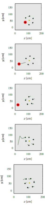
nodes as blue dots and a single asset as a green dot. . . 58

5.1 Success rate for a single static asset under different amounts of threats and nodes . . . 64 5.2 Success rate for a single mobile asset under different amounts of threats

and nodes . . . 65 5.3 Success rate for a single mobile asset choosing intelligent random

move-ments under different amounts of threats and nodes . . . 66 5.4 Cumulative success rate for assets utilizing each mobility algorithm while

varying number of threats and nodes . . . 67 5.5 A depiction of how different mobility models the asset can employ effect

(15)

5.6 Success rate for multiple static assets while varying the number of nodes and threats . . . 69 5.7 Success rate for multiple mobile assets while varying the number of nodes

and threats . . . 70 5.8 Average number of nodes received versus the number of nodes given to

each asset for static assets. . . 71 5.9 Average number of nodes received versus the number of nodes given to

each asset for multiple assets employing the random direction mobility model. 72 5.10 Success rate for multiple static assets while varying the number of nodes

and threats with assets being created simultaneously . . . 73 5.11 Success rate for multiple mobile assets while varying the number of nodes

and threats with assets being created simultaneously . . . 74 5.12 Assets not compromised over simulation time in a field of randomly placed

nodes comparing the basic algorithm to theFtn algorithm. . . 75 5.13 The presence of nodes in formation and the arrival rate of threats from the

simulations in Figure 5.12. . . 76 5.14 Assets not compromised over simulation time in a field of randomly placed

nodes comparing the adaptive algorithm to the basic algorithm and theFtn algorithm. . . 77 5.15 Regions of interest in threat arrival overlaid on a plot of the average number

of threats at the assetversustime. . . 78 5.16 Emergent threat behavior, where the three threats shown push the inner

threat through the asset’s protective formation. Threats typically spread out around the protective formation prior to layering. . . 80

(16)

Chapter 1

Introduction

The term “robot” was first used in Karel Capek’s play,Rossum’s Universal Robotsin 1929

in which the robots were a race of workers created by the play’s inventor, Rossum, from

a vat of biological parts. Capek coined the workers “robots,” a term derived from the

Czech word robota, which is loosely translated as menial laborer [9]. To this end “Rossums

Universal Robots” demonstrated how robots were able to replace “real” people from any

type of labor that was deemed too lowly to merit respect, subsequently freeing humans to

do more meaningful work.

Today robots are still used to replace workers in roles where a robot’s precision, ability

to repeat a task accurately, and their expendability make them more desirable in a role than

a human worker. Robots have been used in applications ranging from robotic welding arms

in production lines, to robotic vacuum cleaners, to bomb defusal and search and rescue

robots.

Some of these robots are considered to be autonomous, which means that they think

and act on their own without human interaction or direction. This level of autonomy opens

up the use of autonomous robots to be left to complete a task unsupervised by humans,

freeing them to perform other tasks as in Capek’s play. Commonly the tasks assigned

to autonomous robots can be accomplished faster through the use of multiple autonomous

robots, other times the task may be impossible without the use of multiple robots. The

(17)

and is described in detail in Section 1.2.

Cooperative robotics may be utilized in a manner that would allow multiple autonomous

robots to perform the tasks previously described that would be too dangerous for human

workers. One of the main motivations for robotics research is the desire to remove humans

from dangerous work and replace them with an expendable robot. One such task is that of

asset protection.

Asset protection, as it sounds, is the protection of resources labeled as assets from harm.

The need for asset protection arises from the presence of a resource in a hostile

environ-ment. This resource is in the hostile environment for any number of reasons, whether the

resource is trapped there, has a particular task to perform within the environment, or simply

needs to traverse the environment in order to deliver supplies, information, or get home. In

any case the resource is valuable to the implementer, so it will be marked as an asset.

Typically the nature of the hostile environment will not be known aside from its

disposi-tion. A hostile environment will have agents that can do harm to the asset; as such they will

be labeled as threats. As the nature of the environment is not usually known beforehand,

the strength, number and location of these threats is unknown to the asset, so it cannot plan

to avoid them. The asset is left defenseless against the threat.

For whatever reason the asset is in the hostile environment it becomes necessary to

have a general, flexible response to threats. This problem is posed generally as the “asset

protection” problem. Assuming that enough is known about the hostile environment that a

number of robots may be equipped that will be able to repel these threats, the robots can be

used to protect the asset from the threats. With this information the problem itself can be

properly formulated.

1.1

Problem Statement

Given an environment in which assets are defined and threats are present, a number of

(18)

[image:18.595.136.483.87.289.2]

Figure 1.1: nnodes nearaassets in a 2D field of set dimensions, just astthreats appear on the field.

effect the nodes have on the threats.

The environment is a 2D field of fixed dimensions that will containaassets,nnodes and

t threats during the course of a simulation. Initiallyn nodes are present in the simulation

and turned on, followed by a assets being defined within the environment, followed by t

threats, alerted to the assets’ presence in the field attempting to compromise the asset.

Multiple threats appear in the environment after the assets are identified and employ

their own path planning algorithm to avoid the nodes and reach the assets. These threats

exploit their knowledge of the environment and have omniscient information about the

locations of the assets and nodes.

Conversely the assets are of singular purpose and pay no heed to efforts or locations of

the nodes in the environment. The assets can either be stationary, as if performing a task at

a location, or mobile, attempting to get from one location to another.

In either case the nodes attempt to form a protective formation around the assets. Ideally

this would consist of many nodes forming a circle coincident on the asset leaving no

en-trance for a threat to get to the asset, but in many cases the resources would not be available

(19)

when there are not enough nodes to form a robust circular formation. For this reason and

the purposes of asset protection, any formation, structure, or behavior of nodes that result

in an asset being protected from a threat will be considered asset protection.

Constructing such behavior on numerous robots of limited capabilities is a non-trivial

matter. The behavior must be able to protect the assets from threats when there are

“suf-ficient nodes” to produce a robust circle formation, but able to alter their formation based

on the number of nodes in formation without communicating with each other. In order

to provide such a behavior Artificial Potential Fields (APFs) are employed to construct an

asset protection behavior that is robust to individual node failure, but simple enough to be

used on robots of limited means. This solution to the asset protection problem is called

the Asset Guarding Intelligent System (AeGIS). Details on the AeGIS algorithm used is

described in Section 3.6 while APF functionality in general can be found in Section 1.3.

1.2

Cooperative Robotics

The concept of cooperative robotics entails a group of robots that work together to achieve

a common goal. Algorithms within the field of cooperative robotics are commonly divided

into two categories; centralized and decentralized.

Centralized robot controllers use a single entity (computer, other robot, etc.) that tells

each robot what to do. A centralized controller is typically chosen for environments in

which the coordination of the robots needs to be carefully orchestrated and knowledge of

the environment is easily attainable. Centralized robot controllers typically have either

global knowledge, or the collective knowledge of each of the robots it controls meaning it

will always have more knowledge than any singular robot would. Using this knowledge

the centralized controller can easily make informed decisions and send the robots accurate

instructions throughout the course of the mission.

Decentralized robot controllers trade optimal knowledge and coordination for system

(20)

from the environment and decide what its next action is on its own. This process of

in-dependent control introduces system wide robustness in the sense that if any robot is

dis-abled, or otherwise rendered ineffective, the system will continue to operate normally with

the exception of the affected robot. In a centralized controller, if the controller is disabled,

or receives bad information, or is unable to transmit instructions, the entire system will be

rendered ineffective. However this trade off typically means that complicated tasks

requir-ing coordination of multiple robots will be much harder to accomplish in the decentralized

controller.

Cooperative robots have been used in a number of scenarios in an effort to remove

hu-mans from menial or dangerous tasks. Some such tasks would be those such as coordinated

group movement of an object [6, 15], escorting a target by surrounding it and maintaining

formation relative to the target’s position [3], and robot soccer [20].

1.3

Artificial Potential Fields

Artificial Potential Fields (APFs) are a simple mathematical path planning algorithm based

on naturally occurring potential such as gravitational potential or electrical potential. APFs

are commonly described using functions for their compactness and computational speed

and are sometimes for this reason called Artificial Potential Functions.

Agents interact with the fields as Newtonian Particles, resulting in them needing to

fol-low Newton’s force laws with respect to gravitational potential. In this manner the potential

fields exert a force upon the particles in the system in the direction of the lowest potential.

In order to determine these forces the force vector is defined as the negative gradient of the

potential field.

⃗

(21)

In order for these forces to be useful as a path planning algorithm the virtual

environ-ment must be shaped in a way that the forces will lead the agent away from obstacles and

ultimately towards its goal. Taking note of this, each object in the environment is given a

potential field, either attractive or repulsive. Significant locations in the environment can

also be given potential fields. Obstacles will be given repulsive potential fields and goals

will be given attractive potential fields.

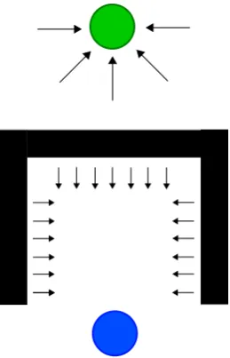
A repulsive potential field can take many shapes, but keying off of the concept of

gravi-tational potential, a repulsive potential field will have a high potential at the origin, tapering

off to lower potentials as distance from the origin increases until the limit of the repulsive

field at which the field would be level with the rest of the environment, producing no force.

An example of such a repulsive potential field can be seen in Figure 1.2a. When the force

gradient is calculated for the repulsive APF, it should point away from the origin of the

field.

An attractive potential field is created in much the same manner as the repulsive

po-tential field. In order to produce an attractive popo-tential field the origin of the field must

be surrounded by rings of successively higher potential so that when the force gradient is

calculated it will point towards the origin of the field. An example of such an attractive

potential field can be seen in Figure 1.2b

Navigation of an environment that contains both goals and obstacles using APFs still

involves calculating the force vector produced by the fields. The environment can be

de-scribed by the collection of all the potential fields in the environment. The fields are

col-lected by calculating an aggregate potential field by summing each of the individual

po-tential fields relative to their position in the environment. From this point the force vector

acting on the agent can be determined by calculating the negative gradient at the agent’s

position in the aggregate potential field.

(22)

-2

0

2

X _-2

0 2 Y 0 2 4 6 Potential

(a) A purely repulsive potential field centered at (0,0)

-2 0 2 X -2 0 2 Y 0 5 10 15 Potential

(b) A purely attractive potential field centered at (0,0)

Figure 1.2: Examples of a repulsive (Figure 1.2a) and an attractive (Figure 1.2b) potential field

Ptotal(x, y) = ∑

n

Pi(x, y) (1.3)

Commonly the APFs are stored as functions in order to reduce the storage required and

speed up computations for potential field values. One of the methods to produce simple

attractive and repulsive potential fields is to describe them using radial potential field

func-tions. In a radial potential field function, the potential field is described by an equation

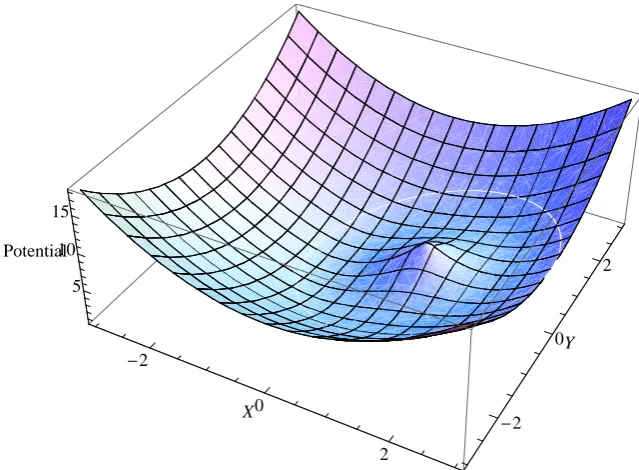
whose only parameter is distance from the origin. One such APF is shown in Figure 1.4.

When using functions to describe APFs, the APFs are centered at the origin, resulting in

the use of localization variables to place the APF within the virtual environment. These

variables are in fact the coordinates of the objects with which the APF is associated.

Ptotal(x, y) = P1(x−x1, y−y1) +P2(x−x2, y−y2) +· · ·+Pn(x−xn, y−yn) (1.4)

In (1.4) the localization variables, xi andyi are the location of each of the objects in

the virtual environment. If the functions are a function of distance from the origin, then

(23)

-2

0

2 X

-2

0 2

Y 5

10 15

Potential

Figure 1.3: Aggregate APF of a goal at (0,0) and an obstacle at (1,0)

0.5 1.0 1.5 2.0 2.5 3.0 Distance

1 2 3 4 5 6 Potential

(a) A plot of a potential field function in terms of distance

-2

0

2

X _-2

0 2

Y

0 2 4 6

Potential

[image:23.595.148.468.121.356.2]

(b) The same potential field function plotted in 3D

(24)

√

(x−xi)2+ (y−yi)2 which results in (1.5), wheredis distance from the origin.

Ptotal(x, y) = P1(

√

(x−xi)2+ (y−yi)2) +P2(

√

(x−xi)2+ (y−yi)2) +. . .

+Pn( √

(x−xi)2+ (y−yi)2)

Ptotal(x, y) = P1(d) +P2(d) +· · ·+Pn(d) (1.5)

NowPtotalcan be expressed as a sum of one variable as in (1.3).

Ptotal(x, y) = ∑

n

Pi(d) (1.6)

Computation of the force vector acting on the agent can be further accelerated by taking

advantage of the aggregate potential field being described as a sum of functions, in which

the aggregate force acting on the agent can be calculated by a single derivative over the

equation describing the aggregate potential field, since the potential field has been reduced

to a single variable of distance from the origin of each field. Additionally, since the field is

radial the force vector will point either towards the origin or away from the origin based on

the polarity of the force.

Fnet(x, y) = d

d(d)(Ptotal(x, y)) (1.7)

The potential field equations can be stored as force equations due to the sum rule of

derivatives.

d

d(d)(Ptotal(x, y)) =

d d(d)

( ∑

n

Pi(d) )

=∑

n (

d

d(d)Pi(d) )

(1.8)

Equation (1.8) results in a compact simple method for calculating the force vector acting

on an agent at any location in the environment. Using this relationship the net force acting

(25)

[image:25.595.245.375.88.290.2]

Figure 1.5: The box canyon problem exists when a robot may be attracted into a local minima with no desire to leave.

from the agent to each object in the environment and summing the force vectors, producing

the direction and magnitude that the agent should move in.

However APFs do have a few notable disadvantages when compared to other path

plan-ning algorithms. Some behaviors may be difficult or almost impossible to describe using

APFs, while complicated behaviors may still take a very long time to design. Another

prob-lem that APFs incur is that of local minima. A local minima in an APF is a point where the

agent has no force vector acting upon it, though a global minima (point of lower potential)

that is more desirable exists elsewhere in the environment. An example of a local minima

is shown in Figure 1.5 as the box canyon scenario. In this scenario the agent is drawn into

the canyon by the goal beyond it. Once the agent is within the box canyon it encounters

the repulsive force of the canyon itself, and since it still sees the goal beyond the canyon it

doesn’t attempt to escape the canyon itself; it is caught in a local minima.

There are however some solutions to the local minima problem, including stream

func-tions [21], introducing an excitation factor or randomness to shake the robot out of the local

(26)

0.5 1.0 1.5 2.0 2.5 3.0 Distance 1

2 3 4 Potential

Figure 1.6: A typical QAPF using the equationP(x) = (x−1)2.

1.3.1 Quadratic Artificial Potential Fields

APFs can take many forms, and the equations describing them can be as complex or as

simple as the implementer desires, however they are often kept simple in order to maintain

the algorithmic nimbility for which they often are utilized.

Quadratic Artificial Potential Fields (QAPFs) demonstrate the two main forces

em-ployed in applications of APFs: attraction and repulsion. A QAPF typically takes the

shape of a parabola in such a manner that it generates short range repulsion and long range

attraction. These fields are useful for purposes where the agent is needed to maintain a

distance, but still stay near to another agent or object. A normal QAPF can be tuned in the

same manner that a parabolic equation can (Figure 1.6).

An additional amount of configuration can be included by making the QAPF a

piece-wise function in which each lobe of the QAPF has its own tuning coefficient, and a common

centering point.

In this manner a QAPF may be tuned to have a stronger repulsive force than attractive

force or however the implementer decides to design it. The force equation is calculated by

taking the derivative of each lobe individually.

(27)

0.5 1.0 1.5 2.0 2.5 3.0 Distance 1

2 3 4 Potential

Figure 1.7: A QAPF that has been tuned for a stronger repulsion (steeper slope) than attraction.

purely repulsive force by negating one of the lobes completely. This is demonstrated in

Figure 1.8 where the field retains only repulsive behavior.

1.4

Swarm Robotics

Swarm intelligence is described as a set of simple behaviors that when followed by each

member of the swarm will produce a group, or emergent behavior. A swarm environment

is most commonly characterized as a decentralized control algorithm employed on

homo-geneous robots that are programmed with relatively simple behaviors that together display

some emergent behavior [4].

Swarm robotics is based on the observation of swarms in nature such as bees, ants and

other creatures. In each one of these swarms, when a single agent is taken out of the swarm

it will exhibit simple individual behavior, when there are many agents however, they act as

a swarm they can accomplish large tasks.

Various species of ants cooperate without direct communication, though modifications

of the environment called stigmergy[6]. Through stigmergy ants cooperate to bring large

prey back to the hive, prey that individually they would not be able to bring back. The

(28)

0.5 1.0 1.5 2.0 2.5 3.0 Distance 0.1

0.2 0.3 0.4 0.5 Potential

Figure 1.8: Purely repulsive APF by only utilizing the repulsive component of the QAPF by way of a piecewise equation

to the prey, and through physical pushing of the prey they eventually decide on a direction

to move.

In a limited swarm environment the number of agents in the system is substantially

smaller than that of a typical swarm. Typical swarms employ between hundred and tens of

thousands of agents. Swarms in robotics typically do not reach this size in experimentation

due to their cost, however they can be achieved in simulation. Swarms in robotics have

been seen as small as 10-20 robots, but a limited swarm environment would have its target

population between 5-20 robots.

1.5

Flocking

One of the most effective forms of formation control observed in nature is a behavior

recog-nized as flocking. Flocking is a method that organisms utilize to avoid predators, increase

survival chances and in some cases even reduce strain on travel.

Flocking as it is known today in computer science circles originated with Reynolds who

was searching for an easy way to generate paths of birds and fish while creating computer

(29)

path for each object in the flock would have to be individually plotted out by the animator.

Now with Reynolds’ rules, only the leader of the flock’s path must be scripted leaving the

rest of the flock mates to “flock.” Reynolds’ rules of flocking follow [12].

1. Collision Avoidance: avoid collisions with nearby flockmates

2. Velocity Matching: attempt to match velocity (a vector quantity) with nearby

flock-mates

3. Flock Centering: attempt to stay close to nearby flockmates

Collision avoidance manifests itself as a short range repulsive force between

flock-mates, and velocity matching is somewhat complimentary. These two behaviors are also

sometimes referred to as static collision avoidance and dynamic collision avoidance. Static

collision avoidance considers only the location of the flockmates, ignoring velocity, which

makes it similar to the collision avoidance behavior seen in APFs, while dynamic collision

avoidance is based only on velocity of flockmates and ignores location. As Reynolds puts

it, “if the [member of the flock] does a good job of matching velocity with its neighbors, it

is unlikely that it will collide with any of them very soon.”

Flock centering is a behavior that makes the member want to be in the middle of the

flock. If a member is deep in the flock, the presence of flock members around it will cause

it to be pulled at roughly the same strength in all directions resulting in a near zero sum

force. But if a flock member is on the outside of a flock, it will be pulled towards the center

of the flock. This behavior can be drawn easily from the protective quality of flocks seen

in nature. It is flock centering that essentially makes the flock a cohesive entity.

These flocking rules are implemented on all flock members besides the leader as a

distributed control algorithm. When each member of the flock adheres to these three rules

the flock appears to be cohesive and act as an entity with a single mind.

Reynolds noted that the flocks seemed to behave more real when the sensing range was

(30)

position in the flock as long as their neighbors do not change, so a flock would be able to

conduct various maneuvers that would respond to obstacles or predators.

It’s not a far stretch to see how Reynolds’ flocking rules can be implemented using APFs

[16, 17]. Additionally flocking can easily be adapted to escorting objects or members of

the flock by having the flock treat the object as a flockmate and the object being controlled

independently.

1.6

Organization of Thesis

The layout of this work is as follows: Chapter 2 goes over works done by other researchers

similar to this problem. Chapter 3 will detail the algorithms used to model asset and threat

behavior, as well as explain in detail the node’s asset protection algorithm, AeGIS. Chapter

4 discusses the architecture of the simulator used to simulate the algorithms described in

Chapter 3. Chapter 5 shows the simulation parameters and the simulation results. Finally

Chapter 6 discusses the conclusions based on the results in Chapter 5 and possible future

(31)

Chapter 2

Related Work

Several strategies have been attempted in order to solve what is commonly described as

the Entrapment/Escorting scenario. Entrapment is the act of robots surrounding an object

preventing its escape by creating a surrounding formation. This formation is also called

a “containment” formation due to its use to “contain” the object to its current location.

Escorting is the act of achieving an entrapment or containment formation, but not using it

to keep the object in place and instead maintain a formation around the object and guiding

it along its path, or protecting it from outside threats.

2.1

Centralized Controller for Entrapment/Escorting

Antonelliet al.’s approach to the entrapment/escorting problem utilizes a centralized

con-troller employing their Null Space Based (NSB) control method to manipulate a multirobot

system to escort an object in both a simulated environment, and a physical one.

The NSB control method attempts to find a move for each robot that will satisfy a

set of subproblems that will be individually solved, and then based on the priority given

to each subproblem combine the solutions into one move. NSB control utilizes a task

Jacobian matrix, commonly utilized in robotic manipulation, to find a “closed-loop inverse

kinematics least-square solution.” Antonelli et al. claim that the NSB control method

“always fulfills” the highest priority task by making sure that none of the solutions to the

(32)

that two solutions do conflict with each other the components of the lower priority tasks

that conflict with the highest priority task are removed from the final move of the robot.

In order for NSB control to be applied to the escorting mission it was broken down into

four subproblems:

1. Command the robots’ centroid to be coincident with the target

2. Move the robots on a given circumference around the centroid

3. Properly distribute the robots along the circumference

4. Avoid collisions among the robots themselves and with obstacles

Antonelliet al. ran several simulations varying the priorities given to these subtasks in

order to see how the NSB controller combined these tasks, and what would be the optimal

priority. The simulations showed that given a satisfactory ordering of the subtasks the

robots were able to converge on the target quickly and accurately.

University of Cassino’s (UNICAS) Industrial Automation Laboratory’s (LAI)

multi-robot setup includes six Khepera II multi-robots with Bluetooth modules and a computer system

that reads the robots’ position on a smooth table via two overhead video cameras. The

computer system consists of a computer running Windows XP that reads the camera

im-ages via frame grabbers and sends the acquired image to a Linux-based PC which runs the

NSB control algorithm and transmits the movement information to the robots (Figure 2.1).

Needless to say this makes the control algorithm centralized.

The experimental results as shown on DAEIMI’s website1 show that NSB control is

both accurate and robust in its ability to deal with robot fault. Additionally the system

appears to react quickly to change in target position (escorting) and maintain a stable

for-mation around the target. For their target in their experiments the robots escort a tennis ball

that is given an impulse by one of the authors in the lab.

1

(33)

Figure 2.1: University of Cassino’s Industrial Automation Laboratory setup (http://webuser.unicas.it/lai/robotica/Laboratory.html).

However the Robotics Research Group at DAEIMI has also experimented with

decen-tralized control schemes and applied them to flocking algorithms as evidenced by the videos

on their website and published papers on flocking [2], however it does not appear that they

have taken to decentralizing their NSB control scheme at this time, though they do express

an interest in doing so.

Another group that has attempted to solve the entrapment/escorting mission utilizing a

centralized controller is Mas et al. who use a “cluster-space” approach which groups the

n-robots of a system as a single entity, and constructing Jacobian and Inverse Jacobian

ma-tricies to find the inverse kinematic solution to place their three degree of freedom robots

at the desired locations [7]. As with Antonelliet al., Maset al.plan to look into

decentral-izing their approach to the entrapment/escorting algorithm in order to reap the benefits of a

(34)

[image:34.595.205.417.142.607.2]

(35)

[image:35.595.258.353.148.587.2]

(36)

2.2

Social Potential Fields

Reif and Wang at Duke University experimented with setting up a framework in which

APFs were used to form relationships between different groups of robots by setting up

different APFs for each group, defining intra- and inter-group behaviors [11]. They hoped

that by setting up this framework that APFs could be designed in a scalable manner so

that they could be applied to Very Large Scale Robotics (VLSR) and be applied to both

industrial and military applications. A VLSR system as described by Reif and Wang would

target between hundreds and tens of thousands of robots.

The social potential field framework is a distributed control mechanism across the

VLSR system of homogeneous robots. These robots are divided up into groups of which

intra-group (within the group) and inter-group (other groups) behavior is defined. Through

this process, groups and relationships are defined that produce the desired behaviors.

Reif and Wang’s approach involved the use of inverse-power laws to define their

poten-tial fields. The inverse-power law is described as being similar to those found in molecular

dynamics, in which a field can exhibit long-range attraction, but short-range repulsion.

Their example inverse-power law characterized by (2.1) embodies both attractive and

re-pulsive forces.

f(r) = −c1

rσ1 +

c2

rσ2

c1, c2 ≥0, σ1 > σ2 >0

(2.1)

In (2.1) the function can be tuned by altering the parametersσ1,σ2,c1andc2. Attraction

is controlled by the termc2/rσ2 while repulsion is controlled by−c1/rσ1. Whenc1, c2 >0,

assuring positive attraction and repulsion forces the inverse-power law becomes a

cluster-ing force law. The strength of the attraction and repulsion can be tuned using σ1 and σ2.

Whenσ1 > σ2 >0the repulsive force will dominate at short distances while the attraction

will have a stronger effect over long distances. The distance at which these forces take

(37)

5 10 15 20Distance

-6

-4

-2

0 2 4 6 8 Force

Figure 2.4: Magnitude of the inverse force law usingσ1 = 3.0,σ2 = 0.8,c1 = 20andc2 = 15.

Derived using (2.1) from Reif and Wang [11]

that repulsion will be strong at short ranges, will decay rapidly with distance, while a small

σ2 will give the attractive force a stronger long range effect.

The process to which these potential fields are designed to function in the social

poten-tial field framework is proposed to be as follows:

1. Specify the required behavior

2. Design intra-group forces

3. Design inter-group forces

4. Define the dynamic element of the potential force laws

Reif and Wang test this approach in several scenarios, from the simple task of clustering

to the relatively complex behavior described as bivouacking. The most relevant scenario

they test is a scenario called “guarding a castle.”

In the “guarding a castle” scenario three groups of robots are defined: the castle, the

guards and the attacker. The castle is represented by a singular “landmark” robot, which

(38)

(a) (b) (c)

Figure 2.5: Three different stages in Reif and Wang’s castle guarding scenario [11]. In Figure 2.5a the initial setup is shown with many “guards” and one landmark robot (circled) that acts as the “castle.” In Figure 2.5b the state of the system is shown after the guards have taken formation around the castle. In Figure 2.5c an attacker (circled) is shown attempting to find vulnerabilities in the castle’s protection, and the guards are seen chasing after the attacker

guards are represented by a number of identical robots and the attacker, or invader consists

of only one robot.

Force laws are defined such that the guards are attracted to the castle, but repelled to

a distance away from it to simulate a perimeter. Additionally the guards are repelled by

each other to spread out the formation and avoid collisions. The guards are attracted to the

attacker, but the attraction is weak enough that the guards tend to stay near the castle. The

attacker is then designed to be attracted to the castle but repelled by the guards.

Reif and Wang observe that this behavior can be achieved without defining complicated

rules that each robot has to follow to achieve the desired result. To this end it is proposed

that many complex behaviors can be implemented by defining multiple groups of robots

and their inter- and intra-group actions.

As an extension, Reif and Wang discuss the application of spring laws in an attempt to

form what they describe as “exact structures.” Hooke’s spring restoration force laws are

applied to robots in such a manner that they will form a predefined formation based on the

number of connections and the strength of the “springs” themselves. This concept of using

(39)

is important to note, as it may be applied to formation control or flocking.

2.3

Threat Containment

Threat containment is a variation of the entrapment problem where the objects to be

en-trapped are threats. In order to pacify the environment, robots actively seek out threats in

the environment to surround, and thus contain the threat’s impact to the rest of the

environ-ment.

Mehendale designed the event driven simulator MAHESHDAS to simulate a swarm

environment in which threats would be created randomly throughout the course of the

simulation and it would be up to a number of robots to surround and contain them [8].

The approach was based on QAPFs that would hold the robots in a radial formation around

the threat, while a special node spreading force would attempt to assure that the nodes were

spread out around the threat in addition to the normal node to node repulsive force.

Ransom also worked on this problem and enhanced the success rate of threat

contain-ment by using ad-hoc wireless networks set up by the robots to control the number of nodes

containing a single threat [10]. Ransom noticed that in some cases the robots would have

a disproportionate number of robots containing a single threat, while other threats in the

environment were not contained, or had inadequate containment. Using wireless networks

the robots could control the number of nodes at a single threat by making robots just

ar-riving to the threat ask for permission to join the containment formation. Additionally the

wireless networks were used to maintain formation by each robot identifying and

com-municating with its neighbors, and Ransom’s Mid-Angle Formation Algorithm (MAFA)

ensuring equal distribution around the threat.

Both Mehendale and Ransom’s algorithms rely on having a superior number of robots to

threats. In both Mehedale and Ransom’s work, the threats were containable, meaning that

there were no difficulties to containing a threat once it was located. Ransom experimented

(40)

(41)

Chapter 3

AeGIS Asset Protection Algorithm

Asset protection itself involves identifying what the assets are in the environment. This

means an asset can take the form of something static (something that does not move) such

as a building or physical location, or something dynamic (something that moves) such as

a convoy or person. The labeling of assets can be done in any environment at the

imple-menter’s discretion, but for the purposes of simulation it will be done by the simulator as

described in Section 4.2.

From this point, asset protection involves forming a protection algorithm to protect the

assets from the threats. The manner in which this is done is highly interdependent on the

capabilities and behaviors of each of the agents, which will be discussed throughout this

chapter.

The asset protection algorithm has gone through many stages of development and

rede-velopment based on incremental testing and analysis of results. In this manner each of the

three agents involved in this algorithm were added and their features tested. This chapter

describes the capabilities and algorithms employed by each of the three agents in the asset

protection scenarios, assets, threats and nodes.

All agents share the following simulator properties. The agents are modeled as a

cir-cular robot in a 2D plane with a fixed radius. Their location, or state, is stored using a

coordinate system that keeps track of their position, (x, y)and orientation,θ. Their

(42)

Table 3.1: Table of Variables and Constants used in Equations

Variable Meaning

Pat Potential Field Assets exert on Threats

Pnt Potential Field Nodes exert on Threats

Pan Potential Field Assets exert on Nodes

Pnn Potential Field Nodes exert on Nodes

Ptn Potential Field Threats exert on Nodes

Ptt Potential Field Threats exert on Threats

αat Coefficient that controls the force ofPat

αrn Coefficient that controls the magnitude of the repulsive component ofPan

αan Coefficient that controls the magnitude of the attractive component ofPan

ηrt Coefficient that controls the magnitude of the repulsive component ofPnt

ηrn Coefficient that controls the magnitude of the repulsive component ofPnn

τrn Coefficient that controls the magnitude of the repulsive component ofPtn

τan Coefficient that controls the magnitude of the attractive component ofPtn

τrt Coefficient that controls the magnitude of the repulsive component ofPtt

dat Distance from Asset to Threat

dnt Distance from Node to Threat

dr Distance from Asset to Node

dnn Distance from Node to Node

dtn Distance from Threat to Node

dtt Distance from Threat to Threat

ddnt The Distance Threats desire to be away from Nodes

ddrn The Distance Nodes desire to be away from Assets

ddnn The Distance Nodes desire to be away from Nodes

ddtn The Distance Nodes desire to be away from Threats

ddaa The Minimum Distance Assets are allowed to be from each other

ddtt The Distance Threats desire to be away from Threats

(Section 4.5.3) and their speed, both linear and rotational is limited to values specified by

the user.

3.1

Asset Capabilities

The assets are considered to be “dumb” agents, in that their movements are not as complex

or adaptable to changes in the environment as either the threats or the nodes. While the

nodes and threats react to the presence of other agents, the assets however do not react to

(43)

The sensing for each asset is essentially ideal and omniscient, but it is utilized in a

limited fashion that their sensing abilities are explained through the mobility algorithms.

3.2

Asset Mobility Algorithms

Since the assets do not typically move based on the locations of other agents, the method

in which they move is more aptly described as a mobility algorithm. The mobility

al-gorithms all incorporate random movement except for the waypoints mobility algorithm,

whose express purpose is to use user specified movements. The assets have four other

mo-bility models that direct them around the environment in addition to the choice of being

stationary, or static. These algorithms are explained further in their respective sections.

3.2.1 Waypoints

The waypoints mobility model is designed to allow for the custom routing of assets for

specific scenarios. This mobility scenario may become more useful when an asset has to

perform a specific task involving a specific route. However the environment in which the

asset is moving is 2D with no terrain so the waypoints simply serve as custom paths.

The waypoints are loaded into the simulator via a waypoint configuration file. In this

file each line contains ordered pairs which indicate an ordered list of waypoints that the

asset has to follow. Once an asset reaches the last waypoint it will stay at that location to

simulate reaching its destination.

3.2.2 Random Waypoints

This mobility model is similar to the waypoints mobility model, but instead of getting

way-points from a waypoint configuration file they are generated from the simulator’s Random

Number Generator (RNG). The RNG produces a random number,ϕ, such that(0≤ϕ≤1),

(44)

of the environment as valid destinations for the assets employing this mobility algorithm.

3.2.3 Random Direction

The random direction mobility model was developed in an attempt to produce a more

“smooth” mobility model for the assets in which it could be determined whether frequent

direction changes affects asset protection. In other mobility models the assets may behave

in a manner that appears jerky, consisting of frequent direction changes. The Random

Direction mobility model will cause the asset to continue along its heading until the asset

reaches one of the boundaries of the environment and then calculate a new random direction

that will lead it back into the environment.

To this end, the random direction model works in the following manner:

1. At the beginning of the simulation choose a random direction to travel in,[0,2π].

2. Once at the edge of the environment, choose a new direction that will point within

the field of the environment.

3. Repeat until the end of the simulation.

3.2.4 Random Time and Direction

Known as the “Random Mobility Model” in wireless networks [14] this mobility model is

a variation on the random direction model in which the duration for which the asset moves

along a random direction is limited by a time or distance parameter that is determined by

the RNG through the simulator.

As in the random direction mobility model, the algorithm starts out by choosing a

ran-dom direction, but it generates a coordinate by calculating where it would end if it followed

that direction for a random amount of time. Should the asset reach the bounds of the

(45)

model. Otherwise the asset will continue until it reaches the calculated coordinate and then

choose a new random direction and duration in which to travel.

3.2.5 Collision Avoidance

While the assets are the least “intelligent” agents in the asset protection scenario, it stands

to reason that they will be intelligent enough to avoid collisions. Some form of collision

avoidance is present in each mobility algorithm, even if the collision avoidance solution is

to not move any closer to the object the asset is about to collide with.

Collision avoidance for assets only applies to other possible collisions with other assets.

Collisions with threats are typically unavoidable if the threat has already breached the asset

protection formation as the asset typically moves slower than the threats. Collisions with

nodes should be avoided in the node’s algorithm. Again, the assets aren’t meant to be very

intelligent agents as the idea is let the assets do what they need to in order to accomplish

their task and protect them from threats.

If an asset gets too close to another asset where the assets are ddaa or closer to each

other, the asset’s collision avoidance routine is triggered.

If the asset is using the waypoint or random waypoint mobility algorithm then the

colli-sion avoidance algorithm discards the current waypoint and uses the next waypoint. While

this might be problematic in an environment where the waypoint mobility algorithm is

used, and the waypoints have to be followed exactly (i.e. navigating a canyon floor,

pass-ing over a bridge). Another problem that may arise is that the waypoint mobility model

may run out of waypoints before the collision avoidance routine successfully avoids the

collision, whereas with the random waypoint mobility algorithm the list of waypoints is

infinite.

When the random direction or random time and direction mobility algorithms are used

the collision avoidance algorithms are a little more intelligent. A virtual wall is set up

(46)

head directly away from each other, mitigating the collision. This works naturally into the

already existing random direction and random time and direction algorithms.

3.2.6 Asset Intelligence

In an effort to make the assets less likely to choose a direction that would lead them into

dangerous situations an asset intelligence module was developed in order to augment the

random direction and random time and direction mobility models. When using asset

in-telligence the asset finds the largest gap in the field of threats, and then chooses a random

direction within that gap.

Using this module the assets are more likely to avoid being compromised by heading in

the safest direction available to the asset, given its current position and the distribution of

threats.

3.3

Threat Capabilities

The threats, unlike the assets are considerably more “intelligent” based on their enhanced

ability to react to agents in the environment. Threats employ APFs in order to quickly make

changes in their navigation to help them get to the assets while avoiding nodes.

Threats have omniscient and ideal sensors so that they can head towards the asset(s)

from any point in the environment and act accordingly.

3.4

Threat Intelligence

Threats differ from assets primarily in the level of intelligence they exhibit. By using APFs

for the threat’s path planning the asset protection algorithm is tested completely as the use

(47)

0.5 1.0 1.5 2.0 2.5 3.0 Distance 5

10 15 Potential

Figure 3.1:Pat, the potential field assets exert on threats

3.4.1 Potential Assets exert on Threats

The primary drive of the threat’s path planning algorithm is to attract the threats to the

assets. This is done with a purely attractive APF. This APF linearly increases with regard

to distance from the asset (3.1), creating a radial APF as seen in Figure 3.1.

Pat(dat) =αatdat (3.1)

Threats therefore experience constant force towards the asset so that even in close

prox-imity to the asset, the threat is equally “determined” to get to the asset.

However, having multiple assets in the environment may end up in the threat being

trapped in a local minima between the assets. In order to counter this the threats employ

a method called Single Asset Consideration (SAC). When the threats use SAC to

deter-mine their asset forces, only the closest asset’s potential field is evaluated. Throughout the

course of the simulation the closest asset may change and in each case the closest asset is

recalculated in order to give the threat the greatest chance of compromising an asset. By

(48)

0.5 1.0 1.5 2.0 2.5 3.0 Distance 1

2 3 4 5 6 Potential

Figure 3.2:Pnt, the potential field nodes exert on threats

3.4.2 Potential Nodes exert on Threats

For assets to be protected from threats by nodes, threats must be repelled by the nodes in

the environment. For this purpose the nodes exert a purely repulsive APF against the threats

as seen in (3.2) and Figure 3.2.

Pnt(dnt) =   

ηrt(dnt−ddnt)2 , dnt < ddnt

0 , ow

(3.2)

The field is shaped so that the closer the threat gets to the node, the greater the force

acting against it will be. The relatively small force near the outside of the field’s reach is

small enough that it facilitates threats navigating around the node(s).

Higher intelligence features of threats, such as strategizing an attack on an asset by

cooperation and coordination of multiple threats may not be possible using a potential field

based navigation and path planning system. Many interesting “attack plans” may have

greater effect at reaching the asset, but they have not been employed in this version of

(49)

0.5 1.0 1.5 2.0 2.5 3.0 Distance 1

2 3 4 Potential

Figure 3.3:Ptt, the potential field threats exert on threats.

3.4.3 Potential Threats exert on Threats

If the threats are modeled to be objects that occupy space, it stands to reason that they do

not want to collide with each other. For this purposePtt was designed.

Ptt(dtt) =   

τrt(dtt−ddtt)2 , dtt < ddtt

0 , ow

(3.3)

Ptt is a fully repulsive field which will repel threats away from other threats until the

desired minimum threat-threat distance, ddtt. This field will also seek to mitigate

threat-threat collisions as the repulsive force will increase as the threat-threats get closer together.

3.5

Node Capabilities

The nodes have extremely similar capabilities to the other agents due to them being

mod-eled on physical robots. The nodes employ APFs in order to maneuver them into a

protec-tive formation around assets, avoid collisions, and at times react to threats.

Nodes most notably differ from the other agents in that they have a limited sensor range.

(50)

Figure 3.4: Adequate protection of an asset. Protection using fewer nodes may suffice for most scenarios.

they can only detect objects within a limited range, making the node intelligence the most

realistically implementable on physical robots.

3.6

Node Intelligence (AeGIS)

The purpose of the AeGIS algorithm is, as mentioned earlier, to protect the assets from the

threats. The most obvious method of asset protection noting the repulsive effect that the

nodes have on the threats would be to interpose, or get between, the asset and the threat.

Additionally, success will largely be assured by the presence of a sufficient number of nodes

to complete the task as seen in Figure 3.4. However, if this is not possible, other approaches

will need to be considered, and follow as variations on the basic AeGIS algorithm.

3.6.1 Basic Algorithm

Before threats are present in the environment the location of the threats, or where they

will appear cannot be known. Additionally throughout the course of the simulation the

asset may move, or be surrounded by threats. For this reason it is desired for the nodes to

surround the asset in order to protect it. Using QAPFs, a field can be designed to create a

(51)

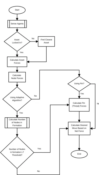
Start

End Sense Agents

Asset Locked In?

Find Closest Asset

Calculate Asset Forces

Calculate Node Forces

Using Adaptive Algorithm?

Number of Nodes in formation LT

Threshold?

Calculate Ftn (Threat) Forces

Using Ftn?

Calculate Number of Nodes in

Formation Calculate Desired

Move Based on Net Force No

No

No Yes

Yes

No

[image:51.595.147.469.85.651.2]

Yes

(52)

0.5 1.0 1.5 2.0 2.5 3.0 Distance 1

2 3 4 Potential

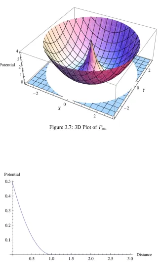
Figure 3.6:Pan, the potential field assets exert on nodes

Pan(dr) =   

αrn(dr−ddrn)2 , dr< ddrn

αan(dr−ddrn)2 , ow

(3.4)

UsingPan, the nodes will be attracted to the desired distance,ddrn, away from the asset,

utilizing an attractive force pulling nodes towards it, and repulsive forces pushing the nodes

away from it.Panitself will not spread the nodes near it into a uniform formation around it,

which would have all the nodes equally spaced while remainingddrnaway from the asset.

For this the intra-nodal potential field,Pnn is introduced.

Pnn(dnn) =   

ηrn(dnn−ddnn)2 , dnn < ddnn

0 , ow

(3.5)

Pnn is a fully repulsive field which will repel other nodes until the desired minimum

node-node distance, ddnn. This field will also seek to mitigate node-node collisions as

the repulsive force will increase as the nodes get closer together. ddnn should be greater

than the desired node-node distance when in formation so the nodes will be forced into

equilibrium, with equal node-node forces on either side. In this manner, if a node leaves

(53)

-2

0

2

X -2

0 2

Y 0

1 2 3 4

[image:53.595.151.474.113.647.2]

Potential

Figure 3.7: 3D Plot ofPan

0.5 1.0 1.5 2.0 2.5 3.0 Distance

0.1 0.2 0.3 0.4 0.5 Potential

[image:53.595.149.468.127.360.2]

(54)

Figure 3.9: Insufficient protection for an asset that allows multiple access points for a threat to compromise protection

The result of these two fields yields the necessary node intelligence for the nodes to

enter formation around the asset in order to protect it from threats, given that the number

of nodes in formation is sufficient to repel the threats(s).

Noting the equations forPanandPnt, the fields that put the nodes into formation around

the asset, and after making assumptions about the formation of the nodes around the asset,

the coefficient forPnt can be made to repel threats in terms of theαat coefficient inPatas

described in Appendix A.

When there are only a few nodes in formation around the asset the formation naturally

suffers from large gaps in protection due to physical distance between nodes in formation

as seen in Figure 3.9.

3.6.2 Potential Threats exert on Nodes

With flaws in formation as seen in Figure 3.9, if the nodes pay no heed to the threats then

there may remain large gaps for the threats to simply “walk in” and compromise the asset.

Upon this observation a field that the threats influence on the nodes, Ptn, was developed

which somewhat unintuitively attracts the nodes to threats. Ptn was engineered such that

the nodes would not be pulled significantly away from the asset, though it would steer the

(55)

0.5 1.0 1.5 2.0 2.5 3.0 Distance 0.2

0.4 0.6 0.8 1.0 Potential

Figure 3.10:Ptn, the potential field threats exert on nodes

fields, Ptn has a repulsive component to ensure collision avoidance. Ptn is designed to

bring the node’s repulsive force against the threats into play against the encroaching threats

when they otherwise would go unutilized.

Ptn(dnn) =   

τrn(dtn−ddtn)2 , dtn < ddtn

τan(dtn−ddtn)2 , ow

(3.6)

This attractive force from the threat on the nodes has some notable advantages and

disadvantages. As stated before, it can shift the nodes from one side of the asset (that does

not currently need protection) to a side that the threat is approaching from as seen in Figure

3.11. It can also draw nodes from an area of the environment that has not sensed any assets

to protect, and pull them towards an asset at which point the node can contribute to asset

protection. In other cases however, it can weaken a formation that is already sufficient to

block threats from reaching the asset by using the node’s Pnn repulsive forces against the

nodes in formation by opening a hole in the protection that allows the threat to slip in a

compromise the asset.

When multiple threats attack a single asset, when the nodes employPtn the nodes

(56)

Figure 3.11:Ptnsuccessfully stopping a threat from compromising the asset from Figure 3.9

[image:56.595.245.376.146.248.2]

(a) (b)

(57)

[image:57.595.236.389.89.194.2]

Figure 3.13: Nodes includingPtnin their calculations are drawn to the stronger threat force on one side of the asset, exposing the asset to being compromised by a single threat.

Figure 3.14: Overhead view of the local minima problem caused by two assets in close proximity

be compromised by smaller threat forces on the exposed side of the asset as seen in Figure

3.13.

Additionally, multiple assets can create a problem of a minima between the two (or

more) assets resulting in poor formation for all assets involved.

3.6.3 Spring Laws

In an effort to compensate for these weaknesses in protection another form of formation

control was explored utilizing spring laws. Spring laws have been used in distributed

flo