Shaping of molecular weight distribution by iterative learning probability density function control strategies

Shaping of molecular weight distribution by iterative

learning probability density function control strategies

1_{Industrial Control Centre, University of Strathclyde, Glasgow, UK} 2

Control Systems Centre, University of Manchester, Manchester, UK

3

Department of Automation, North China Electric Power University, Beijing, People’s Republic of China

The manuscript was received on 27 February 2008 and was accepted after revision for publication on 1 May 2008.

DOI: 10.1243/09596518JSCE584

Abstract: A mathematical model is developed for the molecular weight distribution (MWD) of free-radical styrene polymerization in a simulated semi-batch reactor system. The generation function technique and moment method are employed to establish the MWD model in the form of Schultz–Zimm distribution. Both static and dynamic models are described in detail. In order to achieve the closed-loop MWD shaping by output probability density function (PDF) control, the dynamic MWD model is further developed by a linear B-spline approximation. Based on the general form of the B-spline MWD model, iterative learning PDF control strategies have been investigated in order to improve the MWD control performance. Discussions on the simulation studies show the advantages and limitations of the methodology.

Keywords: molecular weight distribution (MWD), B-spline model, probability density function (PDF), iterative learning control (ILC)

1 INTRODUCTION

It is widely recognized that the molecular weight distribution (MWD) of a polymer is one of the most important variables to be controlled in industrial polymerization processes because it directly affects many of the polymer’s end-use properties such as thermal properties, stress–strain properties, impact resistance, strength, and hardness [1, 2]. There has been much incentive to control MWD accurately during polymerization. The research into the mod-elling and control of MWD in polymerization has constituted an important area in process control for more than a decade, where the aim is to investigate proper control strategies that can effectively control the shape of MWD following the quality require-ments of the end-use polymer.

MWD control and process optimization require on-line MWD information. With the development of hardware and software sensors for on-line

monitor-ing of the polymerization reactions, some polymer properties can be measured continuously or semi-continuously during operations [3]. However, infor-mation on MWD is still largely provided by mathe-matical models during control since the on-line MWD measurement is an unsolved issue in poly-merization processes. Mechanistic MWD models can be developed under the framework of population balance, which include a set of differential equations describing the dynamics of the reaction species such as initiator, monomer, radicals, and polymers of different chain length. These equations are functions of kinetic mechanism and reaction operation con-ditions of the polymerization process [4]. As the polymer chain length of interest is usually a huge number up to maybe millions, direct solution of these hundreds of thousands of differential equa-tions is infeasible in most real situaequa-tions and there-fore various numerical techniques have been devised to address this issue. Computational methods include the adaptive orthogonal collocation algo-rithm [5, 6] and the method of finite molecular weight moments [7]. Some parameterized or statis-tical methods are also developed for MWD descrip-tion, such as Markov chain [8–10], Flory distribution

[11–13], Stockmayer distribution [14], Weibull dis-tribution [15, 16], and Schultz–Zimm distribution [17, 18]. For many practical problems of linear polymerization under steady state or quasi-steady state conditions, the MWD of polymer chains can be described satisfactorily by the Schulz–Flory distribu-tion [4,19,20]. The general way to develop this type of parameterized distribution model consists of three steps. Firstly, set up the differential equation models for reaction species. Secondly, use the generation function technique to establish the leading moments with respect to the distribution. Thirdly, obtain the parameters of the distribution function from the leading moments by optimization. A number of control strategies have been devel-oped to realize MWD control in batch and semi-batch processes (see reviews in references [21] and [22]). These methods can generally be divided into task level control and execution level control [1]. In the task level control (first step), the optimal time profiles of process operations are determined off-line aiming to attain the desired MWD at the end of the control cycle. The time profiles will be used as set point trajectories of manipulated variables, for instance reaction temperature, initiator concentra-tion, feed rate of the monomer or chain transfer agent, etc. In order to track the optimal trajectory during operations, regulatory control is implemen-ted in the execution level (second step), in which on-line techniques, such as state estimation with extended Kalman filter, are developed to update the MWD information or the manipulated control profiles [1, 21, 23, 24]. Controllers from propor-tional-integral-derivative (PID) to model-based non-linear control such as multivariable predictive con-trol have been attempted in the execution level. MWD control following these two steps can be found in many examples [1,2,21,24–32].

The control efforts in the above discussions should be regarded as open-loop control in terms of the MWD property because the optimal profiles relating to the desired MWD are determined in an off-line manner. To realize closed-loop control of dynamic MWD, the idea of output probability density function (PDF) control allows a unique solution. Here the controller is designed to make the output PDF follow a desired PDF [33]. The development of output PDF control was inspired by requirements from real industries, of which the system output relates to space distribution. In addition to MWD systems, examples also include particle size distribution (PSD) control in polymerization processes, [34–36] PSD control in crystallization and powder industries [37–40], fibre

length distribution control in paper industries [41], flame temperature distribution control in combustion processes [42], etc. Unlike the mean and variance control in Gaussian processes, the output PDF is a function not only of time but also of a space variable. The dynamics of the output PDF can thus be generally described by a partial differential equation (PDE) in terms of both the time and space variables, which defines the PDF shape at each time instant. However, direct use of PDE models is difficult in practice in that either such a model is difficult to establish due to the complicated nature of processes or the obtained control algorithms are too complicated to be applied in real-time situations. The output PDF control strategies were proposed to solve this type of problem [33,43,44], in which the main technique is the use of a set of fixed basis functions together with a group of time-varying weights to approximate the output PDF at each time instant.

Using function approximations in PDF modelling, a large number of basis functions are required when the PDF dynamics is complicated. Since the PDF of a process output can vary widely over operations, it may be unrealistic to capture the output behaviour with fixed basis functions. As a result, it would be ideal to be able to update the basis functions during the control process. This is especially suitable for systems that have a nature of repetitive closed-loop operations such as the batch-to-batch processes in chemical engineer-ing. These batches are iterative by nature and in practice it is expected that the closed-loop perfor-mance becomes improved from batch to batch. In this context, the iterative learning control (ILC) could be very well applied [45,46]. The important aspect in ILC is to update the control input in thekth batch from the control in the (k–1)th batch plus a correction term that is related to the closed-loop performance of the kth batch. This strategy has the advantage of improving the closed-loop system performance along with the progress of the operation [47,48].

In this work, two iterative learning PDF control methods have been attempted in the closed-loop MWD control of a simulated semi-batch polymer-ization process. The paper is structured as follows. In section 2, development of the static and dynamic MWD models is presented. The first-principle model is then approximated by a linear B-spline model in an iterative form in section 3. In the fourth section, the methodology of iterative learn-ing PDF control is outlined. The simulated case study of MWD shaping by iterative learning PDF control is presented in section 5. Conclusions are given in the final section.

2 MWD MODEL DEVELOPMENT

2.1 The styrene polymerization process

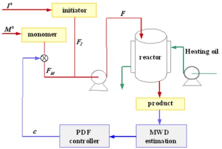
The process of interest is a simulated styrene polymerization system in a semi-batch reactor. Styrene is the monomer for polymerization and azobisisobutyronitrile is the initiator. These two flows are injected into the reactor with a ratio between them that can be adjusted. The reaction temperature is assumed to be kept constant during the reaction process. The total flowrate to the system, F, is composed of the monomer flow, FM, and the initiator flow, FI, i.e. F5FM+FI. The monomer input ratio is defined as

c~ FM

FIzFM

ð1Þ

The output MWD will be changed when the ratiocis changed. In this presented work, the monomer input ratio c is selected as the control input. When the flowrate of the initiator is fixed, the change in c

corresponds to the change in the monomer flowrate. It is a common practice to use the flowrate of the monomer as a manipulated variable in batch or semi-batch MWD control systems [28]. The poly-merization system is shown in Fig. 1.

The following free radical polymerization mechan-isms are considered in the modelling:

(a) Initiation

IK?d 2R1 R1z_MK_?i _R1

(b) Chain propagation

RjzM? Kp

Rjz1

(c) Chain transfer to monomer

RjzM? Ktrm

PjzR1

(d) Termination by combination

RjzRi ? Kt

Pjzi

whereI is the initiator,Mis the monomer,R*is the primary radical, Rj is the live polymer radical with chain length j, Pj is the dead polymer with chain lengthj, andKd,Ki,Kp,Ktrm, andKtare reaction rate constants. The following mass balance equations are derived to describe the concentrations of the reac-tion species

dI

dt~ I0_{I

h {KdI ð2Þ

dM

dt ~

M0_{M

h {2KiI{ KpzKtrm

MR ð3Þ

dR1 dt ~{

R1

h z2KiI{KpMR1

z_{KtrmM Rð} {_R1Þ{_{KtR1R ð4Þ}

dRj

dt ~{ Rj

h {KpM Rj{Rj{1

_{

KtrmMRj

{_{KtRjR ðj}o_{2Þ ð5Þ}

Fig. 1 Simulated semi-batch MWD control system

DA

DA

dP2

dt ~KtrmR2MzKtR

2

1{

P2

h ð6Þ

dPj

dt ~KtrmRjMz Kt

2 Xj{1

l~1

RlRj{l{

Pj

h ðjo3Þ ð7Þ

whereh5V/F(Vis the volume of the reactor) is the average residential time of the reactants in the reactor and

R~X ?

j~1

Rj ð8Þ

is the total concentration of the radicals. To use the generation function technique, denoting

P~X ?

j~2

Pj ð9Þ

as the total concentration of the dead polymers, the following formulation can be obtained from equa-tions (4) to (9) to give

dR

dt ~{ R

hz2KiI{KtR

2 _ð10Þ

dP

dt~{ P

hzKtrmM Rð {R1Þz

Kt 2R

2 _ð11Þ

R1in equation (11) can be ignored compared withR

because of its low concentration, i.e.

dP

dt~{ P

hzKtrmMRz

Kt 2 R

2 _ð12Þ

2.2 Static MWD model

The static solutions to the concentrations of the reaction species can be derived from their dynamic equations. Denote

a~₁zKtrm

Kp

z KtR

KpM

z 1

KpMh

ð13Þ

By taking equations (2), (3), (10), and (12) to be zero, then

I~ I 0

1z_Kdh ð14Þ

R~ {₁

hzqffiffiffiffiffiffiffiffiffiffiffiffiffiffiffiffiffiffiffiffiffiffiffiffiffiffiffiffi_1h2z_8KtKiI

2Kt

ð15Þ

M~ M

0

1z_Kpz_KtrmRh ð16Þ

P~_{h KtrmMR}zKt 2R

2

ð17Þ

Similarly, from equations (4), (5), (6), and (7), the static concentrations of radicals and polymers are

R1~2KiI

z_KtrmMR

KpMa

ð18Þ

Rj~a{1Rj{1~a{ðj{1ÞR1 ðjo2Þ ð19Þ

P2~h KtrmMR2zKtR21

ð20Þ

Pj~h KtrmMRjz

Kt 2

Xj{1

l~1

RlRj{l

!

jo3

ð Þ ð21Þ

Substituting equation (19) into (20) and (21) and divided byP, the normalized MWD at static state can be obtained to be

Pj~

h

P a {1_K

trmMR1zKtR21

j~₂

h

P a {ðj{1Þ_K

trmMR1

zj{1 2 a

{ðj{2Þ_K tR21

jo3 8

> > > > > > < > > > > > > :

ð22Þ

It can be seen from equation (22) that

X?

j~2

Pj~1 ð23Þ

Therefore, the static MWD can be taken as a discrete PDF of the chain lengthj.

2.3 Dynamic MWD model

For the dynamic MWD model, the distribution ofPj

function of time. At each time instance, the moment method is used for the MWD description.

The moments of the number chain-length dis-tributions of radicals and polymers are defined as

Uk~

X

z?

j~1

jk_R

j, k~0,1,2, . . . ð24Þ

Zk~

X

z?

j~2

jk_P

j, k~0,1,2, . . . ð25Þ

It can be seen from equations (8) and (9) thatU05R

and Z05P. For the radicals, the differential equa-tions of the leading moments are derived using the generation function technique as follows

dU0 dt ~{

U0

h z2KiI{KtU 2

0 ð26Þ

dU1 dt ~{

U1

h z2KiIzKpU0M{KtU0U1

z_{KtrmM Uð 0}{_{U1Þ ð27Þ}

dU2 dt ~{

U2

h z2KiIzKpMð2U1zU0Þ

{_KtU0U2z_{KtrmM Uð 0}{_{U2Þ ð28Þ}

Similarly, the three leading moments of the poly-mers are derived to be

dZ0 dt ~{

Z0

h zKtrmMU0z

Kt 2 U

2

0 ð29Þ

dZ1 dt ~{

Z1

h zKtrmMU1zKtU0U1 ð30Þ

dZ2 dt ~{

Z2

h zKtrmMU2zKtU0U2zKtU 2

1 ð31Þ

The mean and variance of the MWD are related to the moments by

m~ Pz_?

j~2jPj

Pz?

j~2Pj

~Z1

Z0

ð32Þ

s2~ Pz?

j~2ðj{mÞ

2_P

j

Pz?

j~2Pj

~Z2

Z0 {Z 2 1 Z2 0

ð33Þ

Theoretically, an exact formulation of MWD requires countless number of moments, which is infeasible in practical computation. An alternative method is to choose a distribution function to approximate the real MWD. For the polymer discussed in this work, the well-known Schultz–Zimm distribution is considered to be suitable for the MWD description. With this function, a simple analytical expression for the scat-tering from the distribution is available. The normal-ized Schultz–Zimm distribution is defined as [53]

f nð Þ~h

h_nh{1_{exp {hn=M}

n

ð Þ

Mh nCð Þh

no1

ð Þ ð34Þ

where n is the chain length, h is a parameter indicating the distribution breadth, Mn is the number average chain length which is defined as

Mn5Z1/Z0, andCis the gamma function defined as Cð Þh~Ð?

0 n

h{1_e{n_{dn. When h51, the Schultz–}

Zimm distribution reduces to the exponential Flory distribution, which is another commonly used distribution for MWD. The mean and variance of the Schultz–Zimm distribution are

m~ ð?

0

nf nð Þdn~ ð?

0

hh_nh_{exp {hn=M} n)

ð Þ

Mh nCð Þh

dn

~_{Mn ð35Þ}

s2~ ð?

0

n{_m

ð Þ2f nð Þdn~hz1

h M

2

n{m2 ð36Þ

By comparing equations (32) and (33) with (35) and (36), the two parameters of the Schultz–Zimm distribution are found to be

h~ Z 2 1

Z0Z2{Z12

ð37Þ

Mn~Z1=Z0 ð38Þ

The first-principle model describes the entire MWD by a Schultz–Zimm distribution. From the model development process, it can be seen that the parameters of the distribution function are linked to the dynamic process via moments of polymers and concentrations of reaction species.

The calculation of the dynamic MWD can be summarized in the following three steps:

1. ObtainZ0,Z1,Z2from equations (2), (3), and (26)

to (31).

3. Formulate the MWD by equation (34).

3 B-SPLINE APPROXIMATION FOR ITERATIVE

LEARNING CONTROL

Though the first-principle model has the ability of predicting MWD dynamically, it will not be used directly in MWD control. Instead, a B-spline approx-imation model is established from the data produced by the first-principle model. The reason for doing so is that rather than taking the MWD control as a specific problem, it is more general to treat it as a problem with the output being a function of time and space variables. Also, when using a general B-spline model, even if the first-principle model is not available, the PDF control strategy can still be applied with the measurement of MWD if online techniques permit. Here the well-established B-spline PDF model is redeveloped to suit the purpose of iterative learning PDF control in the MWD system.

3.1 Output PDF model with fixed B-spline functions

Consider a continuous PDFci(y) defined on the [a,b]

interval. The linear B-spline neural network can be used to give an approximation of ci(y) [33]

c_ið Þy ~X

n l~1

vlð Þui Blð Þy ze0 ð39Þ

where the subscriptiindicates the ith sample time. Throughout the paper, ci(y) is assumed to be

measurable, ui is the control input at time i(i51, 2, …, m), m is the total sample number along the time axis,Bl(y)(l51, …,n) are the pre-specified basis functions defined on the interval ofy[[a,b],nis the total number of the basis functions used for the approximation to ci(y), vl(ui)(l51, …, n) are

the expansion weights, and e0 represents the approximation error which satisfies |e|,d1 (d1 is a

known small positive number). To simplify the expression, e0 is neglected in the following. Due to the fact that the integration of a PDF over its definition domain should be 1, there are only n– 1 independent weights out of the original n weights [44]. Using this B-spline approximation and con-sidering linear dynamics in the weights vector, the following discrete output PDF model is formulated

Vi~AAVi{1zBBui{1 ð40Þ

c_ið Þy ~_{Cð Þy Vi}z_{L yð Þ ð41Þ}

whereVi5[v1(ui),v2(ui), …,vn–1(ui)]Tis the weights

vector of the B-spline model at timei. A¯ andB¯ are the system parameter matrices of proper dimen-sions. C(y) and L(y) are related to the B-spline functions by

Q_l~ ðb

a

Blð Þy dy, l~1, . . .,n

L yð Þ~_{Bnð Þ=y Qn}

crð Þy ~Brð Þy {L yð ÞQr, r~1, . . .,n{1

Cð Þy ~½_{c1ð Þy ,c2ð Þy ,} . . .,cn{1ð Þy

3.2 B-spline model in iterative form

In order to formulate the ILC law for batch-to-batch PDF control, the system model is written as

Vk,i~AAkVk,i{1zBBkuk,i{1 ð42Þ

c_k,ið Þy ~_{Ckð Þy Vk,i}z_{Lkð Þy ð43Þ}

where the added subscriptkindicates thekth batch andck,i(y),Vk,i, anduk,iare the output PDF, weights

vector, and control input respectively at the ith sample time in thekth batch. For thekth batch,Ck(y)

andLk(y) are formulated to be

Q_k,l~ ðb

a

Bk,lð Þy dy, l~1, . . .,n ð44Þ

Lkð Þy ~Bk,nð Þy Qk,n ð45Þ

ck,rð Þy ~Bk,rð Þy {Lkð Þy Qk,r, r~1, . . .,n{1 ð46Þ

Ckð Þy ~ ck,1ð Þy , ck,2ð Þy , . . ., ck,n{1ð Þy

ð47Þ

The input–output expansion of (42) and (43) is as follows

fk,ið Þy ~ck,ið Þy {Lkð Þy

~X

n{1

p~1

ak,pfk,i{pð Þy z

X

n{2

q~0

with Dk,q5[dk,q,1, dk,q,2, …, dk,q,n–1]T, which are

directly related to matrices A¯_kandB¯_k. Denoting

hk~ak,1, . . .,ak,n{1,dk,0,1, . . .,dk,0,n{1, . . .,

dk,n{2,1, . . .,dk,n{2,n{1

w_k,ið Þy ~_{fk{1,i{1ð Þy , . . .,fk{1,i{nz1ð Þy ,}

ck,1ð Þy uk{1,i{1, . . .,ck,n{1ð Þy uk{1,i{1, . . .,

ck,1ð Þy uk{1,i{nz1, . . .,ck,n{1ð Þy uk{1,i{nz1

equation (48) can be further expressed by

fk,ið Þy ~wk,ið Þy hTk ð49Þ

This is similar to the standard form of a linear system whose parameters in hk can be estimated by

least-squares identification methods.

Within each batch, such a PDF model has been fully explained in some previous work [33, 43, 44]. However, different from the model with fixed B-splines, the iterative model features different basis functions for each batch, which means that the B-spline functions for the PDF approximation can be updated iteratively from batch to batch in order to improve the modelling accuracy. This is important for real systems modelling where the process is normally in a time-varying and uncertain environment. For the linear weights model used in this work, the iterative update of the B-spline model also helps to address the system’s non-linear nature to some extent.

3.3 Parameter re-estimation for the updated B-spline functions

In the iterative learning PDF control cycle, the B-spline basis functions are updated from batch to batch (this will be further explained in the next section). In each batch, when the updated basis functions are taken for PDF approximation, the model parameters in (49) need to be re-estimated.

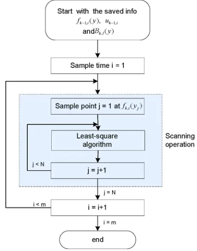
At each sample timeiin thekth batch, fk,i(y) is a continuous function of y defined on [a,b]. Assume that fk,i(y) can be represented by N sample points;

then for each sample point jthere is

fk,i yj ~wk,i yj hTk, j~1, . . .,N ð50Þ

As a result, with respect to the new index j, the following least-squares algorithm can be used to estimatehkbased on the measured output PDFs, the

control inputs in the (k–1)th batch, and the adjusted

B-spline functions

^

h

hkðjz1Þ~^hhkð Þj z

Pð Þj wT_k,i yj ekð Þj

1z_{wk,i yj Pð Þj w}T

k,i yj

ð51Þ

ekð Þj ~fk,i yj {wk,i yj ^hhkð Þj ð52Þ

P_ðjz_1Þ~ _I{ Pð Þj w T

k,i yj wk,i yj

1z_{wk,i yj Pð Þj w}T

k,i yj

!

Pð Þj ð53Þ

whereP¯(1)5103–6I(n–1)6n. The recursive loops of the

identification algorithm is shown in Fig. 2, in which the inner loop operation is called ‘scanning’ because the variable yj goes through the whole definition interval of [a,b] by j51, …,N.

4 ITERATIVE LEARNING PDF CONTROL

4.1 Iterative learning algorithm I

4.1.1 Iterative update of the B-spline model

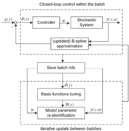
The sketch of the iterative learning PDF control is shown in Fig. 3, in whichuis the control input,c(y,u) is the output PDF,g(y) is the target PDF,d(y) measures the distance between the output PDF and the target PDF. This algorithm consists of three steps:

1. Update the B-spline basis functions from the PDF control error in the previous batch.

2. Re-estimate the parameters of the B-spline model with the updated basis functions.

3. Design the PDF controller using the updated B-spline model and apply it to the current batch.

In this paper, the following polynomial B-spline is used to approximate the output PDF

Bk,lð Þy ~

{4hk,l

w2

k,l

y{_yl0{wk,l 2

2

z_{hk,l, y[yl0,yl0}z_wk,l

0, otherwise

8 > < > :

ð54Þ

forl51, …,n. Herehk,landwk,lstand for the height and width of each B-spline basis function with

Bk,l(y)>0, hk,l>0 and wk,l>0, and [yl0, yl0+wk,l] is thelth subinterval within [a,b]. As the width of the basis functions are tuned between batches, the subinterval [yl0,yl0+wk,l] will shift within [a,b] batch by batch. It can be seen thathk,landwk,ldetermine the shape of the basis functions.

Substituting (54) into equations (44), (45), and (46) gives

Q_k,l~ ðb

a

Bk,lð Þy dy

~ ðbk,l

ak,l

{4hk,l

w2

k,l

y{_yl0{wk,l 2

2

z_hk,l

" #

dy

forl~_1, . . .,n

ð55Þ

Lkð Þy ~

{ _4hk,n._w2

k,n

y{_yn0{_wk,n2

2

z_hk,n Q_k,n ð56Þ

ck,rð Þy ~{

4hk,r

w2

k,r

y{_yr0{wk,r 2

2

z_hk,r

{_{Lkð Þy Qk}

,r, r~1, . . .,n{1 ð57Þ

whereak,l andbk,l are the lower and upper bounds for the lth B-spline basis function in the kth batch and ak,l5yl0, bk,l5min(yl0+wk,l, b). When y[[ak,l,

bk,l], the inequalityBk,l(y)>0 is assured.

The iterative update of the basis functions are based on all the PDF tracking errors collected at each sample time from the previous batch. Denote the 2-norm PDF tracking error at sample timeiin the (k– 1)th batch as

dk{1,i~

ðb

a

ck{1,ið Þy {g yð Þ

2

dy ð58Þ

whereg(y) is the target PDF. It can be seen thatdk–1,i

>0. The error vector that groups all themsampling errors in the (k–1)th batch can be represented by

Ek{1~ dk{1,1,dk{1,2, . . .,dk{1,m

T

ð59Þ

For the B-spline basis functions defined in (54), the following P-type iterative learning law is adopted to adjust the parametershk,landwk,lso as to tune the shape of the functions

Hk~Hk{1zQHEk{1 ð60Þ

Wk~Wk{1zQWEk{1 ð61Þ

whereHk5[hk,1, …,hk,n]TandWk5[wk,1, …,wk,n]T

are the vectors composed of the height and the width of each B-spline basis function in the kth (k>2) batch. QH and QW are the learning rate

matrices to be determined.

Algorithm (58) to (61) shows that at each tuning interval, the basis functions are updated using the PDF tracking errors collected from the previous batch. In addition, it can be seen from equations (58) and (59) that all the variables inEk–1are always non-negative. This shows that the learning ratesQHand

QWcan be either positive or negative, which allows

functions to either increase or decrease after the tuning via equations (60) and (61). Once the basis functions are updated, the parameters of the B-spline model will be re-estimated, as presented in section 3.3.

The PDF controller is designed with the updated model by optimizing the following quadratic perfor-mance function

Jk,i~

ðb

a

c_k,ið Þy {_{g yð Þ}

2

dyz_uk,iRuT

k,i ð62Þ

where R.0 is a pre-specified weighting factor. Taking qJk,i/quk,i50, the control input is developed to be

uk,i~

Ðb

aCkð Þy Dk,0gg~k,ið Þy dy

Ðb

a Ckð Þy Dk,0)

2

dyz_R ð63Þ

where

~ g

gk,ið Þy ~{

X

n{1

p~2

ak,pfk,i{pz1ð Þy zCkð Þy Dk,p{1uk,i{pz1

{_{Lkð Þy} z_{g yð Þ}{_{ak,1fk,ið Þy}

is a known term at the ith time instance in thekth batch.

4.1.2 Convergence analysis

In order to guarantee the convergence of the proposed iterative learning algorithn for PDF control, appro-priate learning rates in equations (60) and (61) should be chosen to tune the B-spline basis functions so that the controller can progressively improve the tracking performance batch by batch, which eventually leads to a satisfactory output PDF tracking with respect to the desired PDF. For this purpose, the following two aspects are considered to formulate some guidelines to the selection of the learning rates:

1. The weight and height of all the basis functions should always be kept non-negative, i.e.hk,l>0 and wk,l>0,l51, …,n. This constraint comes from the

definition of the B-spline functions in (54).

2. For a gradually improved iterative learning algo-rithm, the sum of the tracking errors should be reduced batch by batch, i.e.

0v

Pm i~1dkz1,i

Pm i~1dk,i

¡1 ð64Þ

Denoting

Dk~

Xm

i~1

dk,i ð65Þ

the inequality (64) can be expressed as

0vDkz1

Dk

¡1 ð66Þ

The above sufficient conditions guarantee that the iterative leaning rules (60) and (61) are convergent and that the PDF tracking error decreases batch by batch. Assuming that the learning incrementsQHEk

and QWEk are small, the following first-order

approximation can be made

Dkz1&Dkz

LD

LH H~H_k,W~W_k

T

:_Q

HEk

z LD

LW H~Hk,W~Wk

T

:_Q

WEk ð67Þ

This leads to

Dkz1 Dk

&1z LD=LH H~Hk,W~Wk

T_:

QHEk

Dk

z LD=LW H~Hk,W~Wk

T_:

QWEk

Dk

ð68Þ

Taking (68) into (66) yields

0v1z

LD=LH H~Hk,W~Wk

T_:

QHEk

Dk

z LD=LW H~Hk,W~Wk

T_:

QWEk

Dk

¡1 ð69Þ

It is known thatDk.0 from (65); therefore

{_Dkv LD

LH H~Hk,W~Wk

T

:_Q

HEk

z LD

LW H~Hk,W~Wk

T

:_Q

WEk¡0 ð70Þ

When the selection of the learning ratesQHandQW

satisfy (70), a convergent ILC law will be guaranteed.

4.2 Iterative learning algorithm II

batch to batch, which increases modelling accuracy progressively but also increases the computational load. To overcome this problem, an alternative way is to update the control sequence in the current batch from the PDF control errors in the previous batch without changing the model.

Again, taking the performance function in equa-tion (62), the tracking error vector for the kth iteration is defined as in equation (59). Following the iterative learning rule, the control input at theith time in the current batch should be updated based on the control input and tracking errors in the previous batch, i.e.

ukz1,i~uk,izykz1ði,iÞEkð Þi ð71Þ

where yk+1 is the diagonal learning rate matrix for

the (k+1)th batch. The learning rates should be chosen to guarantee the asymptotical convergence of the algorithm, i.e.

Xm

i~1 dk,i¡

Xm

i~1

dk{1,i ð72Þ

Denoting the compensation term in (71) as

Duk,i~ykz1ð Þi,i Ekð Þi ð73Þ

condition (72) can be satisfied equivalently when

Xm i~1

Ldk,i

LDuk{1,i{1

v0 ð74Þ

Taking the PDF model (42) and (43) into dk,i, the

following equation can be derived

Ldk,i

LDuk{1,i{1 ~₂

ðb

a

F

Fkð Þy Duk{1,i{1FFkð Þy dy

z₂ ðb

a

E

Ekð Þy Vk,i{1zFFkð Þy uk{1,i{1

z_{ggkð Þy} |_{FFkð Þy dy ðio2Þ ð75Þ}

where E¯k(y)5Ck(y)A¯k, F¯k(y)5Ck(y)B¯k, g¯k(y)5Lk(y)– g(y). Therefore, (74) turns out to be

Xm i~1

ðb

a

F

Fkð Þy Duk{1,i{1FFkð Þy dy

v{

Xm

i~1 ðb

a

E

Ekð Þy Vk,i{1zFFkð Þy uk{1,i{1zggkð Þy

|_{FFkð Þy dy ðio1Þ ð76Þ}

Taking (73) into (76) gives

Xm i~1

ðb

a

F

Fkð Þy ykði{1,i{1ÞEEk{1ði{1ÞFFkð Þy dy

v{

Xm

i~1 ðb

a

E

Ekð Þy Vk,i{1zFFkð Þy uk{1,i{1zggkð Þy

|_{FFkð Þy dy ð77Þ}

The learning matrixykshould be designed to satisfy

the condition in (77) for the asymptotical conver-gence of the closed-loop system.

5 CASE STUDY OF MWD CONTROL

The case for study is the semi-batch polystyrene process presented in section 2.1. To start with, the first-principle MWD model is developed to produce the dynamic MWD data and then the MWD data are used to set up the B-spline approximation model. The PDF control strategies are developed and implemented based on the B-spline model. The simulation conditions for the MWD system are given in Table 1. Comparisons are made between the two iterative learning PDF control strategies and the standard PDF control. In all the simulations, the initial MWD corresponds to the MWD under the monomer input ratio ofc50.4, and the target MWD is the one corresponding to c50.6. A physical constraint of 0.4(c(0.8 is considered for the monomer input ratio.

5.1 MWD control by standard PDF control

For a standard PDF control based on the fixed B-spline model, the control law is

ui~

Ðb

aCð Þy D0gg~ið Þy dy

Ðb

aðCð Þy D0Þ

2

dyz_R ð78Þ

In order to obtain the necessary modelling accuracy, 10 third-order B-spline functions are selected for the MWD approximation. The standard PDF control was performed withR5661026_{. The selection of R is a}

moved towards the target MWD, but the steady state tracking error remains when the control action is convergent.

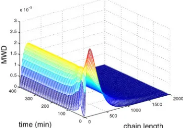
5.2 MWD control by iterative learning algorithm I In this ILC-PDF control simulation, five third-order B-spline functions are used in the MWD approxima-tion. The interval in each batch is set to be 600 minutes. The simulation results are shown in Figs 7 to 10. It is observed from the simulation process that this control algorithm is computationally extensive

since the B-splines need to be updated from batch to batch. Also, in order to satisfy the convergent condition in (70), the learning factors have to be adjusted several times in each batch, which further increases the computational effort. The results show that the distance between the output MWD and the target MWD can be reduced from batch to batch by the ILC strategy (see Fig. 8) with the reduced number of B-splines. However, the tuning ability is

Table 1 MWD system parameters

Kd 9.4861016exp(230798.5/rT Ki 0.6Kd

Kp 6.3066108exp(27067.8/rT)

Ktrm 1.3866108_{exp(212671.1/rT)} Kt 3.76561010exp(21680/rT)

V 3.927

F 0.0286

T 353

I0 _0.0106

M0 4.81

r 1.987

c [0.4, 0.8]

Fig. 4 Control input with standard PDF control

Fig. 5 MWD evolutions with standard PDF control

Fig. 6 Initial, target and final MWDs with standard PDF control

Fig. 7 Control input with the ILC-PDF algorithm I

saturated after several batches. This leaves the MWD tracking error at the end of the iterative learning cycle.

5.3 MWD control by iterative learning algorithm II

In this simulation, 10 third-order B-spline functions are selected for the MWD approximation. The interval length in each batch is set to be 400 minutes. The standard PDF control was implemented in the first batch with R5661026 _{and then the iterative}

learning algorithm II was applied. Results are displayed in Figs 11 to 14. Although the steady state tracking errors remained in the first batch, the algorithm achieves a perfect tracking after another several batches. The cumulative error is decreasing from batch to batch.

Comparing the ILC-PDF controllers with the standard PDF controller, the ILC algorithm I uses a lower number of B-splines in modelling and it can achieve the decreasing tracking errors progressively.

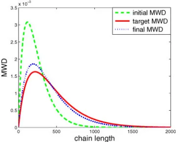
However, this algorithm is computationally expen-sive and, at least to this example, it could not eliminate the MWD tracking errors at the end of the control cycle. In the second algorithm, the model is updated in each batch and then the standard PDF control strategy is applied based on the updated model. The convergence condition is given to guarantee the decrease of MWD tracking errors from batch to batch. Nevertheless, the improvement of Fig. 9 Initial, target, and final MWDs with the

ILC-PDF algorithm I

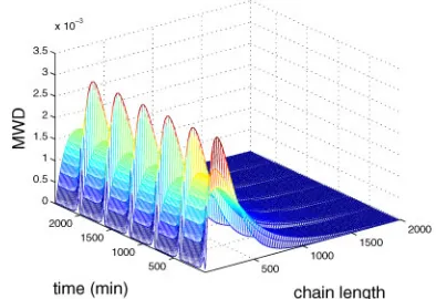
Fig. 10 Batch-to-batch MWD evolutions with the ILC-PDF algorithm I

Fig. 11 Control input with the ILC-PDF algorithm II

Fig. 12 Cumulative errors in each batch with the ILC-PDF algorithm II

the modelling accuracy cannot be guaranteed by the current tuning principle and therefore the tracking errors may still remain after the tuning is conver-gent. By employing the second iterative learning algorithm, the B-spline model does not need to be updated during the process and the control input in the current batch is adjusted according to the MWD tracking errors in the previous batch. This is a simple solution compared with the first ILC-PDF control algorithm, but it can achieve perfect MWD tracking after several batches. The function of batch-to-batch tuning based on the previous tracking errors is equivalent to the integral efforts in feedback control and is therefore capable of eliminating tracking errors. This means that the fundamental principle of iterative learning control enables performance improvement in output PDF control.

6 CONCLUSIONS

The challenging problem of feedback MWD control has been studied in this work. It is different from most of the current control strategies on MWD shaping because the complete MWD is controlled as a closed-loop variable under the framework of output PDF control. Iterative learning strategies have been attempted to improve the control quality. It can be seen from the case study that even for a simulated MWD system, the model is highly com-plex and it is difficult to achieve the perfect PDF tracking when using linear B-spline models and employing the standard output PDF control strategy. Introducing the idea of iterative learning control into output PDF control does improve the control performance in that it can reduce the PDF control errors from batch to batch. The present methods are developed based on B-spline models which becomes computationally challenging when the system is

complicated. It is worth further efforts in exploring different modelling methodology that would be more convenient for online iterative learning con-trol. To provide more benefit from the ILC’s advantages, investigations on developing efficient learning algorithms in both modelling and control are required in future work.

ACKNOWLEDGEMENT

The authors would like to thank Professor Liulin Cao from Beijing University of Chemical Technology for her great help in MWD model development. This work was supported by Chinese NSFC 307705660 and 60534010 and the 111 Project (B08015) with the Northeastern University of China which the second author is affiliated to. These are gratefully acknowl-edged.

REFERENCES

1 Crowley, T. J.andChoi, K. Y.Experimental studies on optimal molecular weight distribution control in a batch-free radical polymerization process.

Chem. Engng Sci., 1998,53(15), 2769–2790. 2 Takamatsu, T., Shioya, S., and Okada, Y.

Mole-cular weight distribution control in a batch poly-merization reactor. Ind. Engng Chem. Res., 1988, 27(1), 93–99.

3 Kammona, O., Chatzi, E. G., andKiparissides, C. Recent developments in hardware sensors for the on-line monitoring of polymerization reactions. J. Macromolec. Sci., Rev. Macromolec. Chem. Phys., 1999,C39(1), 57C134.

4 Pinto, J. C. A matrix representation of polymer chain size distributions, 1. Linear polymerization mechanisms at steady-state conditions. Macromo-lec. Theory Simulation, 2001,10(2), 79–99.

5 Nele, M., Sayer, C.,andPinto, J. C.Computation of molecular weight distributions by polynomial approximation with complete adaptation proce-dures.Macromolec. Theory Simulations, 1999,8(3), 199–213.

6 Sayer, C., Aranjo, P. H. H., Arzamendi, G., Asua, J. M., Elma, E. L.,andPinto, J. C.Modeling mole-cular weight distribution in emulsion polymeriza-tion reacpolymeriza-tions with transfer to polymer. J. Polym. Sci. A: Polym. Chem., 2001,39(20), 3513–3528. 7 Crowley, T. J. and Choi, K. Y. Calculation of

molecular weight distribution from molecular weight moments in free radical polymerisation.

Ind. Engng Chem. Res., 1997,36(5), 1419–1423. 8 Christov, L. and Georgiev, G. An algorithm for

determination of the copolymer molecular weight distribution by Markov chain simulation. Macro-molec. Theory Simulations, 1995,4(1), 177–193. Fig. 14 Batch-to-batch MWD evolutions with the

9 Storti, G., Polotti, G., Cociani, M.,andMorbidelli, M. Molecular weight distribution in emulsion polymerization. I. the homopolymer case.J. Polym. Sci. A: Polym. Chem., 1992,30, 731–750.

10 Storti, G., Polotti, G., Cociani, M.,andMorbidelli, M. Molecular weight distribution in emulsion polymerization. II. The copolymer case. J. Polym. Sci. A: Polym. Chem., 1992,30, 751–777.

11 Flory, P. J. Principles of polymer chemistry, 1953 (Cornell University Press, Ithaca, New York). 12 Soares, J. B. P.andHamielec, A. E.Deconvolution

of chain-length distributions of linear polymers made by multiple-site-type catalysts. Polymer, 1995,36(11), 2257–2263.

13 Soares, J. B. P., Kim, J. D., and Rempel, G. L. Analysis and control of the molecular weight and chemical composition distributions of polyolefins made with metallocene and Ziegler–Natta cata-lysts. Ind. Engng Chem. Res., 1997, 36(4), 1144–1150.

14 Stockmayer, W. H. Distribution of chain lengths and compositions in copolymers. J. Chem. Phys., 1945,13, 199.

15 Cao, L. and Yue, H. Mathematical models of

microscopic quality for polybutadiene production.

J. Beijing Inst. Chem. Technol., 1994,21(2), 65–69. 16 Yue, H.andCao, L.Reaction extent modeling of a

butadiene polymetization process. In Proceedings of the IFAC International Symposium onAdvanced control of chemical processes, Pisa, Italy, 14–16 June 2000, pp. 1043–1048.

17 Cao, L.andLu, N.Modelling of a continuous PET process.J. System Simulation, 2001,13(4), 536–538. 18 Yue, H., Wang, H.,andCao, L.Control oriented B-spline modelling of a dynamic MWD-system. In Proceedings of the IFAC International, Symposium on Advanced control of Chemical Processes, Gra-mado, Brazil, 2–5 April 2006, pp. 719–724.

19 Nele, M.andPinto, J. C.Molecular-weight multi-modality of multiple Flory distributions. Macro-molec. Theory Simulation, 2002,11(3), 293–307. 20 Salazar, A., Gugliotta, L. M., Vega, J. R.,andMeira,

G. R. Molecular weight control in a starved emulsion polymerization of styrene. Ind. Engng Chem. Res., 1998,37(9), 3582–3591.

21 Kiparissides, C.Challenges in particulate polymer-ization reactor modeling and optimpolymer-ization: a population balance perspective.J. Process Control, 2006,16(3), 205–224.

22 Yue, H., Wang, H.,andZhang, J. F.Modelling and control of molecular weight distribution in poly-merization processes. Control Instrum. Chem. Industry, 2004,31(6), 1–7.

23 Ellis, M. F., Taylor, T. W.,andJensen, K. F.On-line molecular weight distribution estimation and con-trol in batch polymerization.Am. Inst. Chem. Engrs J., 1994,40(3), 445–462.

24 Kiparissides, C., Seferlis, P., Mourikas, G., and Morris, A. J. Online optimizing control of mole-cular weight properties in batch free-radical

poly-merization reactors. Ind. Engng Chem. Res., 2002, 41(24), 6120–6131.

25 Alhamad, B., Romagnoli, J. A., andGomes, V. G. Advanced modelling and optimal operating strat-egy in emulsion copolymerization: application to styrene/MMA system. Chem. Engng Sci., 2005, 60(10), 2795–2813.

26 Alhamad, B., Romagnoli, J. A., andGomes, V. G. On-line multi-variable predictive control of molar mass and particle size distributions in free-radical emulsion copolymerization. Chem. Engng Sci., 2005,60(23), 6596–6606.

27 Chang, J.-H. and Liao, P.-H. Molecular weight control of a batch polymerisation reactor: experi-mental study. Ind. Engng Chem. Res., 1999, 38(1), 144–153.

28 Clarke-Pringle, T. L. and MacGregor, J. F. Opti-mization of molecular-weight distribution using batch-to-batch adjustments. Ind. Engng Chem. Res., 1998,37(9), 3660–3669.

29 Crowley, T. J. and Choi, K. Y. Discrete optimal control of molecular weight distribution in a batch free radical polymerization process. Ind. Engng Chem. Res., 1997,36(9), 3676–3684.

30 Echevarria, A., Leiza, J. R., de la Cal, J. C., and Asua, J. M.Molecular weight distribution control in emulsion polymerisation.Am. Inst. Chem. Engrs J., 1998,44(7), 1667–1679.

31 Vicente, M., BenAmor, S., Gugliotta, L. M., Leiza, J. R., andAsua, J. M.Control of molecular weight distribution in emulsion polymerization using on-line reaction calorimetry. Ind. Engng Chem. Res., 2001,40(1), 218–227.

32 Vicente, M., Sayer, C., Leiza, J. R., Arzamendi, G., Lima, E. L., Pinto, J. C., andAsua, J. M.Dynamic optimization of non-linear emulsion copolymer-ization systems open-loop control of composition and molecular weight distribution.Chem. Engng J., 2002,85(2–3), 339–349.

33 Wang, H. Bounded dynamic stochastic systems: modelling and control, 2000 (Springer-Verlag, Lon-don).

34 Crowley, T. J., Meadows, E. S., Kostoulas, E.,and Doyle III, F. J.Control of particle size distribution described by a population balance model of semi-batch emulsion polymerization. J. Process Control, 2000,10(5), 419–432.

35 Flores-Cerrillo, J.andMacGregor, J. F.Control of particle size distributions in emulsion semibatch polymerization using mid-course correction po-lices. Ind. Engng Chem. Res., 2002, 41(7), 1805–1814.

36 Immanuel, C. D. and Doyle III, F. J. Open-loop control of particle size distribution on semi-batch emulsion copolymerisation using a genetic algo-rithm.Chem. Engng Sci., 2002,57(20), 4415–4427. 37 Braatz, R. D. Advanced control of crystallization

processes.Annual Rev. Contr., 2002,26(1), 87–99. 38 Eek, R. A. and Bosgra, O. H. Controllability of

characteristics. Powder Technol., 2000, 108(2–3), 137–146.

39 Gommeren, H. J. C., Heitzmann, D. A., Moole-naar, J. A. C., and Scarlett, B. Modelling and control of a jet mill plant.Powder Technol., 2000, 108(2–3), 147–154.

40 Ma, D. L., Tafti, D. K.,andBraatz, R. D.Optimal control and simulation of multidimensional crys-tallization processes.Comput. Chem. Engng, 2002, 26(7–8), 1103–1116.

41 Smook, G. A. Handbook for Pulp and Paper

Technologists, 1998 (Angus Wilde Publications, Vancouver, British Columbia).

42 Sun, X. B., Yue, H.,andWang, H. Modelling and control of the flame temperature distribution using probability density function shaping. Trans. Inst. Measmt and Control, 2006,28(5), 401–428.

43 Wang, H.Control of the output probability density functions for a class of nonlinear stochastic systems. In Proceedings of the IFAC Workshop on

Algorithms and architectures for real-time control, Cancun, Mexico, 15–17 April 1998, pp. 95–99. 44 Wang, H.Robust control of the output probability

density functions for multivariable stochastic sys-tems. IEEE Trans. Autom. Control, 1999, 44(11), 2103–2107.

45 Arimoto, A., Kawamura, S., and Miyazaki, F. Bettering operation of robots by learning.J. Robolic Systems, 1984,1(2), 123–140.

46 Xu, J. and Tan, Y. F.(Eds) Linear and nonlinear iterative learning control,vol. 291, ofLecture notes in control and information science, 2003 (Springer-Verlag, Berlin, Germany).

47 Svante, G. and Mikael, N. On the design of ILC algorithms using optimization. Automatica, 2001, 37(12), 2011–2016.

48 Xu, J. X. and Tan, Y.Robust optimal design and convergence properties analysis of iterative learn-ing control approaches.Automatica, 2002, 38(11), 1867–1880.

49 Wang, H. and Yue, H. Iterative B-spline neural networks for stochastic distribution control and its application in industrial process. IEEE J. Intell. Cybernetics Systems, 2005,2.

50 Wang, H., Zhang, J. F., and Yue, H. Iterative learning control of output PDF shaping in stochas-tic systems. In Proceedings of the 2005 IEEE International Symposium on Intelligent control, Limassol, Cyprus, 27–29 June 2005, pp. 1225–1230. 51 Afshar, P., Yue, H.,andWang, H.Robust iterative learning control of output PDF in non-Gaussian stochastic systems using Youla parametrization. In Proceedings of the 2007 American Control Con-ference, New York, 11–13 July 2007, pp. 576–581. 52 Wang, H., Afshar, P., and Yue, H. ILC-based

generalised PI control for output PDF of stochastic systems using LMI and RBF neural networks. In Proceedings of the 45th IEEE Conference on

decision and control, San Diego, California, 13–15 December 2006, pp. 5048–5053.

53 Angerman, H. J.The phase behavior of polydisperse multiblock copolymer melts: a theoretical study, http://irs.ub.rug.nl/ppn/166955302, 1998.

APPENDIX

Notation

c monomer input ratio

F total input flowrate (L.min21)

FI initiator input flowrate (L.min21)

FM monomer input flowrate (L.min21₎

h parameter of the Schultz–Zimm

distribution

I initiator and its concentration

(mol.L21)

I0 initial concentration of the initiator in the input flow (mol.L21₎

Kd initiator decomposition rate constant (min21)

Ki initiation reaction constant

(L.mol21_.min21₎

Kp propagation rate constant

(L.mol21_.min21₎

Kt termination rate constant

(L.mol21.min21)

Ktrm chain transfer rate constant

(L.mol21_.min21₎

M monomer and its concentration

(mol.L21₎

M0 initial concentration of the initiator in the input flow (mol.L21)

Mn number average chain length

n chain length

P total concentration of the dead

polymers (mol.L21)

Pj dead polymer with chain lengthjor

its concentration (mol.L21)

R total concentration of the radicals

(mol.L21₎

R* primary radical

Rj active polymer radical with chain

lengthjor its concentration (mol.L21)

Uk moments of radicals

V volume of reaction mixture (L)

Zk moments of polymers

C Gamma function

h average residential time of reactants in the reactor (min)

m mean of the distribution