S
TRATHCLYDE
D
ISCUSSIONP
APERS INE
CONOMICSA COMPUTABLE GENERAL EQUILIBRIUM ANALYSIS OF THE
RELATIVE PRICE SENSITIVITY REQUIRED TO INDUCE
REBOUND EFFECTS IN RESPONSE TO AN IMPROVEMENT IN
ENERGY EFFICIENCY IN THE UK ECONOMY.
B
YKAREN TURNER
D
EPARTMENT OFE
CONOMICSU
NIVERSITY OFS
TRATHCLYDEA computable general equilibrium analysis of the
relative price sensitivity required to induce rebound
effects in response to an improvement in energy
efficiency in the UK economy
Turner, Karena
a Department of Economics, University of Strathclyde
Sir William Duncan Building, 130 Rottenrow, Glasgow G4 0GE
44(0)141 548 3864. Fax 44(0)141 548 5776 . E-mail: [email protected]
*Corresponding author
Abstract
In recent years there has been extensive debate in the energy economics and policy literature on the likely impacts of improvements in energy efficiency. This debate has focussed on the notion of rebound effects. Rebound effects occur when improvements in energy efficiency actually stimulate the direct and indirect demand for energy in production and/or consumption. This phenomenon occurs through the impact of the increased efficiency on the effective, or implicit, price of energy. If demand is stimulated in this way, the anticipated reduction in energy use, and the consequent environmental benefits, will be partially or possibly even more than wholly (in the case of ‘backfire’ effects) offset. A recent report published by the UK House of Lords identifies rebound effects as a plausible explanation as to why recent improvements in energy efficiency in the UK have not translated to reductions in energy demand at the macroeconomic level, but calls for empirical investigation of the factors that govern the extent of such effects.
Undoubtedly the single most important conclusion of recent analysis in the UK, led by the UK Energy Research Centre (UKERC) is that the extent of rebound and backfire effects is always and everywhere an empirical issue. It is simply not possible to determine the degree of rebound and backfire from theoretical considerations alone, notwithstanding the claims of some contributors to the debate. In particular, theoretical analysis cannot rule out backfire. Nor, strictly, can theoretical considerations alone rule out the other limiting case, of zero rebound, that a narrow engineering approach would imply.
production and trade parameters, in order to determine conditions under which rebound effects become a likely outcome. We find that, while there is positive pressure for rebound effects even where (direct and indirect) demand for energy is very price inelastic, this may be partially or wholly offset by negative income and disinvestment effects, which also occur in response to falling energy prices.
1. Introduction and background
The research reported in this paper builds on the energy economics literature concerning “rebound” and “backfire” effects (Khazzoom 1980; Brookes 1990; Herring, 1999; Birol and Keppler, 2000; Saunders, 2000a,b), and on previous empirical research on the general equilibrium effects of improvements in energy efficiency in the Scottish and UK economies (Hanley et al, 2006, 2008; Allan et al, 2007). Specifically we explore the conditions under which improvements in energy efficiency, and the consequent impact on effective or implicit energy prices, result in less than proportionate reductions, or even increases, in energy consumption at the economy-wide level due to a combination of output, substitution, competitiveness and income effects that stimulate energy demands. We present the results of a comparative modelling exercise using energy-economy computable general equilibrium (CGE) analyses for the Scottish regional and UK national economies in order to investigate the importance of differences in economic structure in driving rebound effects.
Theoretical analyses of the rebound effect, e.g. that of Saunders (2000a,b), have tended to give overwhelming importance to the elasticity of substitution in production of energy for other inputs in determining the degree of rebound. However, particularly in our work for Scotland (Hanley et al, 2006, 2008) we have shown that Saunders’ (2000a, b) theoretical analyses require augmentation in an open-economy context and emphasise the importance of the time interval under consideration. Of particular importance in the case of Scotland, where energy itself is extensively traded, is the specification of price elasticities of direct and indirect (derived) demands for energy in trade. Generally, for both the UK and Scottish economies, our previous work (Hanley et al, 2006, 2008; Allan et al, 2007) has suggested that rebound effects will occur even where key elasticities of substitution in production are set close to zero. Here, we investigate this further by carrying out more systematic sensitivity analysis for both the UK and Scottish cases. This involves gradually introducing relative price sensitivity into the system, focusing in particular on elasticities of substitution in production and trade parameters, in order to investigate conditions under which rebound effects are likely to occur.
The paper is structured as follows. Section 2 provides a brief account of what is meant by rebound effects in response to an improvement in energy efficiency. Section 3 gives a general introduction to our energy-economy-environment CGE models of Scotland and the UK, referred to as SCOTENVI and UKENVI respectively. Section 4 outlines the broad properties of the response to a positive energy efficiency shock in both cases. In Section 5 these results are subjected to a systematic sensitivity analysis, by varying the value of production and trade parameters. A summary and conclusions are provided in Section 6.
2. The rebound effect
2.1 A simple theoretical exposition
We begin by distinguishing between energy measured in natural units, E, and efficiency units, ε. The measure in natural units could be any physical measure of energy, e.g. kWh, BTU or PJ, whilst energy in efficiency units is a measure of the effective energy service delivered. If there is energy augmenting technical progress at a rate ρ, the relationship between the percentage change in physical energy use, , and the energy use measured in efficiency units,
E&
(1) ε& = ρ+E&
Equation (1) implies that for an X% increase in energy efficiency, a fixed amount of physical energy will be associated with a X% increase in energy measured in efficiency units. This means that in terms of the outputs associated with the energy use, the X% increase in energy efficiency has an impact that is identical to an X% increase in energy inputs, without the efficiency gain.
The crucial issue is that any change in energy efficiency will have a corresponding impact on the price of energy, when that energy is measured in efficiency units. Specifically:
(2) p = p&ε &E −ρ
where p represents price and the subscript identifies energy in either natural or efficiency units. Assuming for now constant energy prices in natural units, an X% improvement in energy efficiency generates an X% reduction in the price of energy in terms of efficiency units, or an X% reduction in the implicit or effective price of energy. With physical energy prices constant, a decrease in the price of energy in efficiency units will generate an increase in the demand for energy in efficiency units. This is the source of the rebound effect. In a general equilibrium context:
(3) ε&= −ηp&ε
where η is the general equilibrium price elasticity of demand for energy and has been given a positive sign. For an energy efficiency gain that applies across all uses of energy within the economy, the change in energy demand in natural units can be found by substituting equations (2) and (3) into equation (1), giving:
(4) E = (& η−1)ρ
For an efficiency increase of ρ, rebound, R, expressed in percentage terms, is defined as:
(5) R 1 E 100
ρ
⎡ ⎤
= +⎢ ⎥×
⎣ ⎦
&
Thus, rebound measures the extent to which the change in energy demand fails to fall in line with the increase in energy efficiency. Therefore where rebound is equal to 100%, there is no change in energy use as the result of the change in energy efficiency. Rebound values less than 100% but greater than 0% imply that there has been some energy saving as a result of the efficiency improvement, but not by the full extent of the efficiency gain. For example, if a 5% increase in energy efficiency generates a 4% reduction in energy use, this corresponds to a 20% rebound. Rebound values greater than 100% imply positive changes in energy use, measured in natural units, and therefore indicate an extreme case of rebound, which is commonly referred to as ‘backfire’.
(6) R= ×η 100
There are three important ranges of general equilibrium price elasticity values. If the elasticity is zero, the fall in energy use equals the improvement in efficiency and rebound equals zero. If the elasticity lies between zero and unity, so that energy demand in relatively price inelastic, there is a fall in energy use but some rebound effect. Where the elasticity is greater than unity, so that demand is relatively price elastic, energy use increases with an improvement in energy efficiency. With a price elastic general equilibrium demand for energy, rebound is greater than 100% and backfire occurs.
2.2 Empirical considerations
Note that, so far, we have assumed that physical energy prices are held constant. This conceptual approach is ideal for a fuel that is imported and where the natural price is exogenous or only changes in line with the demand measured in natural units. However, in an applied context, there are two problems that introduce greater complexity. The first is that energy is often produced domestically with energy as one of its inputs. This means that the price of energy in physical units will be endogenous, giving further impetus for rebound effects. The second is the identification of the general equilibrium elasticity of demand for energy. The responsiveness of energy demand at the aggregate level to changes in (effective and actual) energy prices will depend on a number of key parameters and other characteristics in the economy, as our theoretical analysis in Allan et al (2008) demonstrates. As well as elasticities of substitution in production, which tend to receive most attention in the literature (see Broadstock et al, 2007, for a review) these include: price elasticities of demand for individual commodities; the degree of openness and extent of trade (particularly where energy itself is traded); the elasticity of supply of other inputs/factors; the energy intensity of different activities; and income elasticities of energy demand (the responsiveness of energy demand to changes in household incomes). Thus, the extent of rebound effects is, in practice, always an empirical issue.
Another important issue is that of the boundaries of the efficiency improvement. For example, in the empirical work reported here for Scotland and the UK, energy efficiency is only improved in a subset of its uses: that is, in its use in production, and there, only locally supplied energy (not imports) is affected (see Section 3.2). The proportionate change in energy use is therefore
( )
T
I L E E
Δ
, where the T and I subscripts stand for total and industrial respectively and L indicates locally supplied inputs. Similarly, the implied reduction in the price of energy in efficiency units only applies to its use in production, not in elements of final demand, such as household consumption. In these circumstances, the rebound effect should be calculated as:
(7) R 1 ET 1
αρ
⎡ ⎤
= +⎢ ⎥×
⎣ ⎦
&
00
where α is the share of energy use affected by the efficiency improvement. Here, use of locally supplied energy by industry, I L( )
T E
3. The AMOSENVI and UKENVI energy-economy CGE models of the Scottish and UK economies
CGE models have been extensively used in studies of economy-environment interaction, though typically at the level of the national economy (e.g. Bergman, 1990; Beausejour et al, 1995; Lee and Roland-Holst, 1997; Bőhringer and Rutherford, 2007; Wissema and Delink, 2007. See Conrad, 1999, and Bergman, 2005, for reviews). There are, also, a limited number of regional applications of CGEs to environmental issues, including Despotakis and Fisher (1988) and Li and Rose (1995). The popularity of CGEs in this context reflects their multi-sectoral nature combined with their fully specified supply-side, facilitating the analysis of both economic and environmental policies. CGE models are particularly suited to studying the rebound and backfire effects since they allow the system-wide effects of the energy efficiency improvement to be captured. These comprise (i) a need to use less physical energy inputs to produce any given level of output (the pure engineering or efficiency effect); (ii) an incentive to use more energy inputs since their effective price has fallen (the substitution effect); (iii) a compositional effect in output choice, since relatively energy-intensive products benefit more from this fall in the effective price; (iv) an output effect, since supply prices fall and competitiveness increases; and (v) an income effect as real household incomes rise.
A small number of general equilibrium analyses of economy-wide rebound effects have been published in the energy economics literature (see, for example, Semboja, 1994, for Kenya; Dufournaud et al, 1994, for the Sudan; Grepperud and Rasmussen, 2004, for Norway; Glomsrød and Taojuan, 2005, for China; Hanley et al, 2006, for Scotland; and Allan et al, 2007 for the UK). In the UK, the Department for Environment, Food and Rural Affairs, DEFRA, also commissioned a comparative modelling project on the impacts of increased energy efficiency on the national economy (Herring, 2006; Allan et al, 2006). All of these applications are reviewed in Sorrell (2007).
Here we build on the work of Hanley et al (2006, 2008) and Allan et al (2007), who examine system-wide rebound effects in the context of an improvement in efficiency in the industrial use of energy in the Scottish regional and UK national economies respectively. Both models use the generic AMOSENVI model, the energy-environment variant of the basic AMOS CGE framework developed by Harrigan et al (1991). AMOS is an acronym for A Model of Scotland, deriving its name from the fact the framework was initially calibrated on Scottish data. However, AMOS is a flexible modelling framework, incorporating a wide range of possible model configurations, which can be calibrated for any small open regional or national economy for which an appropriate social accounting matrix (SAM) database exists (for example, in Learmonth et al, 2007, the AMOS framework is applied to the Jersey economy). In previous applications the Scottish model has retained the generic name of AMOSENVI. However, for clarity, here we will refer to the Scottish model as SCOTENVI and the UK model as UKENVI. A condensed description of the SCOTENVI (labelled AMOSENVI) and UKENVI models can be found in Hanley et al (2008) and Allan et al (2007) respectively. Here we provide a broad overview of the structure of these two models.
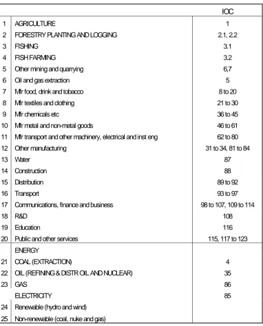
Both the Scottish and UK models share the some generic characteristics. There are 3 transactor groups, namely households, corporations, and government; 25 commodities and activities, 5 of which are energy commodities/supply (see Figure 1 and Tables 1 and 2 for details). The specific sectoral breakdown of the two models has been based on policy priorities and key energy use sectors in Scotland and the UK respectively. However, both models have the same 5 energy supply sectors: coal; oil; gas; renewable and non-renewable electricity (see Tables 1 and 2). Scotland is modelled as a region of the UK, with 2 exogenous external transactors, the Rest of the UK (RUK) and the Rest of the World (ROW). Separately identified is a third sub-set of these two – tourists (from RUK and ROW) who consume within the Scottish economy (see Section 5 – separate identification of this group in the Scottish IO tables is important as their consumption of energy will be officially counted as part of Scotland’s total energy consumption in the base year). The UK is modelled as a small open national economy, with a single exogenous external transactor, ROW. Tourist expenditure is not separately identified in the UK base year dataset (which incorporates the UK input-output accounts), so we are unable to distinguish this type of consumption in the model.
The generic AMOSENVI framework allows a high degree of flexibility in the choice of key parameter values and model closures. However, a crucial characteristic of the model is that, no matter how it is configured, we impose cost minimisation in production with multi-level production functions, generally of a CES form but with Leontief and Cobb-Douglas being available as special cases (see Figure 1). There are four major components of final demand: consumption, investment, government expenditure and exports. Of these, in the current application, real government expenditure is taken to be exogenous. Consumption is a linear homogeneous function of real disposable income. The external regions (RUK and ROW in the Scottish case, and ROW in the UK case) are exogenous, but the demand for domestic exports and imports is sensitive to changes in relative prices between (endogenous) domestic and (exogenous) external prices (Armington, 1969). Investment is a little more complex as we discuss below.
In both models, we impose a single local labour market characterised by perfect sectoral mobility. Wages are determined via a bargained real wage function in which the real consumption wage is directly related to workers’ bargaining power, and therefore inversely to the unemployment rate (Blanchflower and Oswald, 1994; Minford et al, 1994). Here, we parameterise the bargaining function from the econometric work reported by Layard et al (1991):
(8) wL,t = α- 0.068u + 0.40wL L,t-1
where: wL and uL are the natural logarithms of the local (Scottish or UK) real consumption wage and the unemployment rate respectively, t is the time subscript and α is a calibrated parameter.1 Empirical support for this “wage curve” specification is now widespread, even in a regional context (Blanchflower and Oswald, 1994).
Within each period of the multi-period simulations using the AMOSENVI framework, both the total capital stock and its sectoral composition are fixed, and commodity markets clear continuously. Each sector's capital stock is updated between
1 Parameter α is calibrated so as to replicate the base period, as is β in equation (9). These calibrated
parameters play no part in determining the sensitivity of the endogenous variables to exogenous
periods via a simple capital stock adjustment procedure, according to which investment equals depreciation plus some fraction of the gap between the desired and actual capital stock. The desired capital stock is determined on cost-minimisation criteria and the actual stock reflects last period's stock, adjusted for depreciation and gross investment. The economy is assumed initially to be in long-run equilibrium, where desired and actual capital stocks are equal.2
In the Scottish model, where endogenous migration is incorporated in the model (i.e. labour can freely migrate from the rest of the UK; in contrast to the UK, where there are restrictions on migration from ROW), population is also updated between periods. We take net migration to be positively related to the real wage differential and negatively related to the unemployment rate differential between Scotland and RUK, in accordance with the econometrically estimated model reported in Layard et al (1991). This model is based on that in Harris and Todaro (1970), and is commonly employed in studies of US migration (e.g. Greenwood et al, 1991; Treyz et al, 1993). The migration function we adopt in SCOTENVI is therefore of the form:
(9) m =β- 0.08 u - u + 0.06 w - w
(
s r)
(
s r)
where: m is the net in-migration rate (as a proportion of the indigenous population); wr and ur are the natural logarithms of the RUK real consumption wage and unemployment rates, respectively, and β is a calibrated parameter. In the multiperiod simulations reported below the net migration flows in any period are used to update population at the beginning of the next period, in a manner analogous to the updating of the capital stocks. The regional economy is initially assumed to have zero net migration and ultimately net migration flows re-establish this population equilibrium.
3.2 Treatment of energy inputs to production
Figure 1 summarises the production structure of the generic AMOSENVI framework. This separation of different types of energy and non-energy inputs in the intermediates block is in line with the general ‘KLEM’ (capital-labour-energy-materials) approach that is most commonly adopted in the literature. There is currently no consensus on precisely where in the production structure energy should be introduced, for example, within the primary inputs nest, most commonly combining with capital (e.g. Bergman, 1988, Bergman, 1990), or within the intermediates nest (e.g. Beauséjour et al, 1995). Given that energy is a produced input, it seems most natural to position it with the other intermediates, and this is the approach we adopt here. However, any particular placing of the energy input in a nested production function restricts the nature of the substitution possibilities between other inputs. The empirical importance of this choice is an issue
2 Our treatment is wholly consistent with sectoral investment being determined by the relationship
that requires more detailed research, and will be the subject of future research in the current research programme (see Section 6).3
The multi-level production functions in Figure 1 are generally of constant elasticity of substitution (CES) form, so there is input substitution in response to relative price changes, but with Leontief and Cobb-Douglas (CD) available as special cases. In the applications reported below for both Scotland and the UK, Leontief functions are specified at two levels of the hierarchy in each sector – the production of the non-oil composite and the non-energy composite – because of the presence of zeros in the base year data on some inputs within these composites. CES functions are specified at all other levels.
At present, econometric estimates of key parameter values are not available for either the Scottish or UK models (again this will be the focus of future research, with one aim of the sensitivity analysis reported being the identification key priorities for econometric work – see Section 6). In the base case scenario simulations reported in Section 4, we assume that the elasticity of substitution at all points in the multi-level production function takes the value of 0.3, apart from where Leontief functions have been imposed and in the case of the electricity composite, where we assume a value of 5.0 (to reflect the homogeneity of electricity from different sources and consequent higher degree of substitutability). The Armington trade elasticities are set universally at 2.0, with the exception of exports of renewable and non-renewable electricity, which are set at 5.0, again to reflect the homogeneity of electricity as a commodity in use.
We introduce the energy efficiency shock by increasing the productivity of the energy composite in the production structure of all industries. This procedure operates exactly as in equation (1). It is energy augmenting technical change. We do not change the efficiency with which energy is used in the household or government consumption, investment, tourism (in the case of Scotland) or export final demand sectors. Moreover, note that under the current production structure in Figure 1, we are only able to apply the efficiency shock to use of local energy, and not imports. This is an important limitation (see Section 5.4) and one that we aim to address in future research.
3.3. Databases
The database on which the structural characteristics of the Scottish model are calibrated is a social accounting matrix (SAM) for 1999. The core element of the Scottish SAM is the published Scottish input-output (IO) tables for 1999 (Scottish Executive, 2002). 1999 has been retained as the base year for the SCOTENVI model because the sectoral breakdown of this particular IO database separately identifies sectors of central importance in assessing the likely impact of energy efficiency. This allows us to
3 Note that there is also debate in the CGE literature regarding the use of nested functional forms because
distinguish among four broad energy types: coal, oil, gas and electricity. In particular, we have been able to draw on experimental data supplied by the input–output team at the Scottish Government to disaggregate the electricity supply sector into the ‘Renewable (hydro and wind)’ and ‘Nonrenewable (coal, nuclear and gas)’ sectors. However, we hope that a more updated variant of this database will be available in future. The reader is referred to Hanley et al (2008) for a more extensive discussion of the SCOTENVI SAM.
The main database for UKENVI is a specially constructed SAM for the UK economy for the year 2000. This required the initial construction of an appropriate UK Input-Output (IO) table since an official UK analytical table has not been published since the 1995 table in 2002 (National Statistics, 2002). A twenty-five sector SAM was then developed for the UK using the estimated IO table as a major input. The sectoral aggregation is chosen to focus on key energy use and supply sectors. The division of the electricity sector between renewable and non-renewable generation used the experimental disaggregation provided for Scotland. This was then adjusted to reflect the different pattern in electricity generation between the UK and Scotland. Full details on the construction of the UK IO table and SAM are provided in Allan et al (2006).
4. Impacts of an increase in energy efficiency in the Scottish and UK economies: base case scenario
4.1 Simulation strategy and calculation of rebound effects
In this Section we present the results from simulations of an illustrative 5% exogenous (and costless4) increase in energy efficiency in all production sectors in both the Scottish and UK models where both the production and trade parameters are specified as outlined in Section 3.2 for the base case scenario. This shock is a one-off step increase in technical efficiency, imposed as an energy-augmenting change to the energy composite. That is to say, in each industry there is a 5% increase in the efficiency with which the energy composite combines with the non-energy composite to produce the local intermediate composite input (see Figure 1).
Intermediate inputs of locally supplied energy account for 72.6% of total Scottish demand for electricity and 47.3% of the demand for non-electricity energy which give the corresponding values for α when equation (7) is used to calculate rebound effects (the implication is that the 5% energy efficiency shock in production equates to a shock affecting 3.63% of total electricity use and 2.37% of non-electricity energy use). In the UK the shares of electricity and non-electricity energy demand affected are 69.2% and 59.4% respectively so that the denominator of (7) is 3.46% in calculating the electricity rebound effect and 2.97% in calculating the non-electricity rebound effect.
When the efficiency improvement is introduced to the SCOTENVI and UKENVI models, the resulting changes in key energy and economic variables are
4 Introducing consideration of costs involved in introducing an energy efficiency improvement will affect
reported in terms of the percentage change from the base year values given by the 1999 Scottish SAM and 2000 UK SAM respectively. In both cases, the economy is taken to be in long-run equilibrium prior to the energy efficiency improvement, so that when each model is run forward in the absence of any disturbance it simply replicates the base year dataset in each period. The reported results refer to percentage changes in the endogenous variables relative to this unchanging equilibrium. All of the effects reported in each case are directly attributable, therefore, to the stimulus to energy efficiency.
4.2 Simulation results – base case scenario
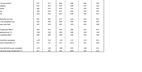
The first four columns in Table 3 report the impacts on key aggregate variables for the central case scenario for the UK and Scotland respectively. Here, the efficiency change is introduced costlessly5 and the default model configuration and parameter values are used (see Section 3.2). The figures reported are percentage changes from the base year values. Because the economy is taken to be in full (long-run) equilibrium prior to the energy efficiency improvement, the results are best interpreted as being the proportionate changes over and above what would have happened, ceteris paribus, without the efficiency shock. The short and long run time periods in Table 3 are conceptual time periods. In the short-run (the first period after the shock), both labour (population) and capital stocks are assumed to be fixed at the level of individual sectors. In the ‘long run’ in both cases capital stocks have full adjusted fully to their desired sectoral values, and, in the case of Scotland, where migration from the rest of the UK occurs endogenously (see equation 9 in Section 3.1), population stocks also. For comparative purposes, the last two columns of Table 3 show the results for Scotland for the same simulation with no migration (so that the configuration of the two models is identical). If the reader compares these throughout the discussion below, the main point to note is that the long-run stimulus to the Scottish economy is smaller with no migration. The main underlying factor is that, without migration, real wages do not adjust back to their base year levels in the long run, with a sustained increase in nominal wages (which limits the competitiveness of the economy and, therefore, the effects of the positive supply shock). However, the key results in terms of energy consumption and the presence of long run backfire effect are not qualitatively different.
Where we run the model in period-by-period mode with the gradual updating of population (in the case of Scotland) and capital stocks, a close adjustment to the long run values will often take a number of years. In the case of the UK, for this particular shock (and base scenario specification), the model begins to converge on long-run values after around 25 years, but in the case of Scotland, it takes much longer. Indeed after 150 years (taken as a proxy for long-run equilibrium in Table 3), convergence is very close but not entirely complete on all variables. This is due to the much greater stimulus to the Scottish economy from this shock, as explained below.
With wage determination characterised by a bargained wage curve, a beneficial supply-side policy, such as an improvement in energy efficiency, increases employment, reduces the unemployment rate and increase real wages. This has a positive impact on UK economic activity that is generally greater in the long run than in the short run (with the exception of household consumption). In the long run there is an increase of 0.17% in GDP, 0.21% in employment and 0.22% in exports. The expansion
is lower in the short run, where GDP increases by 0.11%, where there is a larger increase in consumption but actually a fall in exports. There is also a drop in imports. The net effect on imports depends on the strength of the relative price effect (as UK prices fall, imports to production and final consumption activities will fall in favour of locally produced goods) and the stimulus generated by increased economic activity (which will increase UK demand for all local and imported commodities). In the first column of Table 3 the former effect dominates and imports decrease.
This is in contrast with the Scottish case. Here the short-run stimulus to GDP, employment, real wages and consumption is proportionately smaller than in the UK, but there is an immediate increase in exports. Note also that the proportionate increase in aggregate investment demand is greater in Scotland (a point we return to below). In the long run (or after 150 periods), note that all of the positive effects of the increase in energy efficiency are greater than in the UK case. To consider why the effects of this particular positive supply shock are different in the Scottish and UK cases, let us begin by looking at the impact on sectoral output prices.
Figure 2 shows the short and long run impacts on Scottish output prices. For each sector this will reflect the net effect of changes in costs of production (capital rental rates, nominal wages, price of energy and non-energy intermediates) as well as the demand-side response. Figure 2 shows that, while output prices generally fall across the board, in some sectors the price rises initially (due to the increased price of labour and capital rental rates while capacity is constrained). The largest fall in output prices is observed in the more energy-intensive energy supply sectors. Note that what is happening here is, since we have local production of energy, actual as well as effective energy prices fall (as discussed in Section 2.2). As explained at the start of Section 3, the system-wide response to the drop in both effective and actual energy prices acts to offset the engineering or pure efficiency effect of the initial disturbance. However, the net effect on the five energy supply sectors varies in the short run. Figure 3 shows that the output of the three Scottish non-electricity energy supply sectors falls in the short run as less energy is required in the production of output in other sectors. That is, while final consumption of oil, coal and gas rises as prices fall, the efficiency effect that is taking place in intermediate demand dominates in the short run. The output of the two electricity sectors, on the other hand rises from the outset. Again, intermediate demand for Scottish electricity falls. However, the competitiveness effect dominates here, as increased export demand (combined with increased household demand) is sufficient to offset the fall in intermediate demand. In the long run, as local energy prices drop further, the combination of substitution, composition, competitiveness and income effects dominate and output increases in all of the Scottish energy supply sectors.
The effects in the UK are somewhat different. Figure 4 shows a similar qualitative pattern in terms of output prices; however, note that the percentage fall in the price of output in the UK energy supply sectors is generally larger than that observed in Figure 2 for the corresponding Scottish sectors. This is partly explained by the fact that (according to our IO databases6) the UK energy supply sectors are themselves generally (but not entirely) more energy intensive than the corresponding Scottish sectors. This is particularly the case with respect to the UK electricity supply sectors. In Figure 2 we see a huge drop in short run output prices, particularly in the two electricity sectors. As in the case of Scotland, the fall in local energy prices does stimulate export demand. However, the crucial point is that, with the exception of the ‘Oil (Refining and Distribution Oil and Nuclear)’ sector the initial level of energy exports is very low in
6 It is important to bear in mind the limitations of the UK IO database in particular, as outlined in Section
the UK (see Table 4). As a result, the positive competitiveness effects are of little importance relative to the efficiency effect in the short-run. However, the extreme drop in prices, particularly in the electricity supply sectors, has another important effect (one that is observed in Scotland in the non-electricity energy supply sectors, but to a much lesser extent). This is that profitability is reduced to a sufficient extent as to stimulate
disinvestmentin the energy supply sectors. The return on capital falls in all of the UK energy sectors (which tend to be relatively capital-intensive) and, as reinvestment begins (in response to growth in domestic demand as the economy expands) the price of output has to begin rising again (see Figure 6). This will in turn limit the size of the substitution, composition, output and income effects that drive rebound effects as the economy adjusts. For this reason, note from the second column of Table 3 that the drop in both electricity and non-electricity consumption are larger and the associated rebound effects are smaller in the long run that they are in the short run. This is in contrast with Saunder’s (2008) argument that the long-run rebound effect will always be bigger than the short-run rebound effect because capital (and labour) are fixed in the short-run (constraining the rebound effect), but thereafter investment will occur (in response to increased marginal productivity of all factors as efficiency improves), expanding the space of production possibilities. Here this prediction does not hold because the reduction in profitability as output prices fall in energy supply sectors (particularly electricity supply) causes a sufficient drop in capital rental rates to stimulate disinvestment (a contraction in capacity) in these sectors, which in turn constrains the long-run rebound effect.
The time path of adjustment in total UK electricity and non-electricity energy consumption (which gives us the numerator in the rebound calculation in equation 7) is shown in Figure 8. Observe that, apart from some minor upward adjustment, the long-run fall in energy consumption is achieved fairly rapidly, after around 15-20 years. However, throughout the period the fall in either type of energy consumption remains smaller than the effective efficiency improvement (determined by the share of energy consumption affected by the efficiency improvement – 3.46% in the case of electricity and 2.97% for non-electricity).
In contrast, in the Scottish case, while a disinvestment effect is observed to some extent in the Oil (Refining and Distribution Oil and Nuclear)’ and ‘Gas’ sectors, this corrects fairly quickly, and a continuing drop in prices is observed (to a lesser or greater extent) in all 5 energy supply sectors (see Figure 7). The result of this is that further impetus is given to the substitution, composition, competitiveness, and income effects that drive rebound effects as the economy adjusts. The most striking feature of the Scottish results is the reported strength of rebound effects. In the short run total electricity and other, non-electricity, energy consumption do fall, but only by 1.33% and 1.08% respectively in the face of the 5% stimulus to energy efficiency (which equates to 3.63% and 2.37% respectively in the denominator of equation 7, given the boundaries of the shock).7 This results in relatively large rebound effects of over 63% and 54% for electricity and non-electricity energy respectively. In the long-run energy demands actually increase, so that backfire is present (a rebound effect of 131.6% in electricity
7 Note that in the Scottish case the ranking of rebound effects across electricity and non-electricity
and 134% in non-electricity energy consumption). Thus, while energy efficiency does initially lower the demand for energy, the increase in competitiveness is concentrated in the most energy-intensive sectors of the economy. Where a sector is also a large exporters, this generates a significant boost to that sector and to the economy as a whole.
The impacts on the adjustment path of total energy consumption in Scotland in Figure 8 are striking. While the total amount of electricity consumed in Scotland initially falls, by period 14 it has risen above the base year value so that rebound becomes backfire. Non-electricity energy consumption follows a similar pattern, with the rise above the base year value occurring two years later (in period 16).
Thus, we have two key contrasts between the rebound results for Scotland and the UK in our base case scenario. First, rebound effects are bigger in Scotland than in the UK, to the extent we observe the extreme case of backfire in the Scottish case. Second, the time path of adjustment is different, with rebound bigger in the short-run in the UK while the reverse is observed in Scotland. Both outcomes have a common driver: falling actual (as well as implicit) energy prices. In the case of Scotland, this stimulates export demand (particularly for the outputs of the Scottish energy supply sectors) to the extent that output (competitiveness) effects dominate. In the case of the UK, export demand is also stimulated, but the absolute size of the output effect (due to the relative lack of trade in energy) is not sufficient to offset another key effect: falling prices in the energy supply sectors reduce profitability to such an extent that there is a disinvestment effect.
5. Sensitivity analysis
5.1. Simulation strategy for sensitivity analysis
that rebound effects will occur even where key elasticities of substitution in production are set close to zero, our intention is to investigate just how much price sensitivity in production and/or trade is required to induce the type of results observed so far. Therefore, this section of this paper is devoted to carrying out a systematic sensitivity analysis, where we gradually introduce and increase relative price sensitivity to the production and trade parameters of both the Scottish and UK models.
For each case we have carried out the matrix of simulations shown in Table 5 with all parameters in production varied as shown in the rows and all trade parameters (imports and exports) in both production and final consumption varied as shown in the columns. We have run these as multi-period simulations, with Tables 6 and 7 reporting the short run (first period/year after the shock) and long run (taken as period 1508) results. Note that our intention was to use Leontief functional forms to represent the case of zero elasticity and Cobb Douglas to represent unitary elasticity (CES is unstable with an elasticity values of 0 and 1). However, our initial simulation runs in these cases (with the exception of Cobb Douglas for the trade parameters) either would not solve or gave results with huge backfire effects where these would not be expected (this may reflect the arguments put by Saunders, 2008, regarding appropriate functional forms for estimating rebound in a partial equilibrium context). Therefore, as indicated in Table 5 for the zero elasticity/Leontief case, we have instead used CES with the smallest positive value that would allow the models to solve along the row (production) and down the column (trade).9 This value is 0.064. In the Cobb-Douglas/unitary elasticity case, we have used CES with the elasticity value set at 0.999999 in the case of production. However, we have retained Cobb-Douglas for unitary trade elasticities as this appears to give sensible results (Sanders’s, 2008, arguments about Cobb-Douglas resulting in unrealistically high rebound effects are only made in the case of production functions).
5.2.Overview of sensitivity results
The sensitivity of the rebound effect to varying the value of the production and trade elasticities is shown in Tables 6 and 7 for the Scottish and UK cases respectively. We discuss the results by examining whether a several of the observations made in the base case scenarios reported in Section 4 hold in all cases.
First of all, we noted that in the base case scenario the time path of rebound effects was different in Scotland and the UK, with rebound effects growing over time in Scotland, while the opposite was true in the UK case. If we consult Tables 6 and 7 we see that this is not a general result. The shaded cells in Tables 6 and 7 show cases where rebound is bigger in the short-run than in the long run, and this is observed in both Scotland and the UK. In Section 4, we concluded that this outcome (which is in contrast with the theoretical predictions of Saunders, 2008) occurs where there is a disinvestment effect in the energy supply sectors in response to the drop in output prices. The disinvestment effect does occur in most of the UK simulations reported in
8 As explained in Section 4.2, both models are converging on a long run solution (both labour and capital
stocks fully adjusted) by period 150, though, while the rebound effects have settled, convergence on all variables is not quite complete in all the Scottish simulations.
9 We retain Leontief technology in the two nests of the production function in Figure 1 – production of
Table 6, even where the rebound effect is bigger in the long than the short run (see below), only disappearing for some (but not all) sectors in the simulations reported in the last two columns of Table 7. It also occurs for Scotland, but in this case disappears entirely in the last five columns of Table 7. In both cases, as we read along each row (i.e. holding production elasticities constant while trade elasticities grow), the disinvestment effect lessens as trade (particularly export demand) becomes more price elastic (though import demand will also be important as, with external prices determined exogenously, increased substitution in favour of imports will limit the drop in output prices and profitability).
Recall that the disinvestment effect occurs because output prices in the energy supply sectors in particular (as the most energy intensive sectors) drop in response to the increase in energy efficiency. The lower the price elasticity of demand (due in Tables 6 and 7 to low Armington price elasticities of export demand and/or the initial level of external demand), price drops further and profitability falls so much that capital rental rates (the return on capital) collapse and disinvestment occurs. Where the trade parameters are set at less than 1, there are a number of cases where there is actually a negative terms of trade effect in both the Scottish and UK cases, with a decrease in GDP, employment and consumption (for example, Table 8 shows the short and long run GDP results for the UK and Scotland). In these case the increase in energy efficiency actually manifests itself as a negative supply shock due to the collapse in local energy supply prices (note that in the UK case, there are some simulations in Table 6 - marked with an asterix - where the negative supply effect is so extreme that the model fails to solve for a new equilibrium). This negative effect is greater the higher the production elasticities are set (i.e. as we read down the columns), because here the system responds to the drop in energy prices by using more energy in production throughout the economy, while the drop in output prices (i.e. the positive competitiveness effect) lessens the more elastic is intermediate demand for energy. Thus we observe very large rebound, and sometimes backfire, effects accompanying a contraction in aggregate economic activity.
In terms of the relative strength of short and long run effects (i.e. in the base case the disinvestment effect was associated with rebound effects that are bigger in the short run than in the long run), we also observe a reversal of this relationship in the presence of disinvestment in cases where inelastic trade parameters combine with more elastic production parameters. This reversal is again explained by what happens with prices and the impact on competitiveness in the short-run. In the non-shaded cells on the left of the grids in Tables 6 and 7 we observe cases where the long-run rebound effect is larger than in the short run in the presence of the disinvestment effect. As explained above, disinvestment constrains the long-run rebound effect. However, in the columns where trade parameters are set at low values, this means that export demand is highly inelastic, which in turn constrains the positive competitiveness and short-run rebound effect as well. As export demand becomes more elastic, the short-run rebound effect grows overtaking the growth of the long-run effect in the shaded area of the grid. This is slower to happen the higher the production parameter values as more elastic intermediate demand for energy limits the fall in prices that stimulates the competitiveness effect. This limits the short-run response in export demand, which in turn negatively impacts the positive supply side effects expected from an efficiency improvement (GDP falls as we read down the short run columns in Table 8) and limits the size of the short run rebound effect.
100%) does not occur in the UK case. However, examination of Table 6 again shows that this is not a general result. In Tables 6 and 7 we observe backfire effects for both Scotland and the UK, and, in a large number of cases, backfire effects actually occur in both the short and long run. However, in the UK simulations, the presence of backfire effects requires higher elasticities of substitution in production than in the Scottish case (where the trade in energy is more important and the trade parameters exert a greater influence). For both Scotland and the UK, the size of the rebound effect grows as we read down the columns for both electricity and non-electricity in Tables 6 and 7, and that the size of the rebound effect becomes more comparable across the two economies as we do so. Indeed, larger effects are observed for the UK when both production and trade parameters are highly elastic, and where production is highly inelastic (we focus on the latter case, where negative rebound effects are actually observed, in Section 5.4). The results would seem to support Allan et al’s (2007) conclusion regarding the relative importance of production parameters over trade parameters for the UK. This is explained by the fact that the UK is a national economy (encompassing the Scottish case), and is less open, particularly with respect to energy, both in terms of energy exports but also imports.
Another interesting result in Tables 6 and 7 is that backfire effects are not observed in the portions of the grids where both production and trade parameters are set at values of less than 1. Remember from our theoretical exposition in Section 2.1 that we note three important ranges of the general equilibrium price elasticity of demand for energy. There we noted that if this elasticity lies between zero and unity there would be a fall in energy use but some rebound effect, though not backfire, which would require that the general equilibrium price elasticity of demand for energy is greater than unity. The results in Tables 6 and 7 are consistent with this conclusion. However, the two sets of parameters examined in the sensitivity analysis do not tell the whole story. Indeed, to test this conclusion, additional simulations were run for Scotland with both sets of parameters set at 0.9 and backfire effects were observed in some cases, suggesting that other determinants of the general equilibrium price elasticity of energy demand are exerting an upward influence. In Section 2.2 we explained that these would include parameters determining the elasticity of supply of other inputs/factors and income elasticities of energy demand, which are not examined in the current sensitivity analysis.
5.3 Summary of initial sensitivity analysis
rapid. We also do not observe the change in direction of the energy consumption effects that leads to the switch between rebound and backfire effects observed in Figure 8. Examination of Table 7 shows that higher elasticities of substitution in the trade parameters are required for this type of effect to occur in Scotland. In both the UK and Scotland these patterns will also be observed where trade parameters are set very low while elasticities of production are highly inelastic. Figure 17 graphs the time path of adjustment for each of the cases in UK and Scotland where short run rebound and long run backfire are first observed as we raise production and trade parameters respectively. Note that in the Scottish case the most dramatic result is observed where trade parameters are highly elastic (against production elasticities of less than 0.1), while the opposite is true in the case of the UK, where elastic production elasticities give more variation in the path of adjustment (though, again, adjustment to long run equilibrium occurs relatively rapidly).
Figures 11 and 12 (UK) and Figures 15 and 16 (Scotland) illustrate the inflence of trade by holding all production parameters constant (also at unitary elasticity10) while varying price elasticities of import and export demand (increasing the openness of each economy to trade). Figures 11 and 12 illustrate that only when trade is highly inelastic in the UK do we observe larger rebound effects in the long run than in the short run. As trade also becomes elastic we observe backfire effects in both the short and long run, but the latter is constrained by the net disinvestment in the aggregate energy supply sector (this occurs in all of the UK simulations response to falling profitability as energy prices drop). Figures 15 and 16 illustrate the range of qualitative effects found in the Scottish case. When trade is highly inelastic (0.1) we see the expected pattern of bigger long-run than short-run rebound effects, but the limited competitiveness effects and the disinvestment effect combine to dampen the rebound effect over time. As trade becomes less inelastic (0.5 and 1.0) rebound effects grow throughout the period but are still constrained by the disinvestment that takes place after period 1. As the economy becomes more open, with more response through trade to the changes in local energy prices and the disinvesment effect disappears, rebound effects become backfire from the outset (given unitary elasticity of substitution in all production parameters) and grow over time.
5.4. Presence of ‘negative rebound’ effects
Another interesting result in Tables 6 and 7 for both Scotland and the UK is the apparent occurrence of negative rebound results. That is, proportionate decreases in total energy consumption that are greater than the proportionate increase in energy efficiency. Saunders (2008) discusses the possibility of ‘super-conservation’, which he explains is a counter-intuitive result (“How can, say, a 1% increase in fuel efficiency result in a 2% decline in fuel use?”, Saunders, 2008, p.20), but argues that such a result may arise the “host of complex interactions” (op cit) invoked by profit maximisation (or cost minimisation) in production. ‘Super conservation’ may be a misleading term in explaining how different system-wide (general equilibrium) responses to the effects of falling (actual and effective) energy prices may lead to further reductions in energy use. We have already seen that falling energy prices may in fact reduce profitability to such
10 Note from the discussion in Section 5.1 that for production functions we use CES with values of
an extent as to trigger disinvestment, which will act to constrain rebound effects. This is not an energy saving/conservation in response to the change in efficiency as such – it is a general equilibrium response to falling profitability, factor returns and incomes. In this section we explore what underlies the observations of negative rebound effects (in both the short and long run) in Tables 6 and 7.
In order to investigate more thoroughly, we revisit each of the simulations where negative rebound effects are observed in Tables 6 and 7 and consider factors that may explain their occurrence.
Treatment of imported energy
The first issue to consider is whether any problems with our model specification (and/or database) may be giving us distorted results. A clear candidate in this respect is the impact of including imported energy in our rebound calculations. From Section 4.1 and Figure 1 note that the energy efficiency shock is introduced at the level of the local energy composite, with the implication that use of imported energy is not affected. This is not a particularly realistic assumption, since it means that local producers only improve energy efficiency when using locally supplied energy as inputs to production and not imported energy. However, given the present production structure and specification of the model, it is not possible to target imported energy use (which comes in at a higher level of the production function) with the efficiency shock.
Nonetheless, imported energy is part of total energy consumption in the numerator of equation [7], and imports do in fact fall in all cases where negative rebound effects are observed. This will exert downward pressure on the size of the rebound effect. Therefore, our first additional test is to examine whether negative rebound effects are observed if we ignore consumption of imported energy in the calculation of [7].11
If we examine the case of Scotland first, Table 9 shows the rebound effect for Simulations 1-15 (the portion of the grid(s) in Table 7 where negative rebound effects are observed). The first thing to note is that the difference in results relative to those in Table 7 is bigger in the case of non-electricity energy consumption. This is because imports account for a larger share of non-electricity (28%) than electricity (0.4%) consumption in Scotland. As expected ignoring imports increases positive rebound effects and reduces negative rebound effects (for both types of energy use). Thus, we can conclude that the magnitude of the rebound effect is sensitive to the treatment of imported energy. The next question is whether the direction, or presence of the rebound effect is sensitive in this regard.
The entries highlighted in bold in Table 9 indicate the cases where negative rebound effects were observed in the initial simulations in Table 7. When use of imported energy is ignored, these disappear in several cases:
11 Note that the denominator of equation [7] also changes. When we ignore use of imported energy, in the
• In Simulation 3 (0.064 elasticity on production, 0.3 on trade), and Simulation 30 (0.3 on production, 0.1 on trade) the negative short run rebound effect on non-electricity energy consumption becomes positive.
• In Simulations 4 and 5 (0.064 elasticity on production, 0.5 and 0.8 respectively on trade) and Simulation 18 (0.1 on production, 0.5 on trade), the negative long run rebound effects on non-electricity energy consumption become positive. For the UK the results are much more dramatic in terms of the magnitude of the rebound effect. Table 10 shows the electricity rebound effects for all the successful simulations in the first four rows of the grid when consumption of imported energy is ignored (we have no non-electricity energy imports recorded in our database for the UK). The impact of ignoring imported energy (electricity) on the magnitude of the rebound effect is large relative to what is observed for Scotland. This is because imported electricity is relatively more important in the UK than Scotland (see Footnote 11). Indeed (momentarily turning our attention away from the issue of negative rebound) we now get one case of a short run backfire effect for the UK in the third row of the grid (where production elasticities are set to 0.3) and two in the fourth row (production elasticities set to 0.5), where previously these were not observed until the fifth row (production elasticities set to 0.8).
Turning our attention back to the direction of the rebound effect, again, the entries highlighted in bold in Table 10 indicate the cases where negative rebound effects were observed in the initial simulations in Table 6. Now, when we ignore imports from the calculation of the rebound effect, the negative short-run rebound effect disappears in all but one case, where the elasticities on trade and production are both set to 0.3 (the most constrained combination that the UK model was able to solve for). In the long run, the negative rebound effect disappears earlier as trade elasticities rise in each row. However, a number of long-run negative rebound effects remain, even where imports and exports are price elastic (i.e. greater than 1) in the first two rows of the grid (where production elasticities are set to zero or 0.1).
The implication of the direction of the rebound effect in some case, and its magnitude in all cases being sensitive to the treatment of imported energy in our Scottish and UK models (to a small extent in some cases, but a large extent in others) is that, alongside improving the quality of our trade data, a future research priority should be to adapt the production structure to allow use of both local and imported energy to be targeted with efficiency improvements. Moreover, imports will also be important in the case of efficiency improvements in consumption also. One approach (within the existing production structure and other alternatives outlined in Section 3.2) would be to specify the choice between local and imported inputs at the commodity level, at least in the case of energy commodities/services. Generally, the treatment of imported energy merits further research: in Turner (2002) we find that a crucial issue in the energy CGE literature is whether imported and domestic energy inputs should be treated as perfect substitutes or homogeneous products in some or all sectors.
Focus on the intermediate rebound effect (energy consumption in production)
‘super conservation’ effect) or whether other factors drive the observed negative rebound effects. Therefore, next we recalculate the rebound effects, this time removing final consumption of energy. This will allow us to examine the impact on the rebound effect of rising/falling incomes in the household sector. For example, Learmonth et al (2007) find that where very low elasticities of substitution in production combine with highly inelastic export demands, the direct and derived demand for labour falls to such an extent that energy use and pollution generation in the household sector actually decrease as output and employment rise in all sectors of the economy rise. This is a result of reduced real household income and expenditure.
In the case of Scotland, where tourist consumption is also identified within total energy consumption in the economy, final consumption was examined in stages, first examining the impact of removing energy use by tourists to focus on local energy consumption (households and production). However, energy consumption by tourists in Scotland (in our base year of 1999) is relatively unimportant, accounting for around half of 1% of total use of locally supplied energy for both electricity and non-electricity energy. As a result, the rebound results ignoring tourist were virtually unchanged from those reported in Table 9 (to 2 decimal places if at all) so we do not report them here. Household consumption of energy is much more important, both in Scotland (where, in our 1999 database) households accounted for just under 27% of local consumption (households and production) of locally supplied electricity and just under 34% of local consumption of locally supplied non-electricity energy outputs. For the UK (according to our 2000 database) the corresponding figures are 28% and 40.6% respectively. Tables 11 and 12 show the recalculated rebound effects for Scotland and the UK for the portions of the grids in Tables 9 and 10 where negative rebound effects were observed (i.e. here we continue to ignore use of imported energy).
In almost all cases where we see a drop in GDP in response to the energy efficiency improvement (Table 8), this is accompanied by a drop in real household income and total expenditure (except in the long-run in the UK, where household consumption recovers more rapidly (due to the rise in the real take-home wage in the absence of in-migration - see Table 3). However, due to the improvement in competitiveness of locally produced commodities (local prices drop relative to external prices in response to the efficiency improvements) consumption of domestic commodities actually rises in all cases in the UK and most cases in Scotland at the expense of imports. Therefore, if we ignore household consumption (and retain the focus on use of locally supplied energy), this tends to put downward pressure on the rebound effect, as shown if we compare Tables 9 and 11 for Scotland and 10 and 12 for the UK. Indeed in the UK case, several additional instances of negative rebound occur (for both electricity and non-electricity consumption, where trade elasticities are higher).
(leading to a bigger fall in real income and expenditure), the bigger the increase in the short run rebound effect when we remove household consumption (i.e. the largest negative rebound effect, where both production and trade parameters are set to 0.064, sees the biggest recovery). However, reading down the first column, it is not until production parameters are set to 0.3 (Simulation 29) that removing household actually offsets the negative rebound effect (for both electricity and non-electricity consumption). Thus, while household income and consumption effects offer some explanation for negative rebound effects in some cases, we are left with a number of observations of negative rebound, for which the explanation must lie in the production sectors.
Distinguishing between energy efficiency improvements in energy supply and non-energy supply (non-energy use) sectors
Hanley et al (2008) carry out sensitivity analysis in terms of which sectors the energy efficiency improvement actually takes place in. Table 3 shows long run backfire in the Scottish base scenario when all 25 production sectors are targeted with the shock. However, Hanley et al (2008) find that when they target only the energy supply sectors the rebound effect grows to just under 250% in the case of electricity and 244% in the case of non-electricity. On the other hand, when the shock is targeted only at the other 20 energy use sectors, the rebound effects fall to 41.4% and 34.8% respectively (from the base scenario results of 131.6% and 134%). The energy intensity of production in the energy supply sectors offers a partial explanation. However, there is also a key difference in that the disinvestment effect observed in the UK base case scenario (Section 4.2), but not in the Scottish case (when all 25 production sectors are shocked), does now occur in Scotland also (when only the 20 energy use sectors are targeted). This difference is demonstrated if we compare Figure 18, which shows the impact on energy prices in the base case scenario where only the energy use sectors are targeted with the shock, with Figure 7, where all sectors are targeted. Note that while energy prices do not drop by as in Figure 18, given the smaller competitiveness effect (a much smaller stimulus to RUK export demand for Scottish energy) these are is sufficient to trigger disinvestment in the energy supply sectors. Note also that Figure 18 shows a similar pattern to UK prices in Figure 6, in that local energy prices have to rise again to permit reinvestment, thereby dampening rebound effects.
Table 13 shows the results of similarly breaking down the UK base case scenario shock to distinguish between energy supply and non-energy supply sectors (this time including the rebound effect calculated both with and without imported energy use). As in the Scottish case, rebound effects are bigger when only the energy supply sectors are targeted (though, in contrast to the Scottish case, the disinvesment effect means that rebound effects are bigger in the short than long run). However, the third and fourth columns of Table 13 show a (previously hidden) negative rebound effect where only the energy use sectors are targeted.
effects already identified in Tables 7 and 9 (where use of imported energy is removed) when all 25 production sectors are targeted with the energy efficiency improvement. Negative rebound effects are observed for both types of energy consumption in both the short and long run. When we break down the shock, first targeting only Sectors 1-20 (energy use) then Sectors 21-25 (energy supply), note that while negative rebound effects occur in all cases in both simulations, these are bigger in columns 3 and 4 where the non-energy supply sectors are targeted. However, this is not due to additional energy conservation in the energy use sectors as a direct result of the change in efficiency itself. If we examine Figure 19, note that the short run drop in energy consumption is proportionately less than the 5% efficiency improvement in each of the 2o production sectors targeted with the shock. The exception is Construction, where both types of energy consumption drop by just over 5%. However, in the base year 50% of this sector’s output goes to capital formation, the demand for which falls immediately, by 0.96%, indicating the triggering of the disinvestment effect, which we will discuss momentarily.
The source of short-run negative rebound effect is what happens in the five energy supply sectors, which account for 20% of the short run reduction in local electricity use and 22% of the reduction in non-electricity energy use. There are several causes and effects of what happens in the energy supply sectors. First, there is a net decrease in demand for energy as an input to production in the other 20 energy use sectors, with the pure efficiency effect only slightly offset by positive substitution and competitiveness effects, given that intermediate and final demands are both highly price inelastic. Second, given the very inelastic direct and derived demand for labour, there is a decrease in real household income and expenditure, including expenditure on local (as well as imported) energy. Third, there are negative multiplier effects in the energy supply sectors themselves as these (relatively energy-intensive) sectors reduce their own intermediate demand for energy inputs in response to the demand contractions elsewhere in the economy. While export demand for Scottish energy does grow slightly in response to falling prices in the energy supply sectors, the net contraction in what is already very inelastic demand causes prices to drop proportionately more than output so that there is a decline in revenue and profitability. This causes capital rental rates to collapse in the relatively capital-intensive energy supply sectors, triggering the disinvestment effect, with the implication that the negative rebound effect continues into the long-run.