Decentralized and hierarchical control of robot manipulators

(1)

City, University of London Institutional Repository

Citation: Osman, J.H.S. (1991). Decentralized and hierarchical control of robot manipulators. (Unpublished Doctoral thesis, City University London)

This is the accepted version of the paper.

This version of the publication may differ from the final published version.

Permanent repository link: http://openaccess.city.ac.uk/7758/ Link to published version:

Copyright and reuse: City Research Online aims to make research outputs of City, University of London available to a wider audience. Copyright and Moral Rights remain with the author(s) and/or copyright holders. URLs from City Research Online may be freely distributed and linked to.

City Research Online: http://openaccess.city.ac.uk/ [email protected]

(2)

DECENTRALIZED AND HIERARCHICAL CONTROL

OF ROBOT MANIPULATORS

BY

JOHAIU HALIM SHAH OSMAN,

B.Sc. (Physics), M.Sc. (Elec. Eng.)

A THESIS SUBMITTED FOR THE DEGREE OF

DOCTOR OF PHILOSOPHY IN ENGINEEIUNG

CONTROL ENGINEEIUNG CENTRE SCHOOL OF ELECTIUCAL ENGINEEIUNG

AND APPLIED PHYSICS

CITY UNIVERSITY

(3)

(4)

8,

ia As State Variables 66 2.3.2 Third Order Actuator Model With 0, 0,

°

As State Variables 67 2.4 Integrated Dynamic Model Of Robot Manipulator 70

(5)

2.5 Dynamic 110del Of A Three dof Revolute Robot Manipulator 78

2.5.1 Dynamic Equation Of The Mechanical Linkage 78

2.5.2 Derivative Of The Mechanical Link Torque 85

2.5.3 Model Of The DC Motors 87

2.5.4 Integrated Model Of the Three dof Robot Manipulator 89

2.6 Conclusion 91

CHAPTER 3 ROBOT MANIPULATOR AS A LARGE SCALE

UNCERTAIN SYSTEM 93

3.1 Introduction 93

3.2 Decomposition Of Robot Manipulator 94

3.2.1 Decomposition Based On Integrated Model With Joint

Angle, Velocity And Current As State Variables 96

3.2.2 Decomposition Based On Integrated Model With Joint

Angle, Velocity And Acceleration As State Variables 98

3.3 Robot 11anipulator As An Uncertain Interconnected System 102

3.4 Application To A Three dof Robot Manipulator 108

3.5 Conclusion 112

CHAPTER 4 DECENTRALIZED TRACKING CONTROLLER

DESIGN FOR ROBOTIC MANIPULATORS 114

4.1 Introduction 114

4.2 Deterministic Control Of Uncertain Systems 115

4.2.1 Deterministic Control Approach Of Leitmann [1981]'

And Corless And Leitmann [1981] 116

4.2.2 Application Of A Deterministic Approach To Robot

11anipulator Control - An Overview

4.3 Problem Formulation

4.4 Decentralized Nonlinear Tracking Controller Design

-Local Approach

4.5 Simulation And Results

4.5.1 Trajectory Generation

4.5.2 Simulation Using Independent Joint Linear Control

118

119

124

134

135

(6)

4.5.3 Simulation Using Decentralized Nonlinear Local Control

Method 143

4.5.3.1 Effect Of Load Variation 151

4.5.3.2 Effect Of Varying The Value €i 159

4.5.3.3 Effect Of Varying The \Veighting Matrix

Q. _,

162

4.6 Conclusion 167

CHAPTER 5 DECENTRALIZED GLOBAL TRACKING CONTROLLER

DESIGN FOR ROBOT MANIPULATOR

5.1 Introduction

5.3 Decentralized Nonlinear Tracking Controller Design

- Global Approach

5.4 Simulation And Results

5.4.1 Comparison Between Local And Global Approach

5.4.2 Effect Of Load Variation

5.4.3 Effect Of Varying The Value €i

5.4.4 Effect Of Varying The Weighting Matrix

Q.

I

5.4.5 Comparison Between The Decentralized And A

Centralized Control :Method

5.5 Conclusion

CHAPTER 6 HIERARCHICAL CONTROL CONCEPT IN

ROBOTIC SYSTEM

6.1 Introduction

6.3 Hierarchical Control Structure - Method 1

6.3.1 Controller Design At The Lowest Level

Linear Feedback Control

6.3.2 Controller Design At The Upper Level

Deterministic Approach

6.4 Hierarchical Control Structure - Method 2

6.4.1 Controller Design At The Lowest Level

Deterministic Approach

(7)

6.4.2 Controller Design At The Upper Level -Deterministic Approach

6.4.3 Stability Of The Overall System 6.5 Simulation And Results

6.5.1 Implementation Of The First Hierarchical Control 11ethod

6.5.2 Implementation Of The Second Hierarchical Control Method 6.5.3 Effect Of Load Variation

6.5.4 Effect Of Structural Perturbation

6.5.5 Effect Of Varying The Sampling Interval At The Upper Level

6.5.6 Comparison Between The Proposed Control Methods

6.6 conclusion

CHAPTER 7 CONCLUSION AND SUGGESTIONS

7.1 Conclusion

7.2 Suggestions For Future Research

7.3 Concluding Remarks

APPENDIX A DENAVIT-HARTENBERG (D-H) NOTATION

AND TRANSFORMATION MATRIX

APPENDIX B EULER-LAGRANGE FORMULATION OF

MANIPULATOR LINKS DYNAMICS

APPENDIX C ROBOT MANIPULATOR COMPLETE MODEL

- A SURVEY

APPENDIX D DETAILED EXPRESSIONS OF THE INTEGRATED

DYNAMIC MODEL OF THE THREE DOF

REVOLUTE ROBOT MANIPULATOR

(8)

Table 2-1

Table 2-2

Table 5-1

Table 5-2

LIST OF TABLES

CHAPTER 2

Parameters Of The Three dof Robot Manipulator Linkage

Parameters Of The Actuators

CHAPTER 5

Different Sets Of €j And The Corresponding TJ

G

Different Values Of Q_j And The Corresponding TJ

G

Page

80

81

198

(9)

Figure 1.1

Figure 1.2

Figure 2.1

Figure 2.2

Figure 2.3

Figure 4.1

Figure 4.2

Figure 4.3

Figure 4.4

Figure 4.5

LIST OF FIGURES

CHAPTER 1

Robotic System Components

N dof Robot 11anipulator

CHAPTER 2

Schematic Diagram Of Armature Controlled Permanent

Ma.gnet DC 11otor

Diagram Of The ith 11anipulator Link Actuated By DC

11otor \\'ith Gear Train

Three dof Revolute Robot Manipulator

CHAPTER 4

Decentralized Control Of Robot Manipulator - Local

Approa.ch

Desired Joint Position Profile

Desired Joint Velocity Profile

Desired Joint Acceleration Profile

Joint Tracking Error Without Load Using Linear Control

Method

Page

41

45

63

64

79

126

137

138

(10)

Figure 4.6

Figure 4.7

Figure 4.8

Figure 4.9

Figure 4.10

Figure 4.11

Figure 4.12a

Figure 4.12b

Figure 4.13a

Figure 4.13b

Figure 4.14a

Figure 4.14h

Joint Tracking Error For 20 Kg. Load Using Linear

Controller

Position Tracking Responses For 10 Kg. Load Using

Decentralized Local Control 11ethod

Velocity Tracking Responses For 10 Kg. Load Using

Decentralized Local Control Method

Acceleration Tracking Responses For 10 Kg. Load Using

Position Tracking Error For 10 Kg. Load

Joint Control Inputs For 10 Kg. Load Using

Joint 1 Tracking Response Under Different Load Using

Joint 1 Tracking Error Under Different Load Using

Decentralized Local Control :Method

(11)

Figure 4.15a

Figure 4.15b

Figure 4.16a

Figure 4.16b

Figure 4.17a

Figure 4.17b

Figure 4.18

Figure 4.19

Figure 4.20

Figure 4.21

Figure 4.22

Joint 1 Velocity Response Under Different Load Csing

Joint 1 Acceleration Error Under Different Load Using

Joint 2 Velocity Response Under Different Load Using

Decentralized Local Control 11ethod

155

156

Decentralized Local Control Method 157

Control Inputs For 0 Kg. Load Using Decentralized Local

Control 11ethod 158

Control Inputs For 20 Kg. Load Using Decentralized Local

Control Method 158

Joint 1 Tracking Error For 10 Kg. Load For Different

Values Of Ei

Joint 3 Tracking Error For 10 Kg. Load For Different Values Of Ei

160

(12)

Figure 4.23

Figure 4.24

Figure 4.25

Figure 4.26

Figure 4.27

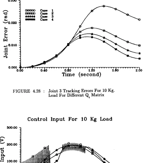
Figure 4.28

Figure 4.29

Figure 5.1

Figure 5.2a

Figure 5.2b

Figure 5.3a

Joint Control Inputs For 10 Kg. Load For (1

=

0.25 , f2

=

0.2 , f3

=

0.54

Joint Tracking Errors For 10 Kg. Load For (1

=

0.2 , f2

=

0.15 , f3

=

0.5

=

0.2 , f2

=

0.15 , f3

=

0.5

Q.

Matrix

I

Q.

Matrix

I

Q.

Matrix

I

Joint Control Inputs For 10 Kg. Load For

Q. =

1.1 13 I

CHAPTER 5

Decentralized Control Of Robot

:Manipulator-Global Approach

Joint 1 Tracking Response Under Decentralized Local

And Global Control Methods

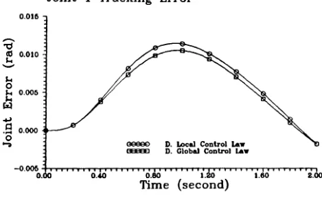
Joint 1 Tracking Error Under Decentralized Local And

Global Control Methods

(13)

Figure 5.3b

Figure 5.4a

Figure 5.4b

Figure 5.5

Figure 5.6

Figure 5.7

Figure 5.8a

Figure 5.8b

Figure 5.9a

Figure 5.9b

Figure 5.1 Oa

Decentralized Global Controller

185

186

187

Decentralized Global Control :Method 187

Joint Control Inputs For 10 Kg. Load Using Decentralized

Global Control Method 188

Decentralized Global Control Method 190

Decentralized Global Control Method

Decentralized Global Control :Method

Decentralized Global Control 11ethod

Decentralized Global Control Method

190

191

(14)

Figure 5.10b

Figure 5.11a

Figure 5.11b

Figure 5.12a

Figure 5.12b

Figure 5.13a

Figure 5.13b

Figure 5.14

Figure 5.15

Figure 5.16

Figure 5.17

Joint 3 Tracking Error Under Different Load LTsing

Decentralized Global Control :Method 194

Decentralized Global Control 11ethod 195

Control Inputs For 0 Kg. Load Using Decentralized Global

Control Method 197

Control Inputs For 20 Kg. Load Using Decentralized Global

Control 11ethod 197

Values Of fj

Joint 2 Tracking Error For 10 Kg. Load For Different Values Of fj

200

(15)

Figure 5.18

Figure 5.19

Figure 5.20

Figure 5.21

Figure 5.22

Figure 5.23

Figure 5.24

Figure 5.25

Figure 5.26

Figure 5.27

Figure 5.28

Figure 5.29

Values Of fi

=

0.6 , f2

=

0.3 , f3

=

0.7

Joint Tracking Errors For 10 Kg. Load For (1

=

0.4 , f2

=

0.15 , f3

=

0.5

=

0.4 , f2

=

0.3 , f3

=

0.5

Q. Matrix

I

Q.11atrix

I

Q.11atrix

I

Joint Control Inputs For 10 Kg. Load For Q.

=

1.1 13 I

Joint 1 Tracking Error Using Different Decentralized

And Centralized Control Methods

Joint 1 Tracking Error Using Different Decentralized And Centralized Control Methods

(16)

Figure 5.30

Figure 5.31

Figure 6.1

Figure 6.2

Figure 6.3

Figure 6.4

Figure 6.5

Figure 6.6

Figure 6.7

Figure 6.8

CHAPTER 6

Decentralized Linear Controller For The ith Decoupled

213

214

Subsystem At The Lowest Level Using Method 1 223

Two - Level Hierarchical Control Of Robot :Manipulator

- Method 1 226

Decentralized Nonlinear Controller For The ith Decoupled

Subsystem At The Lowest Level Using Method 2 229

Two - Level Hierarchical Control Of Robot Manipulator

- :Method 2 237

Hierarchical Control- Method 1 240

Position Tracking Error For 10 Kg. Load Using

Hierarchical Control-11ethod 1

Hierarchical Control- Method 1

Hierarchical Control-11ethod 1

240

241

(17)

Figure 6.9

Figure 6.10

Figure 6.11

Figure 6.12

Figure 6.13

Figure 6.14

Figure 6.15a

Figure 6.15b

Figure 6.16a

Figure 6.16b

Figure 6.17a

Joint Control Inputs For 10 Kg. Load Using Hierarchical Control- Method 1

Position Tracking Error For 10 Kg. Load Using

Acceleration Tracking Responses For 10 Kg. Load Using Hierarchical Control- Method 2

Joint Control Inputs For 10 Kg. Load Using Hierarchical

Control- Method 2

Hierarchical Control- :Method 1

(18)

Figure 6.1 7b

Figure 6.18

Figure 6.19

Figure 6.20a

Figure 6.20b

Figure 6.21a

Figure 6.21 b

Figure 6.22a

Figure 6.22b

Figure 6.23

Figure 6.24

Control Inputs For 0 Kg. Load Using Hierarchical Control

250

- :Method 1 251

- Method 1 251

Hierarchical Control- Method 2 252

Joint 3 Tracking Error Under Different Load Using Hierarchical Control-11ethod 2

252

253

254

- 11ethod 2 255

(19)

Figure 6.25

Figure 6.26

Figure 6.27

Figure 6.28

Figure 6.29

Figure 6.30

Figure 6.31

Figure 6.32

Figure 6.33

Figure 6.34a

Figure 6.34b

Joint 1 Tracking Error Under Different Structural

Perturbation For Hierarchical Control- Method 1

Perturbation For Hierarchical Control-11ethod 2

257

258

259

Perturbation For Hierarchical Control- Method 2 259

Joint 1 Tracking Error Under Different Rates Of

Computation Of The Coordinator - Method 1 261

Velocity Tracking Response When The Sampling Rate Of

The Coordinator Is At 0.05s - Method 1 263

Acceleration Tracking Response When The Sampling Rate

(20)

Figure 6.35a

Figure 6.35b

Figure 6.36

Figure 6.37

Figure 6.38

Figure 6.39

Figure 6.40

Figure 6.41

Figure 6.42

Figure 6.43

Figure 6.44

Velocity Tracking Response When The Sampling Rate Of

The Coordinator Is At O.ls - Method 1 264

Acceleration Tracking Response When The Sampling Rate

Of The Coordinator Is At O.ls - Method 1 264

Joint Control Inputs When The Sampling Rate Of The Coordinator Is At 0.05s - Method 1

Joint Control Inputs When The Sampling Rate Of The Coordinator Is At O.ls - Method 1

Computation Of The Coordinator - Method 2

Computation Of The Coordinator - :Method 2

Joint 1 Velocity Response Under Different Rates Of

Con1putation Of The Coordinator - Method 2

Joint 1 Acceleration Response Under Different Rates

Of Computation Of The Coordinator -11ethod 2

265

266

267

268

(21)

Figure 6.45

Figure 6.46

Figure 6.47

Figure 6.48

Figure 6.49

Figure 6.50

Figure 6.51

Figure A.l

Of Computation Of The Coordinator - ~lethod 2

Of Computation Of The Coordinator - Method 2

Joint Control Inputs When The Sampling Rate Of The Coordinator Is At 0.05s - :Method 2

Joint Control Inputs When The Sampling Rate Of The Coordinator Is At O.ls - Method 2

Joint 1 Tracking Errors Using Decentralized, Hierarchical,

269

270

271

And Centralized Control Methods 274

APPENDIX A

Denavit-Hartenberg Frame Assignment [Spong and

(22)

ACKNOWLEDGEMENTS

I would like to express my thanks and gratitude to my supernsor,

Professor P. D. Roberts, for his invaluable guidance, patience, and encouragement

throughout this project.

I would like to thank the Vniversiti Teknologi of Malaysia (V.T.1L) for

supporting this research in the form of a scholarship. There are many people at

V.T.M., amongst them Associate Professor Dr. Mohammad Nor Bin Salleh, to

whom lowe thanks for helping me secure the scholarship.

11y thanks are also due to Mrs. J. Rivellini, Iman Kartowisastro, and

other staff at the Control Engineering Centre for their help.

I would also like to thank my parents for their enduring patience,

understanding, and for taking care of my children, Izzaz and N adira.

Finally, I would like to express my utmost appreciation to my wife for her

constant moral support, encouragement and help, and to my daughter Yazmin,

(23)

DECLARATION

The author grants powers of discretion to the University Librarian to allow

this thesis to be copied in whole or in part without further reference to him. This

permission covers only single copies made for study purposes, subject to normal

(24)

PUBLICATION

The following paper, based on the work described in this thesis, has been

published:

1. Osman, J. H. S., and Roberts, P. D. [1991]: A Class Of Decentralized Tracking Controller For Robot Manipulators. Proc. Inst. Mech.

(25)

ABSTRACT

This thesis deals with the decentralized and hierarchical control of a class of robot manipulators, where the robot manipulator is treated as a large scale uncertain systelll. The work is divided into three parts.

The first part is concerned with the development of an integrated

mathematical model of the robot manipulator. The model of the system

considered comprises the mechanical part of the robot manipulator, the actuators, as well as the gear trains. The formulation results in nonlinear time varying state equations, which represent a more realistic model of the robotic system. A procedure to decompose and reduce the integrated model of the robot manipulator into a set of interconnected subsystems with bounded uncertainties description is then presented.

In the second part of the research, two decentralized control approaches based on a deterministic approach are outlined. The first method uses only the local states as the feedback information. It is shown that the robot manipulator utilizing the proposed controller is practically stable and tracks a reference trajectory if a given sufficient condition is satisfied. In the second approach, the controller is designed based on the local states as well as the states of the

neighbouring subsystems as the feedback information. It is shown that the

controller will force the nonlinear uncertain robot manipulator to track a desired trajectory to within a small uniform ultimate boundedness set.

In the final part of the study, two hierarchical control concepts for robot

manipulator are proposed. The controllers are formulated based on a

deterministic approach. It is shown that the hierarchical control strategies are capable of withstanding the expected variations and uncertainties and will render the robot manipulator to track a prescribed trajectory satisfactorily.

In synthesizing the proposed controllers, it is assumed that the upper bounds on the nonlinearities, couplings and uncertainties present in the system are available. The proposed methods are simple and robust to parameter variations and uncertainties present in the system. The performance of the proposed control

algorithms are evaluated by means of computer simulations. The proposed

control laws are applied to a three degree of freedom revolute robot manipulator

actuated by DC motors. Several case studies have been considered, and the

simulation results are presented and discussed.

In this thesis, the term practical stability means bounded stability in the

(26)

SYMBOL

1. Upper Case:

A(

*,*,*)

Aj( *,.,*)

LIST OF SYMBOLS

DESCRIPTION

3Nx3N system matrix for the integrated robot manipulator model

using OJ,

OJ,

and iaj as the state variables

ijth submatrix of AA( *,*,*)

system matrix for the ith subsystem

interconnection matrix between the ith and jth subsystems

3Nx3N system matrix for the augmented dynamic equation of the

actuators using OJ,

OJ,

and iaj as the state variables

3x3 system matrix for the ith actuators using OJ, OJ, and iaj as the

state variables

3Nx3N system matrix for the integrated robot manipulator model

using OJ,

OJ,

and OJ as the state variables

ijth submatrix of A_B(*,*,*)

3Nx3N system matrix for the augmented dynanlic equation of the

(27)

A· a

ApI (.,.,.)

Ap2( .,.,.)

'"V

A· a

B( .,.,.)

B B( .,.,-)

3x3 system matrix for the ith actuators using Oa.

B

_{i .}and

8

_i as the state variables

nominal system matrix for the ith subsystem

2Nx2N system matrix for the mechanical linkage dynamics

expressed in state state variable form

NxN matrix component of the matrix Ap( .,.,.)

closed loop system matrix for the ith subsystem

matrix representing the uncertainties in the system matrix for the

ith subsystem

Denavit-Hartenberg transformation matrix relating the ith

coordinate frame to the i-lth coordinate frame

3NxN input matrix for the integrated robot manipulator model

3NxN input matrix for the augmented dynamic equation of the

actuators using OJ,

B

_{i ,}and iaj as the state variables

3xI input matrix for the ith actuators using 0i,

B

_{i, and iai as the} state variables

3NxN input matrix for the integrated robot manipulator model

using 0i, 0i' and 0i as the state variables

(28)

B· 1

ID(7])

C(

*,*,*)

f"V

C ..

_{I )}

D( *,*,*)

D( *,*)

D ..

I )

D( .,.)

3NxN input matrix for the augmented dynamic equation of the

actuators using 8_{i ,}

ili,

and Bi as the state variables

3xl input matrix for the ith actuators using 0i, 8., and O. as the

state variables

input matrix for the ith subsystem

nominal input matrix for the ith subsystem

matrix representing the uncertainties in the input matrix for the

ith subsystem

2NxN input matrix for the mechanical linkage dynamics

expressed in state variable form

Penrose-Pseudoinverse of Bp( *,*,*)

viscous friction coefficient for the ith motor (Nm/rad/s)

close ball with radius 7]

NxN coefficient matrix related to the acceleration vector In the

derivative of the manipulator link dynamic equation

f"V

ijth element of the matrix C( *,*,.)

Nxl vector of Coriolis and centrifugal forces

N

Nx

L

i matrix related to D( *,*,*) vector

i = 1

ijth element of the matrix D( *,.)

(29)

D( *,*,*)

D(

*,*,*)

f'V

D·· I }

~.

I

G( *,*)

G· I

G(

*,*)

G( *,*)

NxN matrix related to D( *,*,*) vector

NxN coefficient matrix related to the velocity vector In the

derivative of the manipulator link dynamic equation

f'V

ijth element of the matrix D( *,*,*)

a continuous function related to ..1B_{I (}*,*)

back emf for the ith actuator

3NxN load distribution matrix for the augmented dynamic

equation of the actuators using B_{i, 0i, and iai as the state variables}

3xl load distribution matrix for the ith actuators using B_{i, 0i, and}

iai as the state variables

3NxN load distribution matrix for the augmented dynamic

equation of the actuators using B_i,

0i,

and

0

i as the state variables

3xl load distribution matrix for the ith actuators using BI , BI , and

o

i as the state variables

Nxl vector of gravitational forces

ith component of the matrix G( *,*)

derivative of G( *,*) with respect to time

NxN matrix related to the vector of gravitational forces G( *.*)

lx3 vector of continuous functions related to the interconnection

(30)

I· _l

J. _I

K· I

9G(.,.)

L( .,.)

L· I

1

M( *,.)

M·· I ]

M( *,*)

lx3 vector of continuous functions related to LlAj ( *,*)

an ixi identity matrix

moment of inertia at the centre of gravity for the ith link with

respect to x-, y-, and z-axis, respectively

set denoting the number of joint (degree of freedom) of the

manipulator

moment of inertia for the ith motor ( Kgm2)

pseudo inertia matrix of the ith link

linear feedback gain matrix for the ith subsystem

total kinetic energy of the system

Lagrange function

armature inductance for the ith motor (H)

field inductance for the ith motor (H)

Lyapunov function

derivative of the Lyapunov function 1

NxN inertia matrix of the manipulator linkage

ijth elements of matrix 11( .,.)

(31)

N· I

N

0·· I )

p.

I

P

Q

R· I

~N

T(*)

inverse of the gear ratio (gear ratio=l/NJ for the ith joint

number of degree of freedom/joints of the robot manipulator

an ixj null matrix

solution of matrix Lyapunov equation for the ith subsystem

3Nx3N matrix with Pi' i=1,2, ... ,N as the diagonal submatrices

and null off-diagonal submatrices

solution of the matrix Lyapunov equation for the overall system

total potential energy of the system

positive definite symmetric weighting matrix,

armature resistance for the ith motor (0)

uncertainty bounding set for Lla:j( .,.) for all i and j

N-dimensional real space

I

uncertainty bounding set for Llbi ( .,*) for all i.

Nxl vector of driving forces/torques applied by the actuators at

the drive points on each link of the manipulator

T

_i(*) ith component of

T(.)

=

driving forces/torques applied to the ith joint by the ith actuator

load torque on the motor shaft at the prImary side of the ith

(32)

T( *) derivative of the manipulator torque T( *) with respect to time

T

i( *) ith component of

T(

*)

Tr trace operator

lr L NxN test matrix for decentralized local control law

lr G NxN test matrix for decentralized global control law

lr H2 NxN test matrix for the second hierarchical control strategy

U Nxl control input vector for an N degree of freedom robot

manipulator

control input for the ith actuator/joint

=

ith element of U(*)

decentralized local controller for the ith subsystem

decentralized global controller for the ith subsystem

control for the ith subsystem generated at the lower level usmg

two-level hierarchical control structure

control for the ith subsystem generated at the lower level using

the first hierarchical control method

control for the ith subsystem generated at the lower level using

the second hierarchical control method

control for the ith subsystem generated at the upper level usmg

(33)

v··

I )

V··I ) k

V( .)

'V_H2

control for the ith subsystem generated at the upper level using

the first hierarchical control method

control for the ith subsystem generated at the upper level using

the second hierarchical control method

linear control component for the ith subsystem

first partial derivative of the transformation matrix with respect

to joint variable

second partial derivative of the transformation matrix with

respect to joint variable

N

L

ixN velocity matrix related to D( *,.,*) vector

i = I

derivative of the matrix V( *) with respect to time

NxN diagonal matrix

NxN diagonal matrix obtained uSIng the second hierarchical

control strategy

uncertainty bounding set for ~a;;( *,*) for all i and j

3NxN rate of load distribution matrix for the augmented dynamic

equation of the actuators using 0i,

OJ,

and

OJ

as the state variables

3xl rate of load distribution matrix for the ith actuators using OJ,

OJ,

and

OJ

(34)

3Nxl state vector for the integrated robot manipulator model

using Ojl Oi' and iaj as the state variables

3xl state vector for the ith actuator using 0·, 0·, _{• •}and 1 . _a. as the state variables

3Nxl state vector for the integrated robot manipulator model

using Oi' Oi' and

OJ

3xl state vector for the ith actuator using Oil Oi' and

OJ

3Nxl desired state trajectory vector for the integrated robot

manipulator system

3xl desired state trajectory vector for the ith subsystem

3xl state vector for the ith subsystem

3xl initial state vector for the ith subsystem

Lyapunov ellipsoid with respect to K

3Nxl error state vector between the actual and the desired states

of the overall system

3xl error state vector between the actual and the desired states

for the ith subsystem

2Nx3N transformation matrix relating

Xp(

t) to

X

A ( t)

Nx3N transforll1ation ll1atrix relating O( t) to X_{B (}t)

(35)

ZB2 Nx3N transformation matrix relating B(

t)

to X_{B (}

t)

Zc Nx3N transformation matrix relating 8(

t)

to

X

_{A (}

t)

" J

Z

3Nxl vector whose elements are

II

Zdl '

i=l, 2, .. " N

(.) T

transpose of (.)

(.) c

complement of (.)

II ( .. ) II

Euclidean norm of (.)

2, Lower Case :

a· ₁

aBO . IJ

a· . _IJ

i _ I

a ii ' a ij

a~ .

IJ

common normal distance along xi-axis from the intersection of the

Xi and Zi_l-axes to the origin of the ith coordinate frame

ijth element of the matrix A B

ijth element of the integrated system matrix A( .,.,.)

ijth element of the system matrix Ai( .,.) for the ith subsystem

ijth element of the ijth interconnection matrix Aij( .,.)

minimum and maximum bound of a!j( .,.), respectively

ijth element of the nominal system matrix Ai for the ith

subsystem

ijth element of the uncertain matrix L1Ai( .,.) for the ith

(36)

b·· I )

I

b· I

d· I

e(.,.)

element of the input matrix B Bi for the ith actuator

ijth element of the integrated input matrix B( .,.,.)

ith element of the ith subsystem input matrix B_{i ( .,.)}

minimum and maximum bound of

b~(.,.),

respectively.

ith element of the nominal input matrix Bi for the ith subsystem

ith element of the uncertain input matrix ..1B_{i ( .,.)}for the ith

subsystem

distance along zi_l-axis from the ongln of the i-I th coordinate

frame to the intersection of the Xi and Zi_l-axes

'lumped' uncertain elements

'lumped' uncertain elements for the ith subsystem usmg

decentralized local control law

'lumped' uncertain elements for the ith subsystem uSIng

decentralized global control law

'lumped' uncertain elements at the lower level for the ith

decoupled subsystem using the second hierarchical control law

'lumped' uncertain elements at the upper level for the ith

subsystem the second hierarchical control law

element of the load distribution matrix FBi for the ith actuator

(37)

I· I

m·

_•

•

ri;

y ..

.

,

s~

• t

WBi

gravity row vector

armature current for the ith motor (A)

field current for the ith motor (A)

torque constant for ith motor (Nm/ A)

back emf constant for ith motor (V /rad/s)

length of the ith manipulator link (m)

mass of the ith manipulator link (Kg.)

bounds on the values of Lla~;( *,*)

position vector of the centre of gravity of the ith link with respect to the ith coordinate frame

i

bounds on the values of Llb_{i (}*,*)

time (second)

input voltage (armature) for the ith actuator (V)

field voltage of the ith actuator (V)

element of the rate of the load distribution matrix W Bi for the ith actuator

(38)

3. Greek Symbols

Q.

,

(3.

_,

f·

,

twist angle from Zi_l-axIS to the Zi-axIS, measured about the

xi-aXIS

ith positive constant

thin boundary layer which decides the size of the switching region for the overall system

thin boundary layer which decides the size of the switching region

for the ith subsystem

r adi us of the closed ball

m

radius of the closed ball

m

for robot manipulator usmg

decentralized local control law

m

for robot manipulator usmg

decentralized global control law

m

for robot manipulator using the first

hierarchical control strategy

m

for robot manipulator using the second

hierarchical control strategy

m

for the ith decoupled subsystem using

the second hierarchical control strategy

8(.),8(.),8(.) Nxl vector of joint displacement (rad), joint velocity (rad/s), and

(39)

8di ,

8

di ,

8

di desired joint angle, velocity, and acceleration, respectively for the

ith joint.

8i ,

8

i ,

8

i ith joint angle, velocity, and acceleration, respectively.

8mi (

*)

angular displacement for the ith motor (rad)

K,

a constant corresponding to the smallest Lyapunov ellipsoid ~(K,)

l1H2 a constant corresponding to the smallest Lyapunov ellipsoid ~(.l£)

obtained using the second hierarchical control method

A( *) eigenvalue of (*)

I-l Li(

,,*)

'switching surface' for decentralized local controller for the ith subsystem

I-l_Gi(

,,*)

'switching surface' for decentralized global controller for the ith

subsystem

p(

,)

parameters of the manipulator such as payload which belong to the finite region of allowable parameter values E.

norm bound of the 'lumped' uncertainties

norm bound of the 'lumped' uncertainties for decentralized local control law for the ith subsytem

norm bound of the 'lumped' uncertainties for decentralized global control law for the ith subsytem

(40)

T

~ .

• -

-...

4>(

*,*)

norm bound of the 'lumped' uncertainties computed at the upper level for the ith subsystem using the first hierarchical control method

norm bound of the 'lumped' uncertainties computed at the upper level for the ith subsystem using the second hierarchical control method

time interval for manipulator to move from a gIven initial position to a final desired position (second)

distance between the final and initial position

finite region of allowable values for robot parameters, such as payload

nonlinear saturating controller

nonlinear control component of the decentralized local controller for the ith subsystem

nonlinear control component of the decentralized global controller for the ith subsystem

nonlinear control component of the decentralized controller generated at the lower level for the ith subsystem using the second hierarchical control method

nonlinear control component generated at the upper level for the ith subsystem using the first hierarchical control method

(41)

n( *)

3xl vector of open loop control for centralized controller

(42)

CHAPTER 1 INTRODUCTION

1.1 ROBOTIC SYSTEM

A robot manipulator, which is an outgrowth of the machine tool industry,

IS a general purpose computer controlled manipulator consisting of several rigid

links connected in series by revolute or prismatic joints. One end of the chain is

attached to a supporting base while the other end is free and attached with a tool,

or effector to manipulate objects or perform assembly tasks. A simple

end-effector usually has two opposing, moving plates for grasping an object.

Mechanically, a robot manipulator is composed of an arm subassembly, a

wrist subasseInbly, and an end-effector. The arm subassembly and the wrist

subassembly, which are the positioning and the orientation mechanisms,

respectively, are normally each of three degree of freedom (dof) of movement.

Normally, the joints of the manipulator are actuated by either electric or

hydraulic actuators through a gearing mechanism. The motion of the joints

produced by the actuators determine the position and orientation of the

end-effector at any time.

Present day robot manipulators are also equipped with sensors to gIve

accurate measurements of the joint displacements, velocities, and/or accelerations

in order to provide information for determining the position and orientation of the

end-effector, and to control the motion of the robot manipulator. Furthermore,

some manipulators are also equipped with force/torque transducers, tactile sensors

or range sensors to provide information about the contact of the end-effector with

the environment. Figure 1.1 illustrates the COm1110n components of a robotic

(43)

Mechanical

Actuators Gears part of the

Computer _Manipulator

and

Controller

Sensors

FIGURE 1.1 Robotic System Components

For many robot manipulator applications, the end-effector of the

manipulator is made to move along a desired trajectory, starting from a gIven

initial position and orientation and stop at a specified terminal position and

orientation, in the manipulator workspace. A manipulator workspace represents

all the possible positions that the end-effector of the robot manipulator can reach.

Depending on the particular control technique used, the positions, velocities as

well as the accelerations of the generalized coordinates as functions of time are

often included in the description of the manipulator trajectory. The trajectory

may also include the desired force when the manipulator is in contact with the

environment. The desired trajectory for a specific task to be tracked by the robot

manipulator may be precomputed off-line in advance and stored in the memory of

the controlling computer.

Today, robot manipulators are increasingly being used in a wide variety of

manufacturing and technical applications. They are used In hazardous

environments such as handling of hazardous (eg. radioactive) materials in nuclear

plants, chemical and gas polluted surroundings, and dangerous mining areas.

They are also being employed in space expeditions and deep undersea explorations

where it is not suitable for human operation. But the main use of robot

[image:43.671.117.575.74.291.2]

(44)

In a wide variety of automated industrial assembling and fabrications such as

material moving and handling, spot/arc welding, metal sheet or fabric pat tern

cutting, spray painting in the automotive industry, and parts assembly. Such

tasks are generally tedious for human operators while they are most suited for

mechanical manipulators.

The majority of current robot manipulators used in industrial assembling

and manufacturing tasks are equipped with some simple manipulator control

systems which prove to be adequate enough for such operations. As the industrial

tasks become too complex, involving too many uncertainties or requiring too

much flexibility to adapt to a changing environment, these simple manipulator

control strategies become ineffective.

As robot manipulators find more and more advanced applications,

accurate, fast and versatile manipulation becomes necessary. To achieve higher

speed and accuracy for robot manipulators over a wide range of applications, the

control technique needs to be improved. In general, the dynamic performance of a

robot manipulator is directly dependent on the efficiency of the control algorithm

and the dynamic model of the robot manipulator. Thus the robot manipulator

control problem consists of determining the mathematical model of the robot

manipulator system and then specifying the corresponding control strategies based

on these models so that the desired system response and performance is achieved.

1.2 MANIPULATOR LINK DYNAMIC MODEL

A number of techniques for developing an efficient analytical model of the

mechanical part of a robot manipulator are available. Among these are the

Lagrange-Euler method [Lee, 1982; Lee, 1983; Paul, 1981; Vukobratovic and

Potkonjak, 1982], the Recursive-Lagrange method [Hollerbach, 1980], the

Newton-Euler method [Luh et.al., 1980b; Orin et.al., 1979], and the methods based on the

generalized D'Alembert principle [Vukobratovic and Potkonjak, 1982]. All of

these methods provide equations which describe the three-dimensional motion of

(45)

It should be noted that the structure of the equations formulated based on one method may differ from the structure of the equations obtained by another

method. However, these equations are 'equivalent' to each other in the sense that

they provide the same dynamic response of the robot manipulator.

Of the available methods, the Newton-Euler method and the method based

on the Lagrange formulation are the most commonly used approaches for deriving

the dynamic equations of the mechanical part of a robot manipulator. The

Newton-Euler method yields a set of forward and backward recursive equations,

which results in a tremendous reduction of computational time allowing real-time

(on-line) control application. However, the Newton-Euler model does not provide

sufficient insight for control design due to the recursive computation.

Deriving the dynamic model of a manipulator using the Lagrange-Euler

method is simple and systematic. Furthermore, the method gives a set of

dynamic equations in a compact matrix form which is appealing from the control

viewpoint. However, from the computational point of view, the method is not

very convenient and real-time control based on the dynamic model derived is

difficult to achieve. To improve the computational efficiency of the

Lagrange-Euler method, a Recursive-Lagrange formulation was developed by Hollerbach

[1980], but the recursive equations destroy the 'structure' of the dynamic

equations which is appropriate for control design purposes.

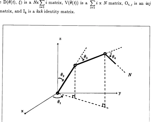
For an N dof manipulator as shown in Figure 1.2, using the

Denavit-Hartenberg matrix representation (Appendix A) for the manipulator linkage and

the Lagrange-Euler formulation as outlined in Appendix B, the dynamic equations

describing the motion of the manipulator in the absence of actuator dynamics,

friction, and other disturbances can be written in the following matrix form:

where

M(B(t), ~) 8(t)

+

D(B(t), 8(t),

e)

+

G(B(t),~) = T(t) ,

B(t)

=

[Bl(t), B₂(t), . .. , BN(t)]T B( t) E?RN , 8( t) E?RN , 8( t) E ?RN

(46)

11(8(t), ~)

D ( 8(

t),

8(

t),

~) G(8(t), ~)

T(t)

8(t), 8(t), 8(t)

NxN inertia matrix

Nx1 vector of Coriolis and centrifugal forces

Nx1 vector of gravitational forces

Nx1 vector of generalized driving forces/torques applied

by the actuators at the drive points on each link of the manipulator

Nx1 vectors of generalized joint displacements, velocities,

and accelerations respectively

a vector (with appropriate dimension) of parameters of

the mechanism such as payload, which belong to the

finite region of allowable parameter values

:=,

that is, ~

E

:=.

In general, the elements of the 11(8(t), ~), D(8(t), 8(t), ~), and G(8(t), ~)

matrices are functions of the dynamic parameters of the manipulator (lengths,

masses, load, etc.) as well as the instantaneous configuration (position) of the

links, while the elements of the D( 8(

t),

8(

t),

~) matrix also depend on the instantaneous velocity of the links. Thus, the elements of these matrices are

strongly varying while the manipulator is in motion.

The inertia matrix 11( 8( t), ~) is positive definite, bounded, symmetric and

always invertible for all 8(

t),

~, and

t

[Balestrino et.al, 1983; Paul, 1981; Tourasis

and Newman, 1985]. The inertia and the gravitational terms are particularly

important in manipulator control as they affect the system stability and positional

accuracy of the manipulator. It is generally assumed that the Coriolis and centrifugal forces are significant only when the manipulator is moving at high

speed. At low speed, their effects are small [Paul, 1981; Tourasis and Newman,

1985].

The Coriolis and centrifugal vector D( 8(

t),

8(

t),

~) can also be written in the following form [Lim and Eslami, 1985] :

(47)

o

N-I,l iJ_{2 (}

t)

I_{N _I}

V(iJ(t)) (1.3)

_ N

N

where D(O(t), ~) is a Nx ~ i matrix, V(iJ(t)) is a _~_i_x _N_matrix,_Oi,j_{is an}_ixj i=l

i=l

null matrix, and Ik is a kxk identity matrix.

z

,

....

N

~~--~---~----+y

~

... tl

I

8 ... ... I

1 ...

ll

..

x

FIGURE 1.2 N dof Robot Manipulator

[image:47.671.110.598.319.713.2]

(48)

multi-output system, described by a set of coupled, nonlinear time varymg

second-order differential equations, resulting from the dynamic interactions among

the links of the manipulator arm. However, in designing the controller for a robot

manipulator, the majority of current industrial approaches ignore the coupled,

time varying dynamic equations and treat the robot manipulator as a set of

simple, decoupled, linear time invariant servomechanisms. However, the changes

in the parameters of the controlled system due to the nonlinear time varying

dynamics are significant enough to render the linear servomechanism strategy

ineffective for fast and high-precision tasks [Fu et.al., 1987; Spong and Vidyasagar,

1989].

In contrast to the current industrial approaches where the controller is

normally designed based only on the actuators dynamics, the advanced control

strategies proposed in much of the literature on robot manipulator control, were

designed based only on the dynamic model of the mechanical part of the robot

manipulator (equation 1.1); the dynamics of the actuators which are part of the

whole robot manipulator system have generally been ignored, and the drive

torques or forces are modeled as pure torque/force sources or as first order lags

[Good, 1985]. This, in the majority of cases, is a simplification of a much more

realistic model of the system [Ailon, 1988].

1.3 MANIPULATOR CONTROL STRATEGIES

The robot manipulator control system is basically organized in a vertical

hierarchical fashion which consists of several control levels. The question of how

many different levels should there be in the hierarchical structure is dependent on

the type of the robot manipulator and the complexity of the tasks for which the

robot manipulator is intended. One thing certain is that all robot manipulators

have the lowest two control levels, namely, the tactical level which generates the

desired trajectories of each dof of the manipulators, and the executive level which

executes these trajectories by producing proper drive signals, through a suitable

control algorithm, to the appropriate actuators incorporated in each dof of the

(49)

subdivided in a number of separate hierarchical levels [Vukobratovic and Stokic,

1982].

Ideally, the aim of robot manipulator controller at the executive level is to

maintain a prescribed motion for the manipulator along a desired trajectory

generated at the tactical level, and in accordance with some prespecified system

performance. The majority of current industrial approaches to the robot arm

control design treat each joint of the manipulator as a simple linear

servomechanism with, for example, proportional plus derivative (PD), or

proportional plus integral plus derivative (PID) controllers. In designing the

controllers, the nonlinear, coupled and time-varying dynamics of the mechanical

part of the robot manipulator system have usually been completely ignored, or

assumed as disturbances. They generally give satisfactory performance when

properly tuned and driving only one joint at a time. However, when the links are

moving simultaneously and at high speed, the nonlinear coupling effects and the

interaction forces between the manipulator links may decrease the performance of

the overall system and increase the tracking error. The disturbances and

uncertainties such as variable payload in a task cycle may also reduce the tracking

quality of the robot manipulator system [Vukobratovic et.al., 1985]. Thus, the

method is only suitable for relatively slow manipulator motion and

limited-precision tasks [Craig, 1986; Fu et.al. 1987; Spong and Vidyasagar, 1989].

In the past years, various advanced and sophisticated control strategies at

the executive level of the control hierarchy have been proposed by numerous

researchers for controlling the robot manipulator such that the system is stable as

well as the motion of the manipulator arm is maintained along the prescribed

path generated by the tactical level. The structures of these controllers can be

loosely grouped into three categories, namely, the centralized, decentralized, and

multilevel hierarchical structures. In the following, some of these control

approaches which have been reported in the literature will be briefly presented.

A number of centralized control schemes have been developed for

improving the control of the nonlinear, coupled time varying robot manipulator.

These include among others, the Computed Torque techniques [Markiewicz, 1973;

Bejczy, 1974; Craig, 1986] or the Inverse Problem methods [Raibert and Horn,

(50)

et.al., 1980a; Wu and Paul, 1982], the Nonlinear Decoupled Control methods

[Freund, 1982; Kuo and Wang, 1989], the Variable Structure Control approaches

[Young, 1978; Slotine and Sastry, 1983; Chen et.al., 1990; Fu and Liao, 1990;

Wijesoma and Richards, 1990; Song and Gao, 1991], the Self-Tuning Control

methods [Koivo and Guo, 1983; Leininger, 1984], and the Model Reference

Adaptive Control strategies [Dubowsky and DesForges, 1979; Balestrino et.al.,

1983; Osman, 1985; Tzafestas and Stavrakakis, 1986; Chen, 1987b; Ambrosino

et.al., 1988].

The Computed Torque Technique [Markiewicz, 1973; Bejczy, 1974; Craig,

1986], also called the Inverse Problem method [Raibert and Horn, 1978; Paul,

1981], is basically composed of a feedforward and a feedback component. The

methods require exact modeling of the manipulator arm dynamics. Based on the

manipulator dynamic model and the desired joint trajectory, the feedforward

component computes the required input torques to compensate the actual

manipulator arm dynamics such that the nonlinear coupled manipulator system is

reduced into a linear decoupled time invariant system. Then, based on a standard

linear control technique, the feedback component is designed to control the linear

decoupled system. One of the main drawbacks of these control methods

[Markiewicz, 1973; Bejczy, 1974; Paul, 1981; Craig, 1986] is that they require

on-line computation of the joint torques based on the complete Lagrange-Euler

dynamic equation of the robot manipulator, which is very inefficient. Raibert and

Horn [1978] used a partial table look-up approach to simplify the computation

automatically in the control computer rather that to compute the nonlinear

dynamic equations. The disadvantage of this scheme is that it requires a large

computer memory. Another problem with these methods is that their validity is

questionable when there is a significant difference between the computed torque

model parameters and the actual robot manipulator parameters.

Resolved motion means that the motion of the various joints are combined

and resolved into separately controllable end-effector motion along the task

coordinates axes (Cartesian coordinate system) [Fu et.al, 1987]. The Resolved

~10tion Control strategies include the Resolved ~fotion Rate Control ['Vhitney,

1972], Resolved ~10tion Acceleration Control [Luh et.al., 1980a], and Resolved

Motion Force Control [Wu and Paul, 1982]. In Resolved ~10tion Rate Control

(51)

time varyIng speeds along the axes relevant to the task coordinate in order to

achieve desired coordinated end-effector motion. The method requires the

computation of the inverse of the Jacobian matrix at each sampling time for the

calculation of the joint rate (velocity). The disadvantages of this method are that

the inverse Jacobian matrix requires intensive computations, and matrix inversion

may cause singularity problems. The Resolved Motion Acceleration Control

method [Luh et.al., 1980a] is simply an extension of the Resolved Motion Rate

Control technique, which includes acceleration control. It assumes that the desired positions, velocities and accelerations are available. The method is quite

similar to the Computed Torque Technique except that the desired trajectory and

the feedback law are expressed in terms of the task coordinates. This control

technique has the same disadvantages as the Revolved Motion Rate Control

technique and the Computed Torque technique. Resolved Motion Force Control

[Wu and Paul, 1982] is based on the relationship between the forces obtained from

wrist force sensors and the joint torques at the joint actuators. The controller

consists of the Cartesian position control which calculates the desired forces to be

applied to the end-effector in order to track the desired task trajectory, and a

force convergent control which determines the required joint torques to be applied

to each joint actuator such that the end-effector has the desired forces applied as

determined by the Cartesian position control. The method avoids the

computation of the inverse Jacobian matrix and complicated dynamics of the

robot manipulator. However, the convergent rate of the force convergent control

depends on the structure of the manipulator, and the calculation of the dynamic

model is replaced by an iterative stochastic method which also demands extensive

computation [Vukobratovic et.al., 1985].

A nonlinear feedback pole placement control method for controlling a robot

manipulator was proposed by Freund [1982]. The control algorithm consists of

two parts. The first part is the nonlinear decoupling control which completely

decouples the nonlinear robot manipulator dynamics into a set of decoupled linear

input-output second order differential equations whose characteristic coefficients

can be chosen arbitrarily. The second component of the Nonlinear Control

Algorithm is an arbitrary pole placement technique to design the dynamics of the

linear input-output second order equations, obtained from the first part, as

Decentralized and hierarchical control of robot manipulators

City, University of London Institutional Repository

DECENTRALIZED AND HIERARCHICAL CONTROL

OF ROBOT MANIPULATORS

TABLE OF CONTENTS

8,

°

Q.

,

Q.

LIST OF TABLES

LIST OF FIGURES

=

=

=

=

=

=

=

=

=

Q.

Q.

Q.

Q.

=

=

=

=

=

=

=

=

=

=

=

ACKNOWLEDGEMENTS

DECLARATION

PUBLICATION

ABSTRACT

A(

LIST OF SYMBOLS

OJ,

OJ,

OJ,

B( .,.,.)

B

8

B

B

C(

C ..

D ..

ili,

L

D(

G(

0i,

0

o

9G(.,.)

T

T(.)

=

T

T(

=

v··

L

OJ,

OJ

OJ,

OJ

OJ

OJ

Xp(

X

t)

t)

t)

_,

_•

_,

,,*)

,,*)

,)