Robust Hybrid Motion Force Control Algorithm for Robot Manipulators

ROBUST HYBRID MOTION-FORCE CONTROL

ALGORITHM FOR ROBOT MANIPULATORS

V. A. Mut, J. F. Postigo, R. O. Carelli and B. Kuchen

Instituto de Automatica, Universidad Nacional de San Juan San Juan, Argentina, [email protected]

(Received: October 3, 1998 - Accepted: June 3, 1999)

In this paper we present a robu st hybrid motion/force controller for rigid robot

Abstract

manipulators. The main contribution of this paper is that the proposed hybrid control system is able to accomplish motion objectives in free directions and force objectives in constrained directions under parametric uncertainty both in robot dynamics and stiffness constraint constant. Also, the given scheme is proved globally stable in the sense that the control objectives are achieved asymptotically, when a signum function is used in the control law, though giving rise to chattering effects. To avoid this problem a saturation function is used. In this case the motion and force errors are proved to be bounded functions. U sing the proposed control stru cture there is no need to measure the derivative of the interaction forces. Some simulation results are given to illustrate the control system performance.

R obot Manipulators, Nonlinear Systems, H ybrid Motion-Force Control, R obust

Key Words

Control

» oíÇ« S Çw RBÇM°n ºBµn±U¿±P¼¯BÇ« nj °o¼Ç¯-S oe zi ³¯B£°j ¶k®® ¤oT® ð½ ³§B « ½A nj

²k¼ña

° jApC RB´] nj S oe AkµA k¯A±U»« ºjB´®z¼Q ³¯B£°j ¤oT® ©Tv¼w ³ SwA ½A ³§B « ½A ¶kªî ©´w /j±{»« An ²k{ j°kd« » { SMBY nAk « nj ©µ RBM°n ºB´ñ¼«B®½j nj ©µ ºoT«AnBQ ê «B¯ ½Ao{ nj kؼ « RB´] nj °o¼¯ AkµA j°n nB ³M ¤oT® éMBU nj ¨±®¢¼w éMBU ð½ ³ »«B¢®µ SwA ²k{ SMBY ³ B\¯C pA ¼®`ªµ /jpBw ²jn°C oM éMBU ð½ pA ³¦Ãv« ½A pA ºo¼£±¦] ºAoM /j±{»« nAk½BQ  ©Tv¼w k¯A²k{ ¥æBe K¯B\« S§Be ³M ¬k¼wn BM ¤oT® @ BM /k¯±{»« ¥½kLU nAk¯Ao éMA±U ³M °o¼¯ ° S oe ºBµB i S§Be ½A nj ³ j±{»« SMBY /j±{»« ²jB TwA BL{A ©Tv¼w jo nB y½Bª¯ ºAoM /Sv¼¯ yz ©µoM ºBµ°o¼¯ Tz« ºo¼£@²pAk¯A ³M ºpB¼¯ ,¤oT® nBTiBw ½A pA ²jB TwA /SwA ²k{ ³ÄAnA ºpBw ³¼L{ jn±« k®a [½BT¯ ¤oT® @

INTRODUCTION

C o n t r o l o f r o bo t ic m a n ip u la t o r s ca n be classified into two different approaches: motion control and constrained motion control. Motion Control is used when the robot arm moves in a fr e e sp a ce wit h o u t in t e r a ct in g wit h t h e environment. Motion control specifications are given in te rms of a desired mot ion trajectory. O n t h e o t h e r h a n d, C o n st r a in e d M o t io n Control of robots is concerned with the control o f r o b o t s wh o se e n d -e ffe ct o r in t e r a ct s mechanically with the environment, which leads to control schemes that regulate the interaction

fo r ce s be t we e n t h e e n d-e ffe ct o r a n d t h e environment [1]. Most assembly operations and ma n u fa ct u r in g t a sk s r e qu ir e m e ch a n ica l interactions with the environment or with the o bje ct be in g ma nipu la t e d, a lo ng wit h fa st motion in free and unconstrained space. Several controller schemes have been proposed in the lit e rat ure and can basically be classifie d as compliant motion control, pure force control, and hybrid motion-force control [2,3].

cance llation of the nonlinear dynamics. The uncert ainty in some robot parameters, as link ine t ria and payload, normally de grade s the control performance. In this context, there exist two basic approaches to reduce the effe cts of uncertainties: adaptive robot control and robust robot control [15,16]. Adaptive controllers for motion and const raine d motion robots have be e n pr o po se d in t h e lit e r at u re [4,5,6,7]. R egarding the robust control approach, there e xist so me sch e me s wit h glo ba l st a bilit y de monstrat ions to solve t he motion control problem [8,9], and a robust adaptive motion -force controller [10].

In this pape r, we pre se nt a robust hybrid motion-force controller for robot manipulators as an extension of the robust motion controller in [9], using t he hybrid cont rolle r st ruct ure described in a previous work [7]. The controller has a simple structure as a result of being based upon robot model parameterization and the use of switching functions. The controller is robust t o u n ce r t a in t ie s bo t h in t h e ma n ip ula t o r dynamics and the environme nt stiffness. This approach does not require measurement of the joint acce le rat ion or t he force derivative. A global stability demonstration is given based on Lyapunov analysis, wit hout any linearization assumptions. Also, bounde dne ss of control errors is proved when a sat uration function is used to avoid chattering.

The paper is organized as follows. In section I I we summa r ize th e ma n ip ula t o r mode l. Section III presents the problem formulation. The proposed robust hybrid controller is given in section IV. In sect ion V we de scribe some simulation results, and finally in section VI the concluding remarks are given.

ROBOT MODEL

I n t h e a b se n ce o f fr ic t i o n a n d o t h e r disturbances, the Cartesian-space dynamics of

an n-link constrained rigid robot manipulator can be written as,

. . ..

(2.1) H(x)x + C(x,x)x + G(x) + F = J-T

t

where x is the nxl vector of Cartesian position a n d E u l e r a n gle s o f t h e m a n i p u l a t o r end-effector, in a reference frame R₀fixed to the robot base;

t

is the nxl vector of torques (or for ce s) ap plie d t o t h e r obot jo in t s by th e actuat ors; H ( x) is the nxn symme tric positive

. . definite manipulator inertia matrix, C(x,x)x is the nxl vector of centripetal and Coriolis forces, G ( x) is t he nxl vect or of gravitat ional force s; J( q) is t he nxn manipulator J acobian mat rix, assumed to be nonsingular, q is the nxl vector of joint displaceme nts and F is the nxl vect or of interaction force/moments at the end-effector. In case J be singular due to arm singularities or J be non-square due to arm re dundancy, it is necessary to apply the generalized inverse based on the singular value decomposition theorem, so that the null space existing in Cartesian space o r j o i n t sp a ce ca n b e se p a r a t e d . T h e man ipu lat or de scr ibe d by E qu at ion 2.1 is assumed non-redundant. It is assumed that the r obot is e qu ip p e d wit h join t p osit ion an d ve lo cit y se n sor s a n d a for ce se nso r a t it s end-effector. Although the motion Equation 2.1 is co m p le x, it h a s se ve r a l fu n d a m e n t a l p ro pe r t ie s which ca n be u se d t o e ase t h e control system. The properties are as follows:

(See[4]). By using a proper definition

Property 1

. . .

of matrix C( x,x) ( only t he ve ct or C( x,x)x is . uniquely defined), matrices H (x) and C(x,x) in Equation 2.1 satisfy

.

"

z

û

Rn ZT [dH(x)/dt - 2C(x,x)] z = O

( Se e [4]). A pa rt of t he dynamic

Property 2

st ruct ure 2.1 is line ar in t e rms of a suit able selected set of robot and load parametes, i.e.

. .. . .

..

. ..

Where

W

(x,x,x) is an nxm matrix and

q

is an mxl ve ct o r co n t a in in g t h e r o b o t a n d lo a d parameters.

(See [6]). H(x) is an nxn symmetric

Property 3

positive definite matrix and there is a constant

a>

0 such that

"

x

û

Rn

a

I

À

H(x)

For revolute joint robots if, in addition, J-1(q) is a b o u n d e d n xn m a t r ix, t h e n t h e r e is a

b

(

a<b<È

) such that,

a

I

À

H(x)

À b

I

"

x

û

Rn

PROBLEM FORMULATION

Following Raibert and Craig [3] and Slotine and Li [4] two coordinate systems are defined. The first one-already defined in section II- is a frame of reference R₀ fixed on the robot base, which de fine s a Carte sian space called ope rational sp a ce . I n t h is sp a ce , t h e e n d -e ffe c t o r configuration is represented by using a vector x, composed of the Cartesian position and E uler angle s of the end-effector. The se cond is the compliance frame R_c( also calle d const raint frame), which is used to describe the compliant motion t ask. It is nat urally defined by the so ca lle d n a t u r a l co n st r a in t s, so t h a t t h e coordinates be associated to the unconstrained and the constrained directions in the task space. Without loss of generality, we assume that both coordinate frame s R₀and R_ch ave t he same o r igin . I n ge n e r a l, t h e R_c fr a me ma y be time-varying. Task spe cificat ions can now be give n in t h e co m p lia n ce fr a m e : m o t io n specifications in the free directions and force specifications in the constrained directions.

We digress mome ntarily to establish some . .. nomenclature used henceforth. Vectors x, x, x ar e re spe ct ive ly t h e posit ion, ve locity a nd acceleration of the end-effector specified in the frame R₀. F is the interaction force between the

environment and the end-effector specified in the same frame R₀. Note that he re "position" me a ns bot h p osit io n an d o rie n t a t ion , an d "force" implies bot h force and torque. In t he compliance frame R_c, position, ve locit y and

. ..

a cce le r a t io n a r e e xp r e sse d by x_c , x_c , x_c respectively and force by F_c. Position and force refe rence t raje ctories spe cified in t he same_{. ..}

. ..

frame are given by x_cd, x_cd, x_cd, F_cd, F_cd, F_cd. The fort hcoming analysis nee ds a transformation mat rix R

û

Rn xn be t we e n complia nce an d operational coordinates. This matrix, a rotation matrix, is defined by the interaction task surface and is given by t he task planne r. In ge neral

. R = R ( t ) is t im e -va r yin g, R a n d R a r e a ssume d bou nde d a nd R h as it s minimu m singular value bounde d away from zero (t hus i m p l yi n g t h a t R- 1 = RT i s b o u n d e d ) .

.. .

Be side s, RT and RT e xist an d ar e assume d bounded, too. Conditions on the derivatives are n at u rally sat isfied fo r smoot h t ask surfaces. Therefore, the following relations hold:

x_c= RT(t)x

. _.

.

x_c= RT(t)x + RT(t)x .

.. _{. ..}

.. _(3.1)

x_c= RT(t)x + 2RT(t)x + RT(t)x F_c= RT(t)F

. .

.

F_c= RT(t)F + RT(t)F

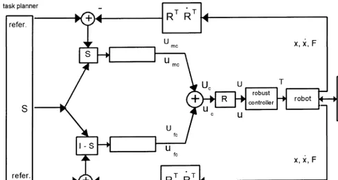
Figure 1. Control structure.

The manipulator is assumed to be equipped with a force sensor at its end-effector. Now it is nece ssary t o conside r t he inte raction mode l wh ic h ge n e r a t e s r e a c t i o n f o r ce s. T h e environment is modelled by a stiffness matrix K_e as,

(3.2) F_c = K_e [x - x_e]_c = K_e [x_c - x_ec]

with x_ec(t) the position of the constraint point which is current ly int eract ing wit h t he e nd -e ff-e ct or . In t his pap-e r w-e con sid-e r a st at ic

.

environment, so x_{e c}= 0. K_eis assume d to be uncert ain but const ant . Like wise , we could also consider a rigid environment, for instance, t he part s asse mbly and polish applicat ions. H ere, a compliance model with stiffness matrix is then associated with the force sensor.

We are now ready t o formulat e t he robust motion/force control problem. Let us consider the manipulator described by Equation 2.1. The parameter vector

q

-from properties of [4]- of the manipulator, payload and environment is constant but unknown. The robot Jacobian

matrix J(q) is assumed to be non-singular and known. Knowledge of J ( q) is not re st rict ive because it does not de pend on the dynamic paramete rs. The hybrid motion/force cont rol specificat ions are given in t erms of a de sired mot ion trajectory x_cd( t) in the unconstrained directions and a desired force trajectory F_cd(t) in the constrained directions.

The robust hybrid control proble m can be st at e d as t hat of de signing a cont rol law t o compute the joint applied torques

t

, so that the following objectives be verified:

a) S(x_cd(t) - x_c(t))

Ø

0 as t

Ø È

in the unconstrained directions, and b) S'(F_cd(t) - F_c(t))

Ø

0 as t

Ø È

in the constrained directions.

ROBUST HYBRID CONTROLLER

Let us consider the control

Robust Controller.

coordinates of the compliance frame R_c, and t h e o t h e r f o r co n t r o llin g f o r ce in t h e constrained coordinates.

A mot ion/force cont rolle r base d o n t he structure given in [7] with estimated values of the robot dynamic model is,

. .

.. _.

J-T

t

= H₀[u - RRTx - 2RRTx - RRTv] +

. _(4.1)

C₀[x-

n

] + G₀ + F

whe re H₀, C₀, G₀ have t he same functional forms as H(x), C (x) and G(x) respectively, with e st imat e d dyn amic para me t e rs. The sign al vectors u and v are related to the corresponding vectors expressed in the compliance frame R_c by the transformation R as,

(4.2) u = R(t) u_c ;

n

= R(t)

n

_c

where u_cand

n

_care obtained from the motion and force control loop components (see Figure 1) as,

(4.3) u_c= u_mc + u_fc ;

n

_c =

n

_mc +

n

_fc.

where

n

_mc and

n

_fc , u_mc and u_fcare orthogonal, respectively.

Vectors u_mc,

n

_mc are defined as, .

-1 ..

(4.4)

n

_mc = x_cd + M_m [B_me_xc+ K_me_xc] . ..

-1

n

_mc = -[l/(

r

+

l

)] M_m [M_me_xc+ B_me_xc+ (4.5) K_me_xc]

Likewise, vectors u_fc,

n

_fc are calculated as, .

..

(4.6) u_fc = S'K_e-1[F_cd + M_f-1 (B_fe_fc + K_f e_fc)]

. ..

n

_fc= -[l/(

r

+

l

)] S'K_e-1M_f-1[M_fe_fc+ B_fe_fc+ (4.7) K_fe_fc]

In E qu at io n s 4.3-4.7, exc = S(xcd - xc ) and

efc = S' ( Fcd - Fc ) are the posit ion and force erro rs respectively expr essed in t he complian ce frame. Also, S' = In - S,

r

=d(.)/dt,

l

is a positive design scalar and Mm , Bm , Km , Mf, Bf, Kfn are n xn p o sit ive d e fin it e a n d d i a go n a l d e sign

. .

matrice s. Note t hat xc , xc , F. c , Fc are o bt ain e d from measured values of q , q and F by using the r e la t io n x = f( q ) be t we e n x a n d q , a n d Equations 3.1 and 3.2.

Vect ors

n

_mc and

n

_fc in E quat ions

Remark 1.

4.5 and 4.7 can be written as,

. .

n

_mc = -[

r

/(

r

+

l

] e_xc- [l/(

r

+

l

)] M-1_m (B_me_xc + K_me_xc)

.

n

_fc = - [

r

/(

r

+

l

)]S'K_e- 1e_fc-[l/(

r

+

l

)]S'K_e-1 .

(4.8) M_e-1 (B_fe_fc + K_fe_fc)

The above e xpre ssions and E quat ion 4.1 clearly show that the computation of

t

requires

k n o w l e d g e

.

of end-effector posit ion x, velocity x, force F and .

i t s d e r i va t i ve F ( n o m e a s u r e m e n t o f

a c c e l e r a t i o n

.. ..

x and second derivative of force F is required).

. .

T o a vo id m e a su r i n g F , F_c in

Remark 2.

Equations 4.6 and 4.8 can be computed as .

. .

(4.9) F_c= K_e(x_c - x_ec).

Ve ct ors

n

_{m c} a nd

n

_{m c} de fin e d in

Remark 3.

E qu a t io n s 4.4 a n d 4.5 h a ve co mp o n e n t s corresponding only to the unconstrained task space coordinat e s and vect ors u_fc and

n

_fcin Equations 4.6 and 4.7 have components only in the constrained coordinates. This comes from using sele ction matrice s S and S' which select t h e comp o n e nt s o f t h e mot io n a n d fo r ce controlled directions respectively. Consequently, u_mc, u_fcas well as

n

_mc,

n

_fc represent a partition of u_cand v_crespectively in Equation 4.3.

Now, considering E quation 4.6 and R emark 2, we can write

. . ..

u_fc= S'K-1_eF_cd+ S'K-1_e M-1_fB_fS'K_e (x_cd- x_c) + S'K_e-1M-1_fK_fe_fc

. . ..

(4.10) u_fc= K_elF_cd+ K_e2(x_cd - x_c) + K_e3e_fc

where

K_e1 = S'K_e-1

K_e2 = S'K_e-1 M_f-1B_f S'K_e K_e3 = S'K_e-1 M_f-1K_f

Likewise, considering E quation 4.7, R emark 1 and Remark 2 yield,

..

.

M_f-1(B_fe_fc + K_fe_fc)

. .

.

n

_fc= [

r

/(

r

+

l

)] S'K_e-1S'K_e(x_cd- x_c) - [

r

/(

r

+

l

)]

S' K_e-1 M_f-1 B_f e_fc

- [l/(

r

+

l

)] S' K_e-1 M_f-1K_f e_fc . .

v_fc= -[

r

/(

r

+

l

)]K_e4 (x_cd- x_c)

-(4.11) [

r

/(

r

+

l

)]K_e5e_fc- [l/(

r

+

l

)]K_e6e_fc

where:

K_e4 = S'K_e-1S'K_e K_e5 = S'K_e-1M_f-1B_f K_e6 = S'K_e-1M_f-1K_f

Now, base d on control law E quation 4.1, properties of [4] and E quations 4.10 and 4.11 with parame te rization of u and v signals in t e r m s o f K_e, we p r o p o se t h e fo llo win g

motion/force control law _{. ..}

.. . .

J-T

t

=

f

(x, x, x_cd, x_cd, x_cd, F , F_cd, F_cd, F_cd, R , ..

.

(4.12) RT,RT)

q

₀ + F

where

f û

Rnxm is a signal matrix and

q

₀

û

Rm is the uncertain robot and stiffness parameters ve ct o r. In E quat ion 4.12,

t

r e pr e se nt s t he control actions, i.e . t he torques/forces t o be applied to the robot joints.

Now, based on control law Equation 4.12, we propose t he following robust motion /force control law, . .. . . .. .

J-T

t

=

f

(x,x,x_cd,x_cd,x_cd,F,F_cd,F_cd,F_cd,R , RT , ..

(4.13) RT)

q

₀-

f

(.) K sign(

f

T(.)

n

) + F

where K is a constant nxm matrix to be defined in IV.3. This control law has a similar structure to that of [9] for pure motion robot control.

Before carrying out the stability

Error Model

analysis, it is necessary to obtain the so called error model [11], which relates dynamically the signal vector v and the parameter error vector

¬

q

=

q

₀ -

q

. B y e qu a t in g r o bo t mo d e l o f

E q u a t i o n

2.1 an d t he con tr ol la w of E qua tion 4.13, we obtain_{.. .}

H x + CX + G + F =

fq

₀ -

f

K sign(

f

T

n

) (4.14) + F

. _¬

Now, by substituting

q

₀=

q

+

q

into Equation 4.14 and observing from Equations 4.12 and 4.1 that,

. . .

. ..

fq

= H[u-RR T x-2RRT x-R

n

_c] + C[x -

n

] + G the closed loop Equation 4.14 results

.

.. _¬

H(x-u') + HR

n

_c+ C

n

=

f q

-

f

K

(4.15) sign(

f

T

n

)

with

.

.. _.

u' = u - RRTx- 2RRTx. ..

The evaluation of (x-u') now follows, ..

..

(x - u') = RRT (x - u') where . . .. .. ..

RT (x-u') = RT x - RT u + RT x + 2RT x. But, from Equations 3.1 and 4.2,

.. ..

RT(x - u') = x_c- u_c.

Now consider the following partitions in free and constrained directions

.. .. ..

x_c= x_mc + x_fc ; u_c= u_mc + u_fc with

.. ..

.. ..

x_mc = Sx_c ; x_fc= S'x_c. Then,

.. ..

.. ..

RT(x - u') = x_c- u_c = (x_mc - u_mc) + (x_fc -(4.16) u_fc).

Manipulating E quations 4.4 - 4.5, 4.6 - 4.7 and the stiffness model of Equation 3.3, yields

. ..

. ..

x_mc - u_mc =

n

_mc +

ln

_mc ; x_fc- u_fc=

n

_fc+

ln

_fc

Then, Equation 4.16 can be written as .

. ..

RT(x - u') = (

n

_mc +

n

_fc) +

l

(

n

_mc +

n

_fc)

and considering vector partition of Equation 4.3 .

..

RT(x - u') =

n

_c +

ln

_c.

Now, from Equation 4.2 and

. .

.

n

= R(t)

n

_c ;

n

= R(t)

n

_c + R(t)

n

_c

(x-u')=RR T(x-u')=R(

n

_c+

ln

_c) =

n

+

l n

-R

n

_c. Going back to Equation 4.15, we obtain

(4.17) H(

n

+

ln

) + C

n

=

fq

-

f

K sign (

f

T

n

)

E quation 4.17 describe s t he so calle d e rror model equation.

N o w we s t a t e t h e m a i n

Main Results

properties of the proposed robust controller in the following proposition.

Proposition 1. Conside ring the control law E q u a t io n 4.13 in clo se d lo o p wit h t h e manipulator Equation 2.1, the following holds,

n n

a)

n û

L₂

ú

LÈ n n

b)

n

_mc,

n

_fc

û

L₂

ú

LÈ n n

.

c) e_xc, e_xc

û

L₂

ú

L_È, e_xc

Ø

0 as t

Ø È

n n

.

êêê

d) e_fc, e_fc

û

L₂

ú

LÈ , e_fc

Ø

0 as t

ØÈ

.

We note that c) and d) in proposition 1 ensure that the control objectives of Equations 3.4 and 3.5 are verified.

Proof. Consider the error model of Equation 4.17, and the following non negative function of time (remember property 3),

(4.18) V(t) = 1/2[

n

T H

n

]

whose time derivative along the trajectories of Equation 4.17 is,

.

V = -

ln

T H

n

+

n

T

f q

-

n

T

f

K sign (

f

T

n

) (4.19) Where we have used the property 1 to eliminate the term

n

T (1/2H-c)

n

.

. ¬

Taking K = diag (k_i) with K_i

 ´q

_i

´

, then V in E qua t ion 4.19 sa t isfie s V ( t )

Â

0. T his

n

implies that

n û

L_È. Also H is lower bounded as established by property 3. Then integrating Equation 4.19 from 0 to T and considering T in

n

the limit, it verifies that

n û

L₂. This establishes a).

Now, from E quation 4.3 and R emark 3, we can write the following vector partition,

RT(t)

n

=

n

_c =

n

_mc +

n

_fc

a n d r e ca llin g t h a t R wa s a ssu me d t o be

bounded, from a) we immediately conclude b).

n n

F in a lly, a s

n

_{m c},

n

_{f c}

û

L₂

ú

L_È , fr o m Equations 4.5, 4.7 and lemma shown in Desoer and Vidyasagar (1975), pp. 59 [13], we derive c)

êêê

and d).

The control law of E quation 4.1

Remark 4

cont ains the signum funct ion. As a result we might expect ``chattering'' to occur. In order to alle viat e t his sit uation, we ca n re place the sign um fu n ct ion by t h e mxl ve ct o r o f t h e saturation function sath= (sat(₁), ..., sat(h_i), ..., sat(h_m))T, defined as,

hi

>1

æ

1

(4.20) -1<hi<1

sat(h_i)

Û å

hi<-1

¦

-1

where h_iare the components of the mxl vector h=

f

T

n

/

e

, wit h i= 1, ..., m and

e

> O , a nd h_i con t a in in g t h e bo un ds for t he commu t ing switching planes [12]. By using the saturation function, the convergence of the control errors can not be concluded towards zero but to their bounds.

Proposition 2. Consider the control law .. . ..

. .

J-T

t

=

f

(x,x,x_cd,x_cd,x_cd,F,F_cd,F_cd,F_cd, ..

.

(4.21) R,RT,RT)

q

₀-

f

(.) K sat[(

f

T(.)

n

)/

e

] + F

where sat(.) is defined in E quation 4.20. Then, the control errors are ultimately bounded. Proof. Consider t he error model of E quat ion 4.17, where sign(.) is substituted by sat(.), and t he fo llo win g n on n e ga t ive t ime fu nct io n (remember property 3),

.

(4.22) V(t) = 1/2[

n

TH

n

]

whose time derivative along the trajectories of the error equation is

~

.

V = -

l n

T H

n

=

n

T

f q

-

n

T

f

K sat( ____)

f

T

n

e

(4.23) When sat(h_i) = h_iwe can rewirte Equation 4.23 as

~

.

(4.24) V = -

a

V +

n

T

f

(

q

+ u)

By inspecting the second term of Equation 4.24

~

and recalling K= diag( K_i) wit h K_i

 ¼q

_i

¼

, it follows

~

n

T

f

[

q

+ u]

À n

T

f

[K sign(

f

T

n

) - _______] =K

f

n

T

T

n

e

(4.25)

f

K [sign(

f

T

n

) - ______]

f

T

n

e

~

n

T

f

[

q

+ u]

À n

T

f

[K sign(

f

T

n

) - _______]K

f

À

T

n

e

´n

T

f´ l

_max(K)[

¡

(m) - ___________]

´

(

f

T

n

)

´

e

The funct ion de fine d in E quation 4.25 has a maximum for:

´f

T

n´

= (

¡

m __)

e

2 Whose value is

(4.26) [m

l

_max(K) __].

e

4

By subst it uting E quat ion 4.26 int o E quation 4.24 we obtain

.

(4.27) V

À

-

a

V +

r

where

r

= [m

l

_max(K)__].

e

4

Considering E quation 4.27 it is clear that, V(t) (4.28) is ultimately bounded by

r

/

a

.

From Equation 4.22 it holds

(4.29) V

Â

__1

g

(H)

´

v

´

2

2

where

g

(H) = inf_q(

l

_min(H)).

From E quations 4.27 and 4.28 we conclude that

´

v

´

2 is ultimately bounded by 2

r

/

ag

(H). R eme mbering t hat v= R v_mc+ R v_fc, then the bounds of v_mcand v_fcare established from the bounds on v. Now, considering the

´

.

´

Èof the

filtering operators given by E quations 4.5 and 4.7, we obtain the bounds of motion and force errors, i.e.,

´

e_mc

´

È

À b

₁

´n

_mc

´

È

with

b

₁= _______ + ________4e -1

m_m-1b_m

l

m_m-1k_m .

´

e_mc

´

È

À b

₂

´

v_mc

´

È

with

b

₂= 1+ _______4

l

e-1 (4.30) m_m-1b_m

´

e_fc

´

È

À b

₃

´

K_e

n

_fc

´

È

with

b

₃= _____ + ______4e-1 m_f-1b_f

l

m_f-1 K_f

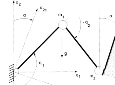
Figure 2. Two link manipulator and its environment.

For the case K_e = diag (k_e) is verified that

´

e_fc

´

È

À b

₃k_e

´n

_fc

´

È .

SIMULATION RESULTS

Computer simulations have been carried out to show the performance of the proposed robust con t r olle r. Th e ma n ip u lat o r u se d fo r t h e simulations is a two degree of freedom arm in a vertical plane, in contact with its environment as shown in Figure 2.

In this particular case R is a constant matrix given by,

sin

a í

æ

cos

a

¤

; with

a

= 0

Ü

.

R =

¤

cos

a ã

¦

-sin

a

Selection matrix is specified as S = diag [0, 1]. The manipulat or is mode le d as t wo rigid links of unitary length with masses m₁ and m₂ at the distal e nds of t he links. F rict ion is not considered in the model.

Sc a la r g i s t h e gr a vit y a c ce le r a t i o n magnitude. Numerical values of the parameters are m₁=4 kg, m₂=2 kg and K_e=1000 N/m. It is assume d t hat m₁, m₂, and K_e are uncertainly known.

From E quat ion 4.1, the vector cont rol law can be written as,

t

= JT

f q

₀+ JT

f

K sign (

f

Tv) + JTF =

fq

₀+ (5.1)

where the uncertain parameter vector, taken as

q

₀= [

q

₁₀

q

₂₀

q

₃₀

q

₄₀]T =

0.00125]T 1

0.00375 [3

is an estimation of:

q

= [m₁m₁/k_em₂m₂/k_e]T. We must note that in E quat ion 5.1,

f

= JT

f

, and K = diag [k₁, k₂, k₃, k₄].

M ot ion t ra je ct or y alo ng t he co nst r a in t surface is specified as,

x_cd(t)=(x _cd1,x_cd2)T= [0,0.5+0.2 cos(__t)]

p

T [m]

2

and force normal to the const raint surface is specified as

f_cd(t) = (f_cd1, f_cd2)T = [1 + 0.5 cos (__t),0]

p

T [N]

2

Simulation is carried out using the following design parameters (see Equations 4.5 and 4.7): M_m= diag [1], B_m= diag [10], K_m= diag [25], M_f= diag [1], B_f= diag [10], K_f= diag[250],

l

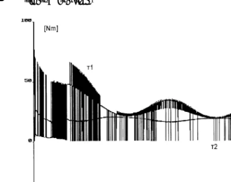
=30.

I n t h e fir st simu la t io n we co n side r t h e signum function in the control law. F igure 3 shows the e volut ion of force error e_fclin t he const raine d dire ct ion a nd t h e e volution of m o t io n e r r o r e_xc2 in t h e u n co n st r a in e d direction. For this case, torques

t

₁,

t

₂are shown in Figure 4. Note that motion and force errors converge to zero, but there is chattering in the torques applied to the joints.

In the second simulation, we conside r t he saturation function in the control law in order to avo id t he cha tte rin g pr oble m using t he signum function, which is observed in Figure 4. For this case, torques

t

₁,

t

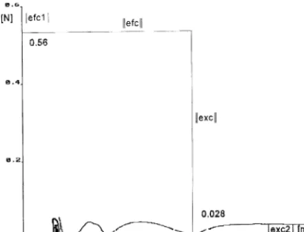
₂are shown in Figure 5. Note that the chattering effect is eliminated using the saturation function, but the mot ion an d for ce e rr ors do no t conve r ge t o ze r o, however they remain bounded. In Figure 6 we re pre se nt t he module of force e r ror in the constrained direction

§

e_fc1

§

versus the module of motion error in the unconstrained direction

§

e_xc2

§

. We observe in this last figure that this trajectory, according to E quations 4.30 and pp. 11 o f [14], r e ma ins u lt imat e ly bou nde d by

Fi gu r e 3 . F o r ce and m ot ion e r r or e volu t io ns u sing t he signum function.

Figure 4. Control actions (applied torques) when using the signum function.

Figure 6. Fo rce err or mod u le vs mo tion er ror mod u le when saturation function is used.

´

e_mc

´

È

Àb

₁

´n

_mc

´

È

Àb

₁

´n

_mc

´

₂ = 0.028 m

and by

´

e_fc

´

È

Àb

₃k_e

´n

_fc

´

È

Àb

₃k_e

´n

_fc

´

₂ = 0.56N.

CONCLUSIONS

In this pape r, a robust hybrid motion/force controller for rigid link manipulators has been pre sented. D ynamic parameters and stiffness con sta n t ar e a ssu me d t o be un kno wn bu t constant. The robust controller was shown to be globally stable in the sense t hat t he control obje ct ives are achie ved asymptotically when signum funct ion is used, occurring chatte ring effects. When we replace the signum function for a sat uration funct ion we avoid chat tering problems and bounded motion and force errors are verified. The controller is based on a hybrid mot ion/force st ruct ure , including nonlinear feedback of joint position and velocities as well a s t h e int e ra ct ive for ce . F o rce de r iva t ive m e a su r e m e n t is n o t n e ce ssa r y fo r t h is controlle r. Some simulation results for a t wo degree of freedom manipulator illustrate the controller performance.

ACKNOWLEDGMENT

This work was partially supported by CONICET - ARGENTINA.

REFERENCES

Spong M. W. and Vidyasagar M., "R obot D ynamics 1.

and Control", New York, John Wiley, (1989).

Whitney, D. E., "Historical Perspective and State of the 2.

Art in Robot Force Control", Int. J. Rob. Res., Vol. 6, (1987), 3-14.

R aibert M. H . and Craig J. J., "H ybrid Position/Force 3.

Control of Manipulators", ASME Trans. Dynam. Syst. J. Meas. Contr., Vol. 102, No. 2, (June 1981), 126-131. Slotine J. J. and Li W., "Adaptive Manipulator Control: 4.

A Case Stu dy",IEEE Trans. Automat.Contr., Vol. 33, No. 11, (Nov. 1988), 995-1003.

Kelly R. and Carelli R., "Unified Approach to Adaptive 5.

C o n t r o l o f R o b o t ic M a n ip u la t o r s", Proc. of the

IEEE-CDC, Austin, TX, USA, (Dec. 1988), 1598-1603.

Ortega R. and Spong M., "Adaptive Motion Control of 6.

Rigid Robots: A Tutorial", Automatica, Vol. 25, No. 6, (1989), 877-888.

C a r e lli R . a n d K e lly R ., "A d a p t ive H yb r id 7.

Impedance/Force Controller for R obot Manipulators", Proc. of the 11th IFAC World Congress, Tallin, Estonia, USSR, Vol. No. 9, (Aug. 1990), 274-279.

Abdallah C. et al., "Survey of Robust Control of Rigid 8.

Robots", IEEE Contr. Syst. Mag., Vol. 11, No. 2, (Feb. 1991), 24-30.

Sp o n g M ., "O n t h e R o b u st Co n t r o l o f R o b o t 9.

Manipu lators",IEEE Trans. Automat.Control, Vol. 37, No. 11, (Nov. 1992), 1782-1786.

Yao B. and Tomizu ka, M., "R obu st Adaptive Motion 10.

and Force Control of Robot Manipulators in Unknown Stiffness E nviro nments",Proc. of the IEEE-CDC, San Antonio, Texas, (Dec. 1993), 142-147.

An d e r so n B. D . O . e t a l., "St a b ilit y o f Ad a p t ive 11.

Systems: Passivity and Averaging Analysis", The MIT Press, Cambridge, MA, (1986).

H u n g J . Y ., G a o , W . a n d U n g, J . C., "V a r ia b le 12.

Stru ctu re Contr ol: A Su rvey",IEEE Trans. on Indust. Elec., Vol. 40, No. 1, (Feb. 1993), 2-22.

D esoer C. and Vidyasagar , M., "Feedback Systems: 13.

Input-Output Properties", Academic Press, (1975). Vidyasagar M., "Nonline ar Systems Analysis", 2nd. 14.

Edition, Prentice Hall, 1993.

Astrom K. J. and Wittenmark, B., "Adaptive Control", 15.

2nd. E dition, Addison-Wesley Publishing Company, Inc., (1995).

Sciavicco L. and Siciliano, B., "Modeling and Control of 16.