DOI 10.1007/s11207-014-0607-6
Possible Cross-Section for a Coronal Loop of Given
Shape?
M.S. Ruderman
Received: 12 August 2014 / Accepted: 3 October 2014 / Published online: 14 October 2014 © The Author(s) 2014. This article is published with open access at Springerlink.com
Abstract We aim to answer the question about the cross-section of a planar coronal loop with a prescribed shape. We restrict the analysis to coronal loops embedded in a planar potential magnetic field. Then we carry out the analysis in the leading-order approximation with respect to the small parameterequal to the ratio of the characteristic size of the loop cross-section to the loop length. We show that, in this approximation, the loop cross-section can be prescribed arbitrarily at one of its footpoints. Then the loop cross-section at any other point is obtained by stretching or compressing the prescribed loop cross-section in the direction that is perpendicular to the loop axis and in the plane of the loop. The variation of the coefficient of stretching or compression along the loop can be chosen arbitrarily. In particular, it follows from this result that we can consider a planar loop of arbitrary shape and assume that its cross-section is circular everywhere and has a constant radius.
Keywords Sun·Plasma·Coronal loops·Magnetohydrodynamics·Magnetic equilibrium
1. Introduction
Standing kink waves in coronal magnetic loops were first observed by the Transition
Re-gion and Corona Explorer (TRACE) on 14 July 1998. These observations were reported by
Aschwanden et al. (1999) and Nakariakov et al. (1999). Later, similar observations were reported by, e.g., Schrijver and Brown (2000), Aschwanden et al. (2002), Schrijver, As-chwanden, and Title (2002), Aschwanden (2006), and Aschwanden and Schrijver (2011).
Since the standing kink waves in coronal loops were first observed, they have attracted great attention from theorists. In the first theoretical works related to these waves, the sim-plest model of a coronal magnetic loop was used, which is a straight homogeneous magnetic
M.S. Ruderman (
B
)Solar Physics and Space Plasma Research Centre (SP2RC), School of Mathematics and Statistics, University of Sheffield, Hicks Building, Hounsfield Road, Sheffield, S3 7RH, UK
e-mail:[email protected]
M.S. Ruderman
tube. The theory of kink-wave propagation in straight homogeneous magnetic tubes was de-veloped about two decades before they were first observed (e.g. Ryutov and Ryutova,1976; Edwin and Roberts,1983). Then more complicated models were developed with properties of coronal magnetic loops such as density variation along and across the loop, loop expan-sion, curvature, torexpan-sion, and magnetic twist. For a recent review of the theory of standing kink waves in coronal magnetic loops see Ruderman and Erdélyi (2009).
A very popular approximation used in the theory of kink waves in coronal loops is the thin-tube (TT) approximation. It is based on the fact that the size of the loop cross-section is much smaller than the loop length, so the ratio of these two quantities can be considered as a small parameter. The use of the TT approximation greatly simplifies the theory of kink waves in coronal loops. It was assumed in most studies that the loop cross-section is circular. It is also typical to neglect the loop curvature. In particular, Dymova and Ruderman (2005) showed that in the TT approximation, kink waves in a straight magnetic tube with a circu-lar cross-section with constant radius and the density varying along the loop are described by a wave equation. Ruderman, Verth, and Erdélyi (2008) and Verth and Erdélyi (2008) generalized this result to include the cross-section radius variation along the loop.
At present, it is not possible to arrive at any conclusion about the shape of the loop cross-section, so it is not clear how relevant the model of a loop with a circular cross-section is. Ruderman (2003) and Morton and Ruderman (2011) studied kink oscillations of a loop with an elliptic cross-section. They found that the main effect of the cross-section ellipticity is that the frequencies of oscillations polarized along the small and large axis of the cross-section are different.
Van Doorsselaere et al. (2004) analytically and Terradas, Oliver, and Ballester (2006) numerically studied the effect of loop curvature on kink oscillations of coronal loops (see also the review by Van Doorsselaere, Verwichte, and Terradas,2009). They showed that the effect of curvature is very small in the TT approximation and can be neglected. However, these authors assumed that the loop has a half-circle shape and the loop cross-section is a circle of constant radius. Ruderman (2009) studied kink oscillations of a planar curved loop of arbitrary shape embedded in a potential planar magnetic field. He showed that, in general, the loop cross-section is elliptic. The ellipse axis perpendicular to the loop plane is constant, while the second ellipse axis varies along the loop. As a result, the loop kink oscillation polarized in the direction perpendicular to the loop plane has a frequency different from that of the oscillation polarized in the loop plane.
The loop shape is important first of all because it determines the variation of the plasma density along the loop when the dependence of the temperature on the height in the corona is given. The density variation along the loop, in turn, affects the ratio of frequencies of the first overtone and fundamental mode of kink oscillations. This ratio is one of the most important parameters in coronal seismology because it is used to estimate the atmospheric scale height in the corona in the framework of the method developed by Andries, Arregui, and Goossens (2005) (see also the review by Andries et al.,2009).
dependence of the frequency ratio on the loop asymmetry. Both Morton and Erdélyi (2009) and Orza and Ballai (2013) assumed that the loop cross-section is a circle of constant radius. It is very easy to obtain an equilibrium with a loop of half-circle shape and circular cross-section of constant radius embedded in a potential planar magnetic field. The same is true for a loop with an arc-of-circle shape. However, in view of the study by Ruderman (2009), it is not at all clear if it is possible to obtain an equilibrium with a planar loop of, for example, elliptic shape with a circular cross-section of constant radius embedded in a planar potential magnetic field. Moreover, it is not even clear whether a planar loop with an arbitrary shape can be embedded in a planar potential magnetic field. Hence, important questions arise: Can a loop with an arbitrary shape be embedded in a planar potential magnetic field? If the loop shape is given and the loop is embedded in a planar potential magnetic field, then what can be its cross-section? In particular, is it possible to have a loop with the circular cross-section of constant radius and with given shape?
This article aims to answer these questions. It is organized as follows: In the next section we formulate the problem. In Section3we obtain the solution describing an equilibrium with a planar magnetic tube embedded in a planar potential magnetic field and study the variation of the loop cross-section along the loop. Section4contains the summary and our conclusions.
2. Problem Formulation
We consider a planar potential magnetic field in the upper part of thex–z-plane defined by
z≥0. The two components of the magnetic field can be expressed in terms of the magnetic flux function[ψ]as
Bx= ∂ψ
∂z, Bz= −
∂ψ
∂x, (1)
whereψsatisfies the Laplace equation
∂2ψ ∂x2 +
∂2ψ
∂z2 =0. (2)
We assume that the loop axis is defined by the parametric equations
x=x0(s), z=z0(s), (3)
wherez0(0)=z0(L)=0,Lis the loop length,sis the length counted along the loop axis, andz0(s)≥0 for 0≤s≤L. We denote this curve asC. Sincesis the distance along the loop, we have the relation
x0 2
+z0 2
=1, (4)
where the prime indicates the derivative with respect tos. We introduce the size of the loop cross-section as the greatest distance between two points at the cross-section boundary. In what follows we assume that the ratio of the cross-section size toLis low and does not exceed1.
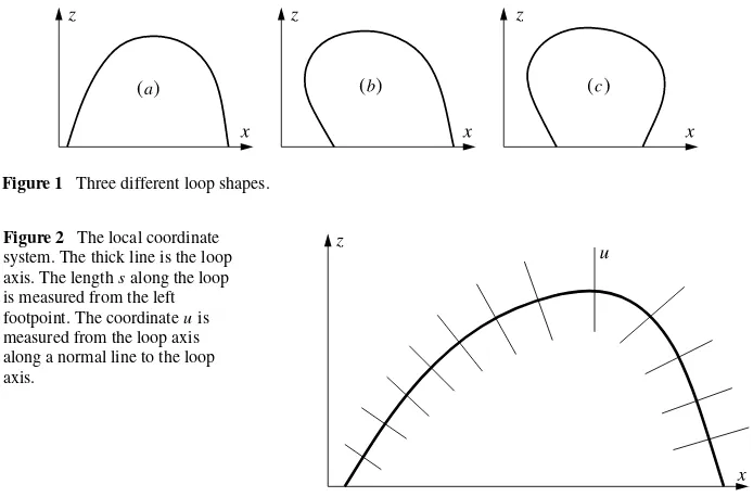
For simplicity, we assume below thatz0(s)monotonically increases in the interval(0, sa)
and monotonically decreases in the interval(sa, L), wheresacorresponds to the loop apex.
Figure 1 Three different loop shapes.
Figure 2 The local coordinate system. The thick line is the loop axis. The lengthsalong the loop is measured from the left footpoint. The coordinateuis measured from the loop axis along a normal line to the loop axis.
in the interval(s1, s2), and then again monotonically decreases in the interval(s2, L), where 0< s1< sa< s2< L. We also assume that the loop axis is a concave curve. The three pos-sible shapes of the loop are shown in Figures1a, b, and c. Other assumptions are that the distance between the loop footpoints is of the order ofL, and the smallest radius of the loop curvature is also of the order ofL.
3. Loop Cross-Section
We start by introducing a local curvilinear coordinate system in the vicinity of the loop axis. To do this, we draw straight lines normal to the loop axis at each point (see Figure2). We denote the length along a straight line measured from the point of its intersection with the loop axis asu. The quantity uis negative when it is measured inside the region bounded by the loop axis and the x-axis, and positive when it is measured outside. This is a local coordinate system because the normal lines, in general, intersect at some distance from the loop axis. However, we only use this coordinate system in the vicinity of the loop axis defined by the condition|u| ≤d. We show in AppendixAthat it is enough to impose the restriction thatdis smaller than half of the minimum curvature radius of the loop axis and also smaller than half of the distance between the loop footpoints. Hence, if we assume that these two quantities are much larger thanL, then we can takedmuch larger thanL. The equation of the normal line crossing the loop axis at the point(x0, z0)is
x=x0(s)−uz0(s), z=z0(s)+ux0(s). (5)
These equations give the relation between the curvilinear coordinates (s, u) and Carte-sian coordinates (x, z). Differentiating the identities x ≡x(s(x, z), u(x, z)) and z ≡ z(s(x, z), u(x, z))with respect toxandzyields
∂s ∂x =
1
∂z ∂u,
∂s ∂z= −
1
∂x ∂u,
∂u ∂x = −
1
∂z ∂s,
∂u ∂z =
1
∂x
where =∂x ∂s ∂z ∂u− ∂x ∂u ∂z
∂s. (7)
Using Equations (4) and (5), we obtain
=1−κu, κ=x0z0−x0z0, (8)
whereκis the loop-axis curvature. The curvature[κ]is positive if the tangent vector(x0, z0)
to the loop axis rotates counter-clockwise whensincreases and negative otherwise. It fol-lows from the assumption that the loop axis is a concave curve that its curvature is every-where negative.
With the aid of Equations (4), (5), and (8), we reduce Equation (6) to
∂s ∂x =
x0
1−κu,
∂s ∂z =
z0
1−κu,
∂u ∂x = −
z0+ux0 1−κu ,
∂u ∂z =
x0−uz0 1−κu .
(9)
Using Equation (8), we obtain
κ2=x0z0−x0z02=x02z02−2x0z0x0z0+x02z02. (10)
Now we use Equation (4) to transform this equation to
κ2=x0 2
+z0 2
−x0 2
x0 2
−2x0z0x0z0−z0 2
z0 2
=x0 2
+z0 2
−x0x0+z0z0
2
. (11)
In accordance with Equation (4), the second term on the right-hand side of this equation is zero, so eventually we arrive at
κ2=x02+z02. (12)
Using Equations (4), (8), (9), and (12), we rewrite Equation (2) in terms ofsanduas
∂ ∂s
1 1−κu
∂ψ ∂s + ∂ ∂u
(1−κu)∂ψ ∂u
=0. (13)
We look for the solution to this equation in the form of power series:
ψ=
∞
n=0
unψn(s). (14)
In what follows we assume that the loop axis is a magnetic-field line. This implies that
ψ=const. whenu=0. Without loss of generality, we can takeψ=0 whenu=0. Then
ψ0(s)=0. Now, substituting Equation (14) in Equation (13) and collecting terms with the same power ofu, we obtain the infinite set of equations for the coefficients ψn(s). It is
convenient to write the first two equations of this set separately. As a result, we have
2ψ2=κψ1, (15)
6ψ3=8κψ2−ψ1−2κ 2ψ
1, (16)
(n+1)(n+2)ψn+2=(n+1)(3n+1)κψn+1−ψn−n(3n−1)κ
2ψ
n
+κψn−1−κψn−1−(n−1)2κ3ψn−1, n=2,3, . . . (17)
We can see that we can takeψ1(s)arbitrarily and then calculateψn(s),n=2,3, etc., using
y0(s), andψ1(s)are sufficiently “good” functions, i.e. they satisfy all restrictions imposed in AppendixB, anddis sufficiently small, but still much larger thanL.
In what follows we use only the first non-zero term in the series in Equation (14) and assume that|u|L, so
ψ=uψ1(s)
1+O(). (18)
Consider the plane[]orthogonal to the loop axis at its left footpoint. Since the vector eu=(−z0(0), x0(0))is orthogonal to the loop axis at this footpoint[eu∈]. We denote
the unit vector in they-direction, which is the direction orthogonal to the plane of the loop, asey. Sinceeu⊥ey, these two vectors can be considered as the unit vector of Cartesian
coordinates in the plane[]. The corresponding coordinates areuandy, and the coordinate origin coincides with the intersection ofand the loop axis.
Now we consider a closed contour∈. It is defined by the equations
u=u0(t ), y=y0(t ), (19)
whereu0(T )=u0(0)andy0(T )=y0(0). We assume thatis a simple contour, i.e. it does not have self-intersections, and the coordinate origin is inside. In addition, we assume that
is convex, i.e. any straight line can intersect it at no more than two points. The numbers
u,y, andsdefine orthogonal curvilinear coordinates in three-dimensional space. In these coordinates the equation of the loop axis isu=y=0. The magnetic line crossing at a point with coordinates (u0(t ), y0(t ))is defined by the equationsy=y0(t )andψ (u, s)=
ψ (u0(t ),0). Varyingsfrom 0 toL, we obtain a part of this line bounded by the two planes orthogonal to the loop axis at the footpoints. Now we also varytfrom 0 toT. Then we obtain a magnetic surface consisting of magnetic lines crossing the contour. We can consider this surface as the surface of the magnetic tube. Then, using Equation (18), we write the equation of the surface of the magnetic tube as
y=y0(t ), uψ1(s)=u0(t )ψ1(0)
1+O(), 0≤s≤L,0≤t≤T . (20)
The boundary of the tube cross-section by the plane perpendicular to the tube axis ats= ¯s
is defined by the equation
y=y0(t ), u=u0(t )
ψ1(0)
ψ1(s)¯
1+O(), 0≤t≤T . (21)
We see that, in the leading-order approximation with respect to , the tube cross-section ats= ¯sis obtained from the tube cross-section ats=0 by stretching or compressing this latter cross-section in theu-direction with the coefficientψ1(0)/ψ1(s)¯ . In particular, if we taketo be a circle of radiusacentred at the loop axis, and we also takeψ1(s)≡1, then we obtain that in the leading-order approximation with respect to, the tube cross-section is the circle of radiusacentred at the loop axis everywhere. Hence, we can consider a planar loop of arbitrary shape and assume that it has a circular cross-section with constant radius everywhere.
4. Summary and Conclusions
In our analysis we assumed that the loop is embedded in a planar potential magnetic field. We also assumed that the loop axis is described by an analytical function. We showed that the loop cross-section can be prescribed arbitrarily at one of the loop footpoints. Then the loop cross-section at any other point is obtained by stretching or compressing the prescribed loop cross-section in the direction that is perpendicular to the loop axis and in the plane of the loop. The variation of the coefficient of stretching/compression along the loop can be chosen arbitrarily. Note that this result is only valid in the leading-order approximation with respect to the small parameter, which is the ratio of the characteristic size of the loop cross-section to the loop length.
In particular, it follows from the result we obtained that we can consider a planar loop of arbitrary shape and assume that its cross-section is circular everywhere and has a constant radius.
Acknowledgements The author acknowledges the support by an STFC grant (R/131168), and by the Rus-sian Fund for Fundamental Research (RFBR) grant (13-02-00656).
Open Access This article is distributed under the terms of the Creative Commons Attribution License which permits any use, distribution, and reproduction in any medium, provided the original author(s) and the source are credited.
Appendix A: Proof That the Map(s, u)→(x, z)Is Bijective
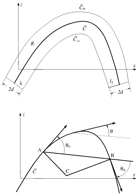
In this section we consider the map(s, u)→(x, z)defined by Equation (5). We slightly extend the curveC beyond the footpoints. This can be done in infinitely many ways. For example, we can use small arcs of circles of radii equal to the curvature radii at points
(x0(0),0)and(x0(L),0)(see Figure3). These circles are centred at the centres of curvature. The arc lengths are equal toδL. We denote the extended curve asC. Note that this curve is not only smooth, but it also has a continuous curvature. The lines normal toCat its end points have equations
x=x0(−δ)−uz0(−δ), z=z0(−δ)+ux0(−δ), (22)
x=x0(L+δ)−uz0(L+δ), z=z0(L+δ)+ux0(L+δ). (23)
We denote the first line as−and the second as+. Now we introduce two curvesC−and C+defined by the equations
x=x0(s)+dz0(s), z=z0(s)−dx0(s), s∈ [−δ, L+δ], (24)
x=x0(s)−dz0(s), z=z0(s)+dx0(s), s∈ [−δ, L+δ], (25)
respectively, whered is sufficiently small. The exact restriction ondwill be imposed later. Consider the rectangleDin the plane(s, u)defined by−δ < s < L+δ,|u|< d, and the domainRbounded by the lines−and+, and by the curves inC−andC+in the plane(x, z). Equation (5) defines a mapF:D→R.
First we show that the map F is injective. This means that F (sa, ua)=F (sb, ub) if (sb, ub)=(sa, ua). We assume the contrary, that there are two points, (sa, ua)∈D and (sb, ub)∈D, such thatF (sa, ua)=F (sb, ub)=(x, z). This implies that the two normal
lines to the curveC, one at point A and the other at point B, intersect at point C∈R, where A and B are the points on the curveC corresponding tos=sa ands=sb . Since C∈R,
Figure 3 Sketch of the domainR.
Figure 4 Illustration for the proof that the mapFis injective.
vector toC and the line AB connecting the points A and B (see Figure4). This angle takes the valuesθaandθbat points A and B. The distance between the points A and B is given by
|AB| =
sb
sa
cosθds. (26)
Using the relation dθ/ds=κ(s), we transform this expression to
|AB| =
θb
θa cosθ
κ dθ. (27)
Letκm=max|κ|fors∈ [−δ, L+δ]. Taking into account that−κm≤κ≤0 andθb<0, we
obtain from Equation (27) the estimate
|AB| ≥sinθa+sin|θb|
κm
= 2
κm
sinθa+ |θb| 2 cos
θa− |θb|
2 . (28)
It is straightforward to see that∠BAC=π/2−θa,∠ABC=π/2− |θb|, and, consequently, ∠ACB=θa+ |θb|. Then, using the law of sines, we obtain
cosθa
|BC| = cosθb
|AC| =
sin(θa+ |θb|)
Figure 5 Illustration of the proof that the mapFis injective for the case when the loop axis has the shape shown in Figure1b and the angle between the normals is larger thanπ.
Now we impose the restriction thatd <1/2κm. Since|AC|< d <1/2κmand|BC|< d <
1/2κm, it follows from Equation (29) that
|AB|< sin(θa+ |θb|) κm(cosθa+cosθb)
= sin
θa+|θb| 2
κmcosθa−|2θb|
. (30)
It follows from Equations (28) and (30) that 2 cos[(θa− |θb|)/2]<1 and, consequently,
cosθa− |θb|
<0. (31)
Since 0< θa≤π/2 and 0<|θb| ≤π/2, the inequality in Equation (31) cannot be satisfied,
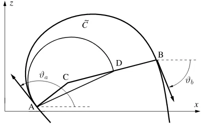
and we arrive at the contradiction. Hence, the normal lines at A and B cannot intersect inR. It is obvious that the proof presented above is only valid when the angle∠ACB is smaller thanπ. This is always true when the loop axis has the shape shown in Figure1a. However, when it has either the shape shown in Figure1b or that shown in Figure1c, it is also possible that∠ACB is larger thanπ. We consider the case shown in Figure1b and assume that the angle between the normal lines at A and B counted from the second line counter-clockwise is larger thanπ(see Figure5). Letϑ be the angle between the tangent toCand the positive
x-axis counted counter-clockwise from thex-axis. For the case shown in Figure1b,π/2< ϑa< πand−π/2≤ϑb≤0, so∠ACB=ϑa−ϑb<3π/2. We draw the arc AD of the circle
of radius 1/κmthat touches the curveC at A. This arc cannot cross C because otherwise
the absolute curvature ofC would have to exceedκmsomewhere between A and the point
of intersection. The second end of this arc cannot be on AC because, by assumption,|AC| is smaller than the half of the curvature radius. Since 2π−∠ACB>2π−3π/2=π/2, it follows that|AD|> (2/κm)sin(π/4)=
√
2/κm. Now we have
|AC| + |BC| ≥ |AC| + |CD|>|AD|>
√ 2
κm
, (32)
which again contradicts the assumption that C∈Rbecause, in that case, we would have |AC| + |BC|<2d <1/κm.
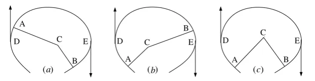
Finally, we consider a loop with the axis of the shape in Figure1c and assume that the angle between the normals is larger thanπ(see Figure6). At points D and E the tangents to the curveCare vertical. It is straightforward to see that if A is above D, as in Figure6a, or B is above E, as in Figure6b, then the proof is the same as for a loop with the axis of shape (b). Therefore we only need to consider the case where both A is below D and B is below E. Then it is obvious that|AC| + |BC|is larger than the distance between the end points of the curveC. We introducedf =x0(L)−x0(0). Then we have for the distance between the end points of the curveC
Figure 6 Illustration of the proof that the mapFis injective and has the shape shown in Figure1c and the angle between the normals is larger thanπ.
Now we impose the addition restrictiond < df/2−δ. Then we have that on the one hand
|AC| + |BC|> df −2δ, but on the other hand|AC| + |BC|<2d < df −2δ, and again we
arrive at the contradiction.
Hence, to summarize, we have proved that the mapFis injective ifd <min(1/2κm, df/
2−δ). To finish the proof that F is bijective, we now need to prove that for any point
(x, z)∈Rthere is a point(s, u)∈Dsuch thatF (s, u)=(x, z).
First of all, we note thatF can be extended on the closureDofD. Then it is straight-forward to see thatF is a bijection of the boundary ofDon the boundary ofR. Now we assume that there is point A∈Rsuch that no point fromDis mapped in A. There are two possibilities: Either there is a point in any vicinity of A that is the image of a point fromD, or there is a vicinity of A such that no point in this vicinity is the image of a point fromD.
Consider the first possibility. In this case, we can construct a sequence of points{An}
con-verging to A and such that, for each point An, there is point Bn∈Dsuch thatF (Bn)=An.
Since{An}is converging and||is bounded from below by a positive constant, it follows
that {Bn}is a Cauchy sequence and, consequently, it converges to a point B. SinceF is
continuous, it follows thatF (B)=A, and we arrive at a contradiction. Note that B is not at the boundary ofDbecause the boundary ofDis mapped into the boundary ofR.
Assume now that there is a vicinity [V] of A such that no point in this vicinity is an image of a point fromD. We consider a simple closed contour [L] enclosingVand such that each point of this contour is the image of a point fromD. Such a contour definitely exists. For example, we can take the boundary ofR. The contour [L] is the image of the contourS∈D,
F (S)=L. Now we contractS into a point. SinceF is continuous,Lalso has to contract into a point. During this process, a part ofLmust be inV. But this is impossible because, by assumption, no point inV is an image of a point fromD. Hence, we again arrive at a contradiction. As a result, we conclude that any point inRis an image of a point fromD, which means thatF is bijective.
Appendix B: Investigation of the Sum Convergence
In this appendix we study the convergence of the series in Equation (14). We assume that the functionsx0(s),y0(s), andψ (s)satisfy the inequalities
x0(m)(s)< Lh1−m, y0(m)(s)< Lh1−m, ψ1(m)(s)< C2h−2m, (34) where h1 and h2 are positive constants much larger thanL, C2 is a positive constant,
m=0,1, etc., andf(m)(s)denotes themth derivative of function f (s). First we assume
that these inequalities are valid fors∈ [0, L]. The first two inequalities in Equation (34)
larger than or equal toh1. At the end point of the interval we have to takes≥0 ands≤Lin these Taylor series. In AppendixAwe described one possible extension of functionsx0(s) andy0(s)using the arcs of circles. With the use of this extension we obtained the curveC that is smooth and curves continuously. In this section we use another extension of curveC. Using the expansion ofx0(s)andy0(s)in the infinite Taylor series at the end points of the interval[0, L], we can define them in the vicinities of pointss=0 ands=L. As a result, we obtain functionsx0(s)andy0(s)that are analytic in the interval(−δ, L+δ)for sufficiently small positiveδ. Hence, we obtain the analytic curveC.
It follows from the inequalities in Equation (34) that we can find such positive constants
handC,hbeing much larger thanL, that
κ(m)< h−m−1, ψ1(m)< Ch−m, m=0,1, . . . . (35) Now we prove that
ψn(m)< C(n/ h)m(5/ h)n−1, n=2,3, . . . , m=0,1, . . . . (36) It follows from Equation (15) that
2ψ2(m)= m
l=0
m
l
κ(l)ψ(m−l)
1 , (37)
wheremlis a binomial coefficient. Using Equation (35), we obtain from Equation (37)
ψ2(m)≤1
2
m
l=0
m
l κ
(l)ψ(m−l)
1 <
C
2hm+1
m
l=0
m
l
= 2mC 2hm+1<
5C h 2 h m . (38)
Hence, the inequality (36) is valid forn=2.
In what follows we need estimates for the derivatives ofκ2andκ3. We have
κ2(m)=
m
l=0
m
l
κ(l)κ(m−l). (39)
It follows from this equation and Equation (35) that
κ2(m)≤ m
l=0
m
l κ
(l)κ(m−l)< h−m−2
m
l=0
m
l
=2mh−m−2. (40)
Hence, eventually,
κ2(m)<1
4(2/ h)
m+2. (41)
Continuing, we obtain
κ3(m)=
m
l=0
m
l κ
2(l)
κ(m−l). (42)
Now using Equations (35) and (42) yields
κ3(m)≤ m
l=0
m
l κ
2(l)
κ(m−l)<1
4
m
l=0
m
l
2
h l+2
hl−m−1
=h−m−3 m
l=0
m
l
Hence, eventually we obtain
κ3(m)< 1
27(3/ h)
m+3. (44)
Differentiating Equations (16) yields
6ψ3(m)=8
m
l=0
m
l
κ(l)ψ2(m−l)−ψ1(m+2)−2
m
l=0
m
l κ
2(l)
ψ1(m−l). (45)
Then, using Equations (35), (41), and (44), and Equation (36) withn=2, we obtain
ψ3(m)≤ m
l=0
m
l
4 3κ
(l)ψ(m−l)
2 +
1 3κ
2(l) ψ1(m−l)
+1 6ψ
(m+2)
1
< C hm+2
m
l=0
m
l
20 3 2
m−l+1
32 l +1 6 = C
hm+2
7·3m+1 6 < C 3 h m 5 h 2 . (46)
Hence, we see that the inequality (36) is valid forn=3. Now we use the method of math-ematical induction. Assume that the inequalities (36) are valid for 2≤n≤k, wherek≥3, and prove that they are then also valid forn=k+1. It follows from Equation (17) with
n=k−1 that
k(k+1)ψk+1=k(3k−2)κψk−ψk−1−(k−1)(3k−4)κ2ψk−1
+κψk−2−κψk−2−(k−2)2κ3ψk−2. (47) Differentiating this equation yields
k(k+1)ψk(m)+1= m
l=0
m
l k(3k−2)κ (l)ψ(m−l)
k +κ
(l)ψ(m−l+2) k−2
−(k−1)(3k−4)κ2(l)ψk(m−−1l)−κ(l+1)ψk(m−−2l+1)
−(k−2)2κ3(l)ψk(m−−2l+1)−ψk(m−+12). (48) It follows from Equations (35), (41), (44), (48), and the assumption that the inequalities (36) are valid forn≤kthat
k(k+1)ψk(m)+1≤ m
l=0
m
l k(3k−2)κ
(l)ψ(m−l)
k +κ(l)ψ (m−l+2) k−2
+(k−1)(3k−4)κ2(l)ψk(m−−1l)+κ(l+1)ψk(m−−2l+1)
+(k−2)2κ3(l)ψk(m−−2l)+ψk(m−+12)
< C hm+k
m
l=0
m
l k(3k−2)5
k−1km−l+(k−2)25k−3(k−2)m−l
+(k−1)(3k−4)5k−22l(k−1)m−l+(k−2)5k−3(k−2)m−l
+(k−2)25k−33l(k−2)m−l+C(k−1)m+25k−2h−m−k
= C hm 5 h k
(k+1)m
k(3k−2)
5 +
(k−1)(4k−5)
25 +
2(k−2)2 125
+(k−1)m
(k−1)2
25 +
(k−2)2+k−2 125
< C
k+1
h
m5
h
k97k2−96k+40
125 < k(k+1)C
k+1
h
m5
h k
.
(49)
Hence, we have proved that the inequalities (36) are valid for n≤k+1. In accordance with the mathematical induction, this means that they are valid for anyn. It follows from the inequality (36) that the series in Equation (14) as well as any series obtained from this series by term-by-term differentiatingmtimes with respect tos andl times with respect tou, wheremandl are any non-negative integer numbers, are convergent with the radius of convergence larger than or equal to h/5. Sinceh is of the order of L, this radius of convergence is much larger thanL.
References
Andries, J., Arregui, I., Goossens, M.: 2005, Astrophys. J. Lett. 624, L57.DOI.
Andries, J., Van Doorsselaere, T., Roberts, B., Verth, G., Erdélyi, R.: 2009, Space Sci. Rev. 149, 3.DOI. Aschwanden, M.J.: 2006, Phil. Trans. Roy. Soc. A 364, 417.DOI.
Aschwanden, M.J., Schrijver, C.J.: 2011, Astrophys. J. 736, 102.DOI.
Aschwanden, M.J., Fletcher, L., Schrijver, C.J., Alexander, D.: 1999, Astrophys. J. 520, 880.DOI. Aschwanden, M.J., De Pontieu, B., Schrijver, C.J., Title, A.M.: 2002, Solar Phys. 206, 99.DOI. Dymova, M., Ruderman, M.S.: 2005, Solar Phys. 229, 79.ADS.DOI.
Dymova, M., Ruderman, M.S.: 2006, Astron. Astrophys. 459, 241.DOI. Edwin, P.M., Roberts, B.: 1983, Solar Phys. 88, 179.DOI.
Morton, R.J., Erdélyi, R.: 2009, Astron. Astrophys. 502, 315.DOI. Morton, R.J., Ruderman, M.S.: 2011, Astron. Astrophys. 527, A53.DOI.
Nakariakov, V., Ofman, L., DeLuca, E.E., Roberts, B., Davila, J.M.: 1999, Science 285, 862.DOI. Orza, B., Ballai, I.: 2013, Astron. Nachr. 334, 948.DOI.
Ruderman, M.S.: 2003, Astron. Astrophys. 409, 287.DOI. Ruderman, M.S.: 2009, Astron. Astrophys. 506, 885.DOI. Ruderman, M.S., Erdélyi, R.: 2009, Space Sci. Rev. 149, 199.DOI. Ruderman, M.S., Verth, G., Erdélyi, R.: 2008, Astrophys. J. 686, 694.DOI. Ryutov, D.D., Ryutova, M.P.: 1976, Sov. Phys. JETP 43, 491.ADS. Schrijver, C.J., Brown, D.S.: 2000, Astrophys. J. Lett. 537, L69.DOI.
Schrijver, C.J., Aschwanden, M.J., Title, A.M.: 2002, Solar Phys. 206, 69.DOI. Terradas, J., Oliver, R., Ballester, J.L.: 2006, Astrophys. J. Lett. 650, L91.DOI.
Van Doorsselaere, T., Debosscher, A., Andries, J., Poedts, S.: 2004, Astron. Astrophys. 424, 1065.DOI. Van Doorsselaere, T., Verwichte, E., Terradas, J.: 2009, Space Sci. Rev. 149, 299.DOI.