Induced Topological Phases at the Boundary of 3D Topological Superconductors

This is a repository copy of

Induced Topological Phases at the Boundary of 3D Topological

Superconductors

.

White Rose Research Online URL for this paper:

http://eprints.whiterose.ac.uk/99990/

Version: Accepted Version

Article:

Finch, P, de Lisle, J, Palumbo, G et al. (1 more author) (2015) Induced Topological Phases

at the Boundary of 3D Topological Superconductors. Physical Review Letters, 114 (1).

016801. ISSN 0031-9007

https://doi.org/10.1103/PhysRevLett.114.016801

[email protected] https://eprints.whiterose.ac.uk/

Reuse

Unless indicated otherwise, fulltext items are protected by copyright with all rights reserved. The copyright exception in section 29 of the Copyright, Designs and Patents Act 1988 allows the making of a single copy solely for the purpose of non-commercial research or private study within the limits of fair dealing. The publisher or other rights-holder may allow further reproduction and re-use of this version - refer to the White Rose Research Online record for this item. Where records identify the publisher as the copyright holder, users can verify any specific terms of use on the publisher’s website.

Takedown

If you consider content in White Rose Research Online to be in breach of UK law, please notify us by

Peter Finch, James de Lisle, Giandomenico Palumbo, and Jiannis K. Pachos School of Physics and Astronomy, University of Leeds, Leeds, LS2 9JT, United Kingdom

We present tight-binding models of 3D topological superconductors in class DIII that support a variety of winding numbers. We show that gapless Majorana surface states emerge at their boundary in agreement with the bulk-boundary correspondence. At the presence of a Zeeman field the surface states become gapped and the boundary behaves as a 2D superconductor in class D. Importantly, the 2D and 3D winding numbers are in agreement signifying that the topological phase of the boundary is induced by the phase of the 3D bulk. Hence, the boundary of a 3D topological superconductor in class DIII can be used for the robust realisation of localised Majorana zero modes.

PACS numbers: 73.20.At, 74.20.Rp, 03.65.Vf, 71.10.Pm, 74.90.+n

Introduction:–1D and 2D tight-binding topological superconductors (TS) are a commonly employed medium to probe localised Majorana zero modes (Majoranas) with non-Abelian statistics. 1D tight-binding TS are em-ployed to theoretically investigate the properties of Ma-joranas and experimentally verify their existence [1]. 2D tight-binding TS provide exactly solvable models, where Majoranas exhibit rich behaviour [2–4]. Despite the suc-cess of these models little work has been done in relation to 3D tight-binding TS [5, 6].

Here we consider a general class of 3D tight-binding models of fermions positioned at the vertices of a cu-bic lattice. We allow for tunnelling and pairing inter-actions between nearest and next-to-nearest neighbour-ing sites of the lattice. When we impose time-reversal (TR) and particle-hole (PH) symmetries we obtain ex-plicit realisations of 3D TS of type DIII [7]. For pe-riodic boundary conditions in all three directions we provide a variety of TS that support winding numbers

ν3D = 0,±1,±2,±3,±4. Similar models that exhibit

ν3D = ±2 [9] and ν3D = ±1 [10] and higher [11] have recently been presented. In our model, the higher values of ν3D are obtained while keeping fixed the size of the unit cell and the range of interactions. Subsequently, we impose open boundary conditions in one direction and identify edge modes with dispersion relation that crosses the band gap [12], which correspond to gapless Majo-rana surface states. These states acquire a gap when a Zeeman field is applied at the boundary that breaks TR symmetry [13–15]. Thus, the boundary behaves as a TS of the class D. It is known that both the 3D class DIII and the 2D class D TS have a Z _{topological invariant}

[7]. Here we show that under certain conditions the ac-tual values of these topological invariants that describe the bulk and the boundary physics of a 3D class DIII TS are equal. We demonstrate this both numerically, for all the tight-binding models presented here, and theoret-ically, based on an effective topological field theory. This protection of the boundary topological phase from the topological character of the bulk provides the means for the fault-tolerant realisation of localised Majoranas [16]. These Majoranas can be employed for topological

quan-tum computation [17] that is resilient against erroneous perturbations or thermal fluctuations.

DIII lattice:– We now introduce the lattice model. We consider two species of fermion, a1 and a2, canon-ically ordered on a cubic lattice, as shown in Fig. 1 (Left). The unit cell, positioned at j= (jx, jy, jz), con-sists of two sites lying along thex-axis. The Hamiltonian is given by

H =X j

X

k

µa†_kjakj+

X

k,k′_,s

tkk′sa†_kjak′_j+s

+ X

k,k′,s

∆kk′sakjak′j+s

+ h.c., (1)

wheretkk′sand ∆kk′s are the tunnelling and pairing cou-plings, respectively, µis the chemical potential and sis a vector connecting interacting unit cells. The interac-tions are taken to be at most between next-to-nearest neighbours. For periodic lattice we introduce the Fourier transformation ak,j = Ppeip·jak,p to obtain H =

P

pψp†h(p)ψp, where ψp = (a1,p, a†1,−p, a2,p, a†2,−p)T, p_∈BZ = [0,2π)×[0,2π)×[0,2π) and the kernelh(p) is a 4×4 hermitian matrix. To impose TR and PH sym-metries we introduce the unitary operatorsCTRandCPH and demand that

C_TR† h∗_(−p)C

TR=h(p), CPH† h∗(−p)CPH=−h(p) (2)

withCT

TR=−CTRandCPHT =CPH. These requirements guarantee that our model belongs in class DIII. Next we interpret the species index k = 1,2 as spin-1/2 compo-nents. For simplicity we unitarily rotate the Hamiltoni-ans into the basis ˜ψp= (ia1,p−a†1,−p, a2,p−ia†2,−p, ia1,p+

a†1,−p, a2,p+ia†2,−p)T/ √

2 such that the kernel takes the spin-triplet TS form [20, 21]

h(p) =

ǫ(p)I _Θ(p) Θ(p)† _−ǫ(p)I

, (3)

with ǫ(p) denoting the normal state, I _{is the identity}

2

−5 0 5

∆ −5

0 5

µ

0 1 2

FIG. 1: (Colour online) (Left) The lattice onto which the fermions are placed. The unit cell (dashed square) consists of two fermions a1 (white site) and a2 (black site). Tun-nelling and pairing interactions are assumed between nearest and next-to-nearest neighbouring sites. (Right) The energy gap minp(|E(p)|) as function ofµ and ∆ when t = 1. The winding number is depicted as a function of µ and ∆ tak-ing valuesν3D= 0,±1. Changes in the winding number are accompanied by quantum phase transitions.

matrices andd(p) = (dx(p), dy(p), dz(p)) are odd func-tions. The corresponding doubly degenerate spectrum is given byE(p) =±pǫ(p)2_+|d(p)|2_{. We take the system} to be prepared in its lowest energy, where both negative valance bands are completely occupied. The topological nature of the gapped regions is identified by the winding numberν3D∈Zthat characterises the mapping between the toroidal Brillouin zoneT3 _{and the sphereS}3_defined by the normalised 4D vector (ǫ(p),d(p))/|E(p)|. This can be evaluated in terms of projectors to the two lowest eigenstates of kernel (3) [7].

We now take a specific coupling configuration that gives rise to a non-trivial winding number. More con-cretely, for a particular set of interactions {s_} we can have ǫ(p) = t[cos(px − pz) + cos(px) + 2 cos(py −

pz) + cos(py)]−µ, dx(p) = ∆[sin(px−pz) + sin(px) + 2 sin(py−pz)−sin(py)],dy(p) = 2∆ sin(py) anddz(p) = 2∆ sin(px+py) with t, µ,∆ ∈ R. This corresponds to a mixture of s and p wave pairing without spin-orbit interactions [8]. The energy gap as function of µ and ∆ for t = 1 as well as the winding number, ν3D, cor-responding to each gapped phase are shown in Fig. 1 (Right). It is possible to evaluate the winding number in terms of the set of momentap∗ satisfyingd(p∗) = 0 fromν3D= 12

P

d(p∗₎₌₀sgn[ǫ(p∗)]sgn{det[∂jdi(p∗)]}[21]. This expression shows explicitly the dependence of its sign, sgn(ν3D), in terms of the product of the signs of the couplings ∆ andµ, as shown in Fig. 1 (Right).

Boundary properties:–Let us now consider the case where a boundary is introduced in the model defined above. For concreteness we take the lattice to extend be-tween two disconnected planes. The Bottom plane (B) positioned atz= 1 and the Top plane (T) positioned at

z =l, wherel is a positive integer. The Hamiltonian of

−π

2 0

π

2

px −10

0 10

E

−π

2 0

π

2

px −10

0 10

∆_E

0 0 0.5

By

∆E

0.5

FIG. 2: (Left) An energy dispersion cross section atpy= 0

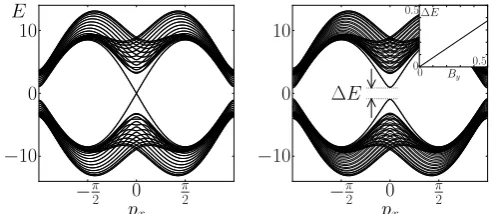
for the ν3D = 1 model (t = 1, ∆ = 2, µ = 3) with open boundaries atz = 1 andz = 20. A single cone appears with a double degeneracy corresponding to the two Majorana edge modes, one for each surface. (Right) A boundary Zeeman field withBy 6= 0 generates an energy gap, ∆E, to the edge

modes. (Inset) The energy gap ∆Eas a function ofBy.

the system with a boundary is given by

H = X

¯ p,z,s

ψ†z,p¯h(¯p;z,z+s)ψz+s,¯p

+X

¯ p

ψ†1,p¯hBψ1,¯p+ψ

†

l,¯phTψl,p¯

(4)

where ψz,¯p = (a1,z,p¯, a

†

1,z,−p¯, a2,z,¯p, a

†

2,z,−p¯)T with z a vector in thez-direction, ¯p_∈[0,2π)×[0,2π) the momen-tum on thex–y plane. We write the boundary Hamil-tonian in this basis to ease the subsequent discussion of the physics of the boundary fields. The hB and hT terms are interactions corresponding to the Bottom and Top planes, respectively. These terms are introduced to give an energy gap to the boundary states and do not affect the properties of the bulk. While it is pos-sible to consider independent interaction terms at each plane, for uniformity we choose them to be equal, given byhT =hB =B·σ⊗I, whereBis a 3D vector. These terms can be viewed as an effective Zeeman field that breaks time reversal symmetry. They correspond to in-teractions between the fermionic modesa1anda2within the same unit cell.

num-ber in terms of the projectors onto these gapped surface states [18, 19]. For N such states with the same helic-ity the winding number is given by νb = ±N/2 where

b=T, B, that we call partialwinding number. The sign ofνbdepends on the helicity of the edge states as well as the sign ofBy that generates their gap.

While each plane constituting the boundary can be treated independently, the condition hT =hB allows us to consider the entire boundary as a 2D TS dislocated between the two planes. The effective Hamiltonian that describes the low energy limit of these 2D superconduct-ing states breaks TR symmetry, due to the presence of non-zeroBy, so it behaves as a class D system [7]. Sub-sequently, we can define the sum of the partial winding numbers,ν2D=P_bνb, which characterises the topologi-cal phase of the boundary as a whole.

We would now like to see how the winding number

ν2D of the boundary relates to the winding numberν3D of the bulk when both bulk and boundary are gapped. To make the comparison legitimate we choose ∆, the order parameter of the bulk, andBy, the order parameter of the boundary, to have the same sign, i.e. sgn(By) = sgn(∆). Let us first look at theν3D = 0 case. We find that each plane supports two pairs of Majorana edge modes with opposite helicities. As a result the 2D winding number is ν2D = 0. When ν3D = 1 each plane supports N = 1 Majorana cone. When gapped, each partial winding number contributesνb= 1/2 to the 2D winding number, such thatν2D= 1. A similar result holds whenν3D=−1. In analogy to the 2D SC in class D [16] we expect that when ν3D =±1 the boundaries can support Majoranas localised at the endpoints of vortex strings that terminate on the boundaries [22].

Higher winding numbers:–We now present models that support higher winding numbers without the need to increase the size of the unit cell or the range of inter-actions. These models are obtained by searching among a variety of possible configurations of interactions that respect the TR and PH symmetries (2), so they are in class DIII. Using the notation of (3), we present Hamilto-nianH2withǫ(p) =t[cos(px)+cos(px−pz)]−µ,dx(p) = ∆[sin(px)+sin(px−pz)],dy(p) = 2∆ sin(py) anddz(p) = 2∆ sin(px +py) that supports topological phases with

ν3D= 0,±2, HamiltonianH3withǫ(p) =−t[−cos(px) + cos(px−pz)+cos(2py)−cos(py+pz)+cos(py)]+µ,dx(p) = ∆[−sin(px)−sin(px−pz) + sin(2py)−sin(py)−sin(py−

pz)], dy(p) = 2∆ sin(py) and dz(p) = 2∆ sin(px−py) that supportsν3D= 0,±1,±3 and HamiltonianH4 with

ǫ(p) =t[cos(px+pz)−2 cos(py)]+µ,dx(p) =−∆ sin(px+

pz), dy(p) = −2∆ sin(pz) and dz(p) = 2∆ sin(px+py) that supportsν3D= 0,±2,±4.

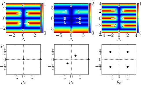
The phase diagrams of the H2, H3 and H4 models are shown in Fig. 3 (Top Row). In each case, multiple gapped topological phases are separated by gapless phase transitions. We then introduce open boundary conditions in thez-direction and observe gapless Majorana states

lo-−2 0 2 ∆ −2 0 2 µ 0 1

−5 0 5 ∆ −5 0 5 0 2

−4 ₋2 0 2 4 ∆ −4 −2 0 2 4 0 1 −π 2 0 π 2 px −π 2 0 π 2 py

.

.

.

. .

.

. .

.

FIG. 3: (Colour online) (Top Row) The energy gaps ofH2,H3 andH4, ordered from left to right, as a function ofµand ∆ fort= 1. The winding number associated with each gapped phase is indicated. (Bottom Row) The centre of the surface Majorana cones are given for the model corresponding to the gap diagram above it, when each model is in the max(ν3D) phase. All plots were generated withµ= 0.1, ∆ =t= 1.

calised at each surface. When the winding numberν3Dis non-zero we find that for all modelsN =|ν3D|many such surface states exist at each edge with the same helicity. Next we consider each model in the phase with max(ν3D). The position of the zero energy points of their Majorana edge states is shown in Fig. 3 (Bottom Row). A pair of Majorana modes (one per edge) corresponds to each dot in the Figure. Finally, we introduce a boundary Zeeman field withBy 6= 0. We numerically find that for all cases the induced 2D winding number satisfiesν2D =ν3D. In other words, if a phase transition in the bulk occurs such that the new phase has a different 3D winding number, then the number and/or helicity of Majorana cones on the boundary and the 2D winding number change ac-cordingly.

Bulk-boundary correspondence:– The bulk-boundary correspondence witnessed here as the agreement between ν2D and ν3D is not accidental. We now present an analytic link between these two topological invariants by looking at the thermal Hall conductivity (THC). In particular, we establish a rela-tionship between the THC of a 2D TS in the class D, that is proportional toν2D, and the THC induced on the boundary (composite system of two surfaces) of a 3D TS in the class DIII, that is shown to be proportional to

ν3D.

The thermal properties of TS can be encoded in an effective topological field theory (ETFT) obtained by in-troducing a fictitious gravitational field, as described by Luttinger theory [23]. In the 2D class D model, the ETFT is a gravitational Chern-Simons theory as showed in [16, 24] (see also (8) below). From this description and from independent arguments [25] it was possible to show that the THC is given by κ2D

th = ν C

4

TS (ℏ_{=kB= 1). In our case, the THC of the composite}

boundary of the 3D TS is the sum of the THC of the two surfaces, thus we have

κboundary_th = ν2D

12 π T, (5)

whereν2D=νT+νB.

We now calculate the boundary THC in an alternative way, by starting from the 3D bulk properties. The 3D model (1) of a certain topological phase can be adiabati-cally connected to a model with a low energy description given by massive Dirac fermions [26] with action

Sψ=

Z

M

d4_{xψ γ¯} µ_∂

µ+mψ, (6)

whereµ= 0,1,2,3, ¯ψ=γ0_{ψ, γ}µ _{are the Dirac matrices} andM is the (3 + 1)-dimensional spacetime. In order to calculate the ETFT, we introduce a curved background to the fermionic actionSψ. This is done by coupling the fermions with spin connection,ωµ, and tetrads that nat-urally encode the geometric properties of curved spaces [27]. The effective action Seff that describes the model purely in terms of the spin connection can be derived by integrating out the fermions in the corresponding parti-tion funcparti-tion. The topological part ofSeff that faithfully describes the low-energy behaviour of the model is given by [28, 29]

S_effM,top=1 2

θ

768π2

Z

M

d4_{x ǫ}µναβ_tr(Rρ

σµνRραβσ ), (7)

whereRρ

σµν is the Riemann tensor given in terms of the spin connection ωµ, while θ =ν3Dπ mod 2π [30]. This is the ETFT of the 3D TS. The topological behaviour of the gapped boundary can be obtained from (7) by considering that the spatial part ofM has a non-empty boundary with spacetime boundary manifold given by

∂M. By applying Stokes’ theorem we have

Seff∂M,top = 1 2

θ

192π2

Z

∂M

d3x ǫµνλtrωµ∂νωλ+ 2

3ωµωνωλ

.

(8) The action Seff∂M,top corresponds to the gravitational Chern-Simons theory. By general arguments [16, 28, 29] one can connect the coefficient of this Chern-Simons the-ory to the THC on the boundary of a 3D TS. In our sys-tem the boundary consists of two disconnected surfaces, the Top and the Bottom. Therefore the total boundary THC,κboundary_th , is given by

κboundary_th = 2×ν₂₄3Dπ T. (9)

Comparing equations (5) and (9), we deduce that

ν3D=ν2D (10)

as it was also numerically verified for all the presented models. Note that a relative sign freedom in (10) is

possible due to the orientation of the boundary surface employed during the application of the Stokes’ theorem. This is the geometric equivalent of the freedom we had in choosing the sign ofBy.

Protected 2D topological phases:– We have pre-sented 3D TS models in class DIII that exhibit a large variety of winding numbersν3D= 0,±1,±2,±3,±4. Nu-merical and theoretical analysis showed that the bound-ary of these models behaves as a 2D TS of class D with winding number ν2D = ν3D. Nevertheless, there is an intriguing difference between the boundary of a 3D TS and a purely 2D TS system. In the 3D case the 2D topological boundary isdelocalisedbetween two spatially separated surfaces [31]. In the limit of an infinitely thin bulk the two surfaces combine and we retrieve the con-ventional class D superconductor. Non-local encoding of the topological phase, together with relation (10), pro-vide a protection that is not present in the purely 2D system, as we analyse below.

Firstly, external perturbations cannot affect the topo-logical nature of the boundaries. As an adversary mech-anism consider placing on aνb = 1/2 edge another 2D lattice system with Chern numberνCh = ±1. The lat-ter can be effectively described by two massive Majorana fermions [2]. Perturbative interactions between this sys-tem and the edge can cause the edge Majorana fermion to pair with one of the Majorana fermions of the ap-pended system creating a non-topological Dirac fermion [32]. This leaves behind an edge with a single Majorana fermion that is still described byνb =±1/2, where one can easily compensate for a change in the sign. In par-ticular, this mechanism cannot causeνb to become zero. Secondly, phase transitions due to a thermal environ-ment are suppressed at low enough temperatures. Let us consider local thermal fluctuation at the boundary of the TS manifested as a vortex string in the bulk with both endpoints (a vortex-antivortex pair) residing on the same surface. As these endpoints bear localised Majoranas, a finite density of such thermal errors could cause a quan-tum phase transition due to vortex nucleation [33, 34]. Nevertheless, these vortex strings have a finite energy per string length that generates a string tension [35]. As a consequence, the vortex and the antivortex will be at-tracted to each other and annihilate, thus self-correcting the thermal error [36]. Only vortex strings with end-points at opposite surfaces can be stable [37, 38]. Hence, for low enough temperatures, the vortex string tension will cause the density of vortices on the surface to be zero, and its topological phase will remain intact. A re-cent study on the protection of the surface topological phase against weak interactions and disorder is given in [39, 40]. These error-resilience characteristics make the boundaries of 3D class DIII TS a promising laboratory for performing topological quantum computation [17].

dis-cussions. This work was supported by EPSRC.

[1] A. Y. Kitaev, Phys.-Usp.44_{, 131 (2001).}

[2] A. Y. Kitaev, Ann. Phys.321_{, 1 (2005).}

[3] V. Lahtinen, G. Kells, A. Carollo, T. Stitt, J. Vala and J. K. Pachos, Ann. Phys.323_{, 9 (2008).}

[4] V. Lahtinen and J. K. Pachos, New J. Phys.11_{, 093027}

(2009) .

[5] S. Ryu, Phys. Rev. B79_{075124 (2009).}

[6] Z. Nussinov, G. Ortiz and E. Cobanera, Phys. Rev. B

86_{, 085415 (2012).}

[7] A. P. Schnyder, S. Ryu, A. Furusaki and A. W. W. Lud-wig, Phys. Rev. B78_{, 195125 (2008).}

[8] J. K. Pachos, E. Alba, V. Lahtinen and J. J. Garcia-Ripoll, Phys. Rev. A 88_{, 013622 (2013).}

[9] A. P. Schnyder, S. Ryu and A. W. W. Ludwig, Phys. Rev. Lett. 102_{, 196804 (2009).}

[10] L. Fu and E. Berg, Phys. Rev. Lett.105_{, 097001 (2010).}

[11] D.-L. Deng, S.-T. Wang and L.-M. Duan, Phys. Rev. B

89_{, 075126 (2014).}

[12] M. Z. Hasan and C. L. Kane, Rev. Mod. Phys.82_{, 3045}

(2010).

[13] M. Sato, Y. Takahashi and S. Fujimoto, Phys. Rev. Lett.

103_{, 020401 (2009).}

[14] J. Alicea, Phys. Rev. B81_{, 125318 (2010).}

[15] L. Fu and C. L. Kane, Phys. Rev. Lett. 100_{, 096407}

(2008).

[16] N. Read and D. Green, Phys. Rev. B61_{, 10267 (2000).}

[17] J. K. Pachos,Topological Quantum Computation, Cam-bridge University Press (2012).

[18] D. J. Thouless, M. Kohmoto, M. P. Nightingale, and M. den Nijs, Phys. Rev. Lett.49_{, 405 (1982).}

[19] J. de Lisle, S. De, E. Alba, A. Bullivant, J. J. Garcia-Ripoll, V. Lahtinen and J. K. Pachos, to appear in NJP, arXiv:1402.3222 (2014).

[20] M. Sigrist and K. Ueda, Rev. Mod. Phys.63_{, 239 (1991).}

[21] M. Sato, Phys. Rev. B79_{, 214526 (2009).}

[22] J. C.Y. Teo and C.L. Kane, Phys. Rev. Lett.104_{, 046401}

(2010).

[23] J. M. Luttinger, Phys. Rev.135_{, A1505 (1964).}

[24] G. E. Volovik, JETP Lett.51_{, 125 (1990).}

[25] H. Sumiyoshi and S. Fujimoto, J. Phys. Soc. Jpn.82_,

023602 (2013).

[26] S. Ryu, A. P. Schnyder, A. Furusaki and A. W. W. Lud-wig, New J. Phys.12_{, 065010 (2010).}

[27] We apply the following substitutions in the action (6): ∂µ → ∂µ+ωµ,γµ → γαeµα, d

4

x→ d4x|e| withα, β = 0,1,2,3, where ωµ = 4iω

αβ

µ [γα, γβ] is the spin

connec-tion,eµ

α are the tetrads and |e|is the corresponding

de-terminant. In particular, we have that gµν = eαµeβνηαβ

where gµν is the metric tensor and ηαβ the Minkowski

one, while the spin connection has the Levi-Civita form: ωαβµ =eαν▽µeβν, where▽µ=eλµ(∂λ+ωλ).

[28] Z. Wang, X.-L. Qi and S.-C. Zhang, Phys. Rev. B84_,

014527 (2011).

[29] S. Ryu, J. E. Moore and A. W. W. Ludwig, Phys. Rev. B85_{, 045104 (2012).}

[30] Z. Wang and S.-C. Zhang, Phys. Rev. B 86_{, 165116}

(2012).

[31] One can shrink the bulk of the examples given above so that the two planes of the boundary are on the top of each other. This process can happened adiabatically, connect-ing the topological surface system to the correspondconnect-ing 2D system.

[32] B. A. Bernevig and T. L. Hughes, Topological Insula-tors and Topological SuperconducInsula-tors, Princeton Univer-sity Press (2013).

[33] V. Lahtinen, A. W. W. Ludwig, J. K. Pachos and S. Trebst, Phys. Rev. B86_{, 075115 (2012).}

[34] B. Bauer, R. M. Lutchyn, M. B. Hastings and M. Troyer, Phys. Rev. B87_{, 014503 (2013).}

[35] M. Eto, Y. Hirono, M. Nitta, and S. Yasui, Prog. Theor. Exp. Phys. 012D01 (2014).

[36] A. M. J. Schakel, Phys. Rev. E63_{, 026115 (2001).}

[37] P. Hosur, P. Ghaemi, R. S. K. Mong, and Ashvin Vish-wanath, Phys. Rev. Lett.107_{, 097001 (2011).}

[38] H.-H. Hung, P. Ghaemi, T. L. Hughes and M. J. Gilbert, Phys. Rev. B87_{, 035401 (2013).}

[39] M. S. Foster, H.-Y. Xie and Y.-Z. Chou, Phys. Rev. B

89_{, 155140 (2014).}

[40] D. Roy, N. Bondyopadhaya and S. Tewari, Phys. Rev. B