adaptive remeshing
.
White Rose Research Online URL for this paper:
http://eprints.whiterose.ac.uk/84567/
Version: Published Version
Article:
Hill, J orcid.org/0000-0003-1340-4373, Popova, E E, Ham, D A et al. (2 more authors)
(2014) Adapting to life : ocean biogeochemical modelling and adaptive remeshing. Ocean
Science. pp. 323-343. ISSN 1812-0784
https://doi.org/10.5194/os-10-323-2014
[email protected] https://eprints.whiterose.ac.uk/ Reuse
Items deposited in White Rose Research Online are protected by copyright, with all rights reserved unless indicated otherwise. They may be downloaded and/or printed for private study, or other acts as permitted by national copyright laws. The publisher or other rights holders may allow further reproduction and re-use of the full text version. This is indicated by the licence information on the White Rose Research Online record for the item.
Takedown
If you consider content in White Rose Research Online to be in breach of UK law, please notify us by
www.ocean-sci.net/10/323/2014/ doi:10.5194/os-10-323-2014
© Author(s) 2014. CC Attribution 3.0 License.
Ocean Science
e
n
Acce
ss
Adapting to life: ocean biogeochemical modelling and adaptive
remeshing
J. Hill1, E. E. Popova2, D. A. Ham3, M. D. Piggott1,4, and M. Srokosz2
1Applied Modelling and Computation Group, Department of Earth Science and Engineering, Imperial College London, SW7 2AZ, UK
2National Oceanography Centre, Southampton, University of Southampton Waterfront Campus, European Way, Southampton, SO14 3ZH, UK
3Applied Mathematics and Mathematical Physics, Department of Mathematics, Imperial College London, SW7 2AZ, UK 4Grantham Institute for Climate Change, Imperial College London, SW7 2AZ, UK
Correspondence to: J. Hill ([email protected])
Received: 23 September 2013 – Published in Ocean Sci. Discuss.: 5 November 2013 Revised: 30 March 2014 – Accepted: 1 April 2014 – Published: 9 May 2014
Abstract. An outstanding problem in biogeochemical
mod-elling of the ocean is that many of the key processes oc-cur intermittently at small scales, such as the sub-mesoscale, that are not well represented in global ocean models. This is partly due to their failure to resolve sub-mesoscale phenom-ena, which play a significant role in vertical nutrient supply. Simply increasing the resolution of the models may be an inefficient computational solution to this problem. An ap-proach based on recent advances in adaptive mesh compu-tational techniques may offer an alternative. Here the first steps in such an approach are described, using the example of a simple vertical column (quasi-1-D) ocean biogeochemi-cal model.
We present a novel method of simulating ocean biogeo-chemical behaviour on a vertically adaptive computational mesh, where the mesh changes in response to the biogeo-chemical and physical state of the system throughout the sim-ulation. We show that the model reproduces the general phys-ical and biologphys-ical behaviour at three ocean stations (India, Papa and Bermuda) as compared to a high-resolution fixed mesh simulation and to observations. The use of an adap-tive mesh does not increase the computational error, but re-duces the number of mesh elements by a factor of 2–3. Un-like previous work the adaptivity metric used is flexible and we show that capturing the physical behaviour of the model is paramount to achieving a reasonable solution. Adding bi-ological quantities to the adaptivity metric further refines the solution. We then show the potential of this method in two
case studies where we change the adaptivity metric used to determine the varying mesh sizes in order to capture the dy-namics of chlorophyll at Bermuda and sinking detritus at Papa. We therefore demonstrate that adaptive meshes may provide a suitable numerical technique for simulating sea-sonal or transient biogeochemical behaviour at high vertical resolution whilst minimising the number of elements in the mesh. More work is required to move this to fully 3-D simu-lations.
1 Introduction
(Kettle and Merchant, 2008). Furthermore, many of the pro-cesses affecting biogeochemistry at the mesoscale and sub-mesoscale have significant vertical structure (Lévy et al., 2012), meaning that vertical resolution is also important. In addition, the surface fluxes that drive mixed-layer depth (MLD) behaviour can greatly affect the vertical nutrient fluxes (Berline et al., 2007), highlighting the importance of the representation of vertical processes. Thus there is a need to have sufficiently high vertical resolution to correctly repre-sent vertical advection together with mixed-layer deepening and shallowing. Current ocean models use decreasing reso-lution with increasing depth, concentrating resoreso-lution in the upper layers (e.g. Popova et al., 2006). Multiscale resolution is possible using an unstructured mesh where horizontal res-olution can vary spatially by orders of magnitude, but the same method can be applied in the vertical also. A number of coastal and regional models use such an approach to model complex coastlines and bathymetries (e.g. Ji et al., 2008; Luo et al., 2012). These models have been successfully coupled to biogeochemical models to study nutrient cycling and plank-ton blooms (Khangaonkar et al., 2012; Ji et al., 2008), and water quality (Menendez et al., 2013). In addition to mul-tiscale resolution which alters resolution spatially, it is also possible to alter the resolution temporally – mesh adaptiv-ity, which aims to alter resolution only when and where it is required (e.g. Hiester et al., 2011). This approach aims to reduce the number of elements required whilst maintaining some measure of error. Here, as a first step, the suitability of mesh adaptivity for providing appropriate vertical resolution is tested using a simple vertical-column coupled physics and ecosystem model. We neglect vertical advection terms and focus on mixed-layer dynamics only.
The behaviour of ocean ecosystems, and the associated biogeochemistry, is driven largely by physical processes (stirring and mixing). These vary depending on location; for example, differing between the subpolar and subtropi-cal gyres. Therefore, simulations at different locations in the ocean may require different resolution structure (meshes) in the vertical. Adaptivity should allow the best mesh structure to be chosen for each location. By carefully selecting the adaptivity metric and parameters controlling the mesh, com-putational cost can in principle be minimised by reducing the number of degrees of freedom (Hiester et al., 2011; Hill et al., 2012). There is also a need to conserve biogeochemi-cal quantities, so interpolation between meshes during adap-tation can therefore be key in ensuring conservation. Adap-tivity has been used previously in ocean-type settings. Hill et al. (2012) showed that adaptivity can reduce the number of elements required to model the mixed layer, using Fluid-ity, the model also used here. Adaptive techniques have been shown to reduce levels of numerical mixing in a number of idealised examples (Hofmeister et al., 2010). Other models have shown effective use of adaptive grids to improve the representation of vertical mixing processes (Burchard and Beckers, 2004). This paper represents the first study to assess
the effect of adaptive meshes on ocean ecosystem model nu-merical accuracy.
The adaptive mesh technique used in Fluidity differs from previous implementations of adaptive mesh techniques used in similar models in that the number of elements (or in the case of finite-difference models, grid points) can change throughout the simulation. For example, in both Burchard and Beckers (2004) and Hanert et al. (2006) the num-ber of grid points remains fixed: the adaptive mesh moves them to locations to minimise an error metric; in essence a mesh movement algorithm. The techniques of Burchard and Beckers (2004) have been extended to 3-D by allow-ing each horizontal location to have a different vertical mesh (Hofmeister et al., 2010). Again, the number of grid points is fixed. In addition to the number of elements being able to vary throughout the simulation, the model presented here also allows the adaptivity metric weights to be user defined, giving a great deal of flexibility on the adaptivity metric com-position. This allows a comparison of using only biological tracers in the adaptivity metric, only physical variables, or a combination of both.
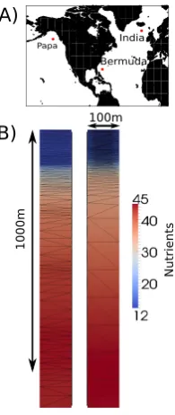
In order to examine a wide range of ocean conditions, three ocean stations (Fig. 1) were chosen to test the performance of mesh adaptivity in conjunction with ocean biogeochemistry models. These were Ocean Weather Station Papa, Ocean Weather Station India and the Bermuda Atlantic Time-series. These stations show very different mixed-layer and biologi-cal behaviours and so test a model’s ability to accurately sim-ulate a range of physical and biological behaviours. Whilst Papa is ideal for carrying out 1-D studies due to the lack of significant horizontal advection (Denman and Miyake, 1973; Gaspar et al., 1990; Burchard and Bolding, 2001), India and Bermuda both experience significant horizontal advection. Previous attempts to model Bermuda in one dimension have resorted to ad hoc “fixes” (Anderson and Pondaven, 2003; Weber et al., 2007) in order to simulate the physical and bio-logical behaviour here. However, the aims of these previous studies were to understand the processes occurring in more detail. In this study we are concerned with how well adap-tive remeshing can replicate the results of a fixed-mesh sim-ulation whilst minimising the number of elements used. We therefore do not expect a perfect match to observed data for these two stations, but the simulations must replicate the gen-eral observed behaviour at all three stations. In addition, we do not necessarily expect model skill to increase when using adaptive remeshing. We are instead examining the numerical response of the model. Without numerical confidence in the model, altering biological parameters to tune the model may “lead to misconceptions in the interpretation of ecosystem dynamics” (Oschlies and Garçon, 1999).
1
0
0
0
m
100m Papa
Bermuda India A)
B)
Nu
tr
ie
n
[image:4.595.119.217.61.293.2]ts
Fig. 1. Map of station locations (A) and 2-D view of the model domain at showing two different meshes produced by the adaptivity algorithm (B).
results from the adaptive mesh simulation. Finally, two ex-periments are described in which the mesh is adapted to con-centrate resolution not only in critical regions such as at the MLD, but also to track sinking detritus at Station Papa to well below the mixed layer depth and the subsurface chlorophyll maximum at Bermuda, which occurs below the mixed layer. The paper then assesses the merits of the adaptive algorithm presented and draws some conclusions.
2 Methods
Here, the non-hydrostatic Boussinesq equation system is considered in the context of Fluidity (Ford et al., 2004; Pain et al., 2005; Piggott et al., 2008b), a highly flexible finite ele-ment/control volume modelling framework which allows for the numerical solution of the following set of equations:
∂u
∂t +u· ∇u+fk×u=
− ∇
p
ρ0
− ρ
ρ0
gk+ ∇ ·(ν∇u) , (1)
∇ ·u=0, (2)
∂T
∂t +u· ∇T = ∇ ·(κT∇T ) , (3)
∂S
∂t +
u· ∇S= ∇ ·(κS∇S) , (4)
ρ≡ρ(T , S), (5)
whereuis the 3-D velocity vector,t represents time, p is
the pressure,gis the acceleration due to gravity acting in the
k=(0,0,1)T direction,T is temperature andSis salinity.ρ
is the density which is given in terms of an equation of state function with temperature and salinity as input arguments, andρ0is a constant background value for density. ν is the
tensor of kinematic viscosities andκT,κS are the thermal
and saline diffusivity tensors respectively.f is the Coriolis parameter which in this work is assumed constant. We also assume, for simplicity, a Cartesian coordinate system with k pointing in the direction of gravity.
The above equations were discretised on an unstruc-tured mesh of tetrahedral elements using the finite-element method. The form of the discretisation is determined by the order of the polynomials used for the different solution vari-ables and whether or not they are continuous or discontin-uous across element faces. A constant time step of 360 s is used with Crank–Nicolson temporal discretisation.
Here, we use a linear continuous Galerkin method for ve-locity and pressure, with a control volume formulation used for all tracer fields, including turbulence and biological trac-ers. Discontinuous linear Galerkin discretisations have also been tested and work successfully. For further details see Pig-gott et al. (2008b, 2009).
2.1 Boundary conditions
The domain used is quasi-1-D, 100 m square in the horizontal with depths of either 1000 m for Station Papa and Bermuda, or 2000 m for Station India. This ensures that the maximum MLD is well above the lower boundary at all stations. The lateral boundaries have a Dirichlet condition applied to the velocity such that the vertical component is zero. The top and bottom surfaces also have this condition applied. Boundary conditions for the turbulent quantities are as described in Hill et al. (2012) and are Neumann conditions for both turbulent equations. The top surface cell is subjected to heat, momen-tum and salinity fluxes. These are derived via the Large and Yeager (2004) bulk formulae, with atmospheric data supplied from ERA40 (Uppala et al., 2005). Both Station Papa and Station India use atmospheric forcing from 1970 onwards as this is when most observation data from those stations are available. Bermuda uses atmospheric forcing from 1980 on-wards, again as most observational data was available during this period. Briefly, the three surface kinematic fluxes cal-culated – heat,hwθi; salt,hwsi; and momentum,hwui and
hwvi – can be related to the surface fluxes of heatQ, the freshwaterF and the momentumτ=(τu, τv)via
hwθi =Q ρCp−
1
(6)
hwsi =Fρ−1S0
(7)
(hwui,hwvi)=τρ−1=(τu, τv) ρ−1, (8)
where ρ is the ocean density, Cp is the heat capacity
applied as upper-surface Neumann boundary conditions on the appropriate fields.
2.2 Biogeochemical model
The model used here is a six-component model similar to the globally applicable model of Popova et al. (2006). Heuristi-cally, the model consists of nutrients (ammonium and nitrate) which are fixed by phytoplankton in the presence of sun-light (photosynthetic active radiation – PAR). Phytoplankton shading is included, reducing the amount of PAR down the water column. Zooplankton grazes on phytoplankton and de-tritus partially recycling them back into inorganic nutrients and partially converting into detritus. Phytoplankton and zoo-plankton mortality also produce detritus which is gradually converted back to nutrients as it sinks through the water col-umn.
Nutrients (ammonium and nitrate), detritus, phytoplank-ton and zooplankphytoplank-ton are solved prognostically, whilst chloro-phyll is a diagnostic variable, derived from phytoplankton. Initial conditions for phytoplankton, detritus and zooplank-ton concentrations were the same for all stations and are 0.1 mmol m−3above 100 m and 0.005 below 100 m. Ammo-nia was set to an initial value of 0.01 mmol m−3. Nitrate pro-files were taken from Kleypas and Doney (2001) for Station Papa and Bermuda and Popova et al. (2006) for station India. For more details of this model see Appendix A1, which in-cludes all parameters used. Note the parameters were tuned to give a good fit to all stations presented here, but were not altered between any model runs.
2.3 Vertical turbulence model
The generic length scale (GLS) turbulence parameterisation simulates vertical turbulence at a finer than that of the mesh. As the GLS model is a RANS parameterisation there is no dependency on the mesh resolution, provided the advective model simulates no turbulent processes, so is ideal for adap-tive ocean-scale problems. GLS has the additional advantage that it can be set up to behave as a number of classical turbu-lence models:k–ǫ,k–kl,k–ω, and an additional model based on Umlauf and Burchard (2003), the gen model. The GLS model has been implemented within Fluidity and shown to work well with adaptive remeshing (Hill et al., 2012). Here, we use it ink–ǫmode as detailed in Hill et al. (2012), which is a two-equation model. The first equation deals with the turbulent kinetic energy,k:
∂k
∂t +ui
∂k
∂xi =
∂ ∂z
ν
M
σk
∂k ∂z
+P+B−ǫ, (9)
whereσk is the turbulence Schmidt number for k, andP
andB represent production by shear and buoyancy which
are defined as
P = −u′w′∂u
∂z−v′w′
∂v
∂z =νMM
2
M2=
∂u
∂z 2
+
∂v
∂z 2
, (10)
B= −g
ρ0
ρ′w′= −νHN2
N2= −g
ρ0
∂ρ
∂z. (11)
Here,Nis the buoyancy frequency,νMis the kinematic eddy
viscosity andνH is the kinematic eddy diffusivity, given by:
νM=√klSM+νM0, νH =√klSH+νH0. (12)
νH0 is the background diffusivity (set to 1×10⁻⁶m2s−1),νM0
is the background viscosity (1×10⁻⁶m2s−1),SM andSH
are often referred to as stability functions,kis the turbulent kinetic energy, andlis a length scale. When using GLS the values ofνM andνH become the vertical components of the
tensorsνandκT in Eqs. (1) and (3) respectively. Other tracer
fields, such as salinity use the same diffusivity as tempera-ture, i.e.κT =κS.
There is also the option to add an extra term to account for additional oceanic physics, such an internal waves break-ing. This is based on the NEMO ocean model (Madec, 2008) and takes a user-defined percentage of the surfacekand dis-tributes it down-depth using an exponential profile:
k(z)=k0(z)+αksurexp(−z/ lk), (13)
wherekis the new turbulent kinetic energy value at depthz,
k0is the original turbulent kinetic energy,ksuris the surface turbulent kinetic energy,αis a constant for the amount (per-centage) of surface turbulent kinetic energy to transfer down the column, andlkis a length scale (m) over which this decay occurs. In this work,α=0.05 andlk=30.
The second equation gives the dissipationǫ, which is de-scribed by
∂ǫ
∂t +
ui ∂ǫ
∂xi =
∂ ∂z
νM
σǫ ∂ǫ ∂z
+ǫ
k(c1P+c3B−c2ǫ), (14)
wherec1,c2,c3 andσǫ are constants with values given by
Hill et al. (2012).
The MLD can be defined in a number of ways. Here, we use two definitions: (1) wherek <1×10⁻⁵m2s−2and (2) where density is 0.125 kg m−3less than surface density (i.e. atz=0). We use the second when comparing to observa-tional data and the first for determining weighting of thek
field when using adaptivity (see next section).
2.4 Dynamic adaptive mesh optimisation
of the mesh in order to minimise an optimisation functional (Pain et al., 2001; Piggott et al., 2005, 2008b). We use the in-terpolation error which is often a reasonable indication of the error due to spatial discretisation in finite-element problems (Pichelina et al., 2000). In Fluidity, mesh adaptivity aims to increase resolution in regions of the domain with large curva-tures of given fields and decrease resolution elsewhere. This approach allows good representation of the small-scale dy-namics and sharp gradients without the need for high spatial resolution throughout the entire domain (Piggott et al., 2005). The mesh is adapted through a series of local topological and geometrical operations as described by Pain et al. (2001). In this work we adapt in the vertical direction only. A single column of mesh vertices is first adapted. This column is then replicated to the other three columns, which are then joined to form a quasi-1-D column of tetrahedra. The location of the vertices is constructed such that all elements in that first 1-D column have unit edge length when measured with respect to a given adaptivity metric,M.
In Fluidity a relatively simple adaptivity metricMis em-ployed. For chosen fieldsfi, adaptivity metricsMi are
de-fined by
Mi =det|Hi|−
1 2p+n |Hi|
εi
, (15)
whereεi is a user-defined weight corresponding to the field under consideration and|Hi|is the Hessian matrix (second-order derivatives) for that field where the absolute values of its eigenvectors have been taken,p∈Zandnis the dimen-sion of the space (Loseille and Alauzet, 2011). The Hes-sian matrix contains information about both the magnitude and direction of the curvature of a field and hence can be used to guide generation of anisotropic elements. The final adaptivity metric used,M, is formed from a superposition of the adaptivity metrics for individual fields:M=S
iMi(Pain
et al., 2001). In the work presented here we tested values of
pof 2 and∞as both have been used in previous work, but
p=2 has shown superior results in resolving both weak and strong curvatures simultaneously within the same simulation (Loseille and Alauzet, 2011; Hiester et al., 2011) and is used in all simulations presented.εmay be varied spatially and temporally, but neither is utilised here. In general, for a given solution field, decreasingεwill lead to greater refinement of the mesh and increasingεwill lead to more coarsening. At this point the adaptivity metric is also modified to take into account bounds upon the maximum and minimum element size, maximum allowable aspect ratio, edge length grada-tion, and number of elements. For more details see Pain et al. (2001); Piggott et al. (2005, 2008b); Hiester et al. (2011) and references therein.
The mesh is adapted at run time and the frequency with which it adapts can also be specified. Here, we specify an adapt frequency of 5 h. After an adapt the solution fields must be interpolated from the pre- to post-adapt meshes. Two methods are available: “linear-interpolation” and “bounded
Galerkin-projection” (Farrell et al., 2009). All prognostic fields are interpolated, along with any diagnostic fields as required. Three different interpolation methods were tested in this work: linear interpolation, which is bounded but non-conservative; Galerkin projection, which is conservative and can be made bounded at the expense of a minimal amount of diffusion (Farrell et al., 2009); and a mixture of the two, in which Galerkin projection was used for biological trac-ers, and linear interpolation was used for physical quantities. It is anticipated that conservation of the integral of biologi-cal quantities is crucial to obtaining a satisfactory solution, but that the physical quantities – velocity, temperature and salinity – only require linear interpolation (Hill et al., 2012). As linear interpolation is less computationally demanding than Galerkin projection, further savings in computational cost over and above those obtained through those obtained through the use of adaptivity can be gained using linear in-terpolation where it is adequate.
The adaptivity metric used to alter the mesh is crucial to obtaining an optimal simulation (Hiester et al., 2011). Here, we test four different adaptivity metric formulations which govern element sizes: PAR, Bio, Bio and Phys, and Phys. These use the photosynthetic active radiation only (PAR), biological fields and photosynthetic active radiation (Bio), physical fields only (Phys) or a combination (Bio and Phys). The same adaptivity metrics are used for all three test stations as we are attempting to provide an adaptivity metric formu-lation that works well in a variety of ocean settings and to avoid “tweaking” of the adaptivity metric for a particular lo-cation. The physical fields used are the density and velocity, and the biological fields used are the nutrients and PAR. De-tails of the fields used and the weighting of each field are given in Table 1. It is important to note that Fluidity allows a great deal of flexibility in choosing the adaptivity metric, un-like in the previous studies described above. Here, we investi-gate how the choice of which fields (physical and biological) are included in the adaptivity metric affects a simulation. We do not investigate the effects of changing the user-defined weights ε; they are chosen to give a reasonable result and may not be optimal. For the purposes of this paperεbeing sub-optimal is not critical. The weights were chosen based on a preliminary parameter study and give a good compro-mise between good results and minimal element numbers.
Table 1. Weighting of fields used for each metric used in this study. A “–” indicates that this field was not used in the metric construction. See Eq. (15).
Metric Nutrient (ε) (mmol m−3) PAR (ε) (W m−2) Velocity (ε) (m s−1) Density (ε) (kg m−3)
Bio 10.0 0.1 – –
Phys – – (0.1, 0.1, 10.0) 0.01
Bio and Phys 10.0 – (0.1, 0.1, 10.0) 0.01
PAR – 0.1 – –
hence phytoplankton high, may not be at the surface; this is the case in Bermuda where there is a significant subsur-face chlorophyll maximum. By resolving the nutrient fluxes closely we aim to also then resolve the other biological trac-ers as a consequence. In contrast, Station Papa shows only weakly varying surface nutrient changes. However, the up-ward flux of nutrients can lead to erroneous timings of the spring bloom. Therefore, the base of the MLD shows a sub-stantial vertical nutrient change and hence adding resolution here should minimise spurious vertical numerical diffusivity. PAR is important only in the top 100 m of the domain and varies daily and hence adding this field to the adaptivity met-ric will add extra resolution during daylight hours down to the bottom of the photic zone.
To examine the effect of adaptive remeshing on biogeo-chemical models we perform a number of experiments. For each station we run fixed mesh simulations at different res-olutions to examine the effects of vertical mesh resolution on the biogeochemistry. We qualitatively compare the results from the highest fixed-mesh resolution to available observa-tions at each station. We then perform experiments varying the adaptivity metric at each station and evaluate the results compared to the highest resolution fixed-mesh simulation us-ing the root mean square error of a number of fields to quan-titatively evaluate the performance. Finally, we perform two specific examples tracking other biological tracers to demon-strate possible uses for the adaptive remeshing technology.
3 Model evaluation
We first examine a single fixed-mesh case for each station, comparing them to available observational data from Kleypas and Doney (2001) and Popova et al. (2006), before showing that the simulated response depends on the model’s vertical resolution.
Station Papa in the Northwest Pacific is an ideal testing station for a 1-D simulation. There is little horizontal advec-tion, and as such, Papa has been used to assess numerical models (Denman and Miyake, 1973; Burchard and Bolding, 2001; Hill et al., 2012). Fluidity has also been previously shown to work well at replicating the expected physics with adaptive meshes here (Hill et al., 2012). Papa’s distinguish-ing feature is that nutrients are not limited and hence sur-face nutrients exhibit only a small seasonal variation. Sursur-face
0 200 400 600 800 1000
Day −200 −150 −100 −50 0 U M L d e p th (m )
0 200 400 600 800 1000
Day 0.0
0.5 1 .0 1 .5 2 .0 2 .5 3.0 3.5 4.0
S u rf a ce C h lo ro p h yl l (m m o l/ m 3)
0 200 400 600 800 1000
Day 0 200 400 600 800 1000 1200 1400 1600 In te g ra te d p ri m a ry p ro d u ct io n (m g C /m 2/d a y)
0 200 400 600 800 1000
Day 0 5 10 15 20 25 S u rf a ce N u tr ie n ts (m m o l/ m 3) Obs. Model
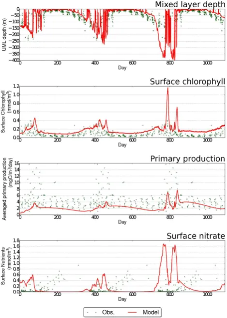
Fig. 2. Summary of simulated physical and biological behaviour at Station Papa for a uniform (2.5 m), non-adaptive simulation. From top to bottom, panels show MLD, surface chlorophyll, integrated primary productivity and surface nutrients. Where available, mea-sured data are shown as green squares. Meamea-sured data are plotted against day of year due to lack of data for some quantities.
[image:7.595.310.546.185.513.2]Fig. 3. Summary of simulated physical and biological behaviour at Bermuda for a uniform (2.5 m), non-adaptive simulation. From top to bottom, panels show MLD, surface chlorophyll, averaged pri-mary productivity and surface nutrients. Where available, measured data are shown as green squares. Measured data are plotted against day of year due to lack of data for some quantities.
agreement to observed data, as does the integrated primary production (note: this is integrated over the mixed layer).
The model result at Bermuda, unlike Papa, shows some differences to the measured data (Fig. 3). The surface nutrient shows the observed nutrient-limited behaviour, but the limit-ing of nutrients occurs too early in the year. The third win-ter (days 700–900) shows a marked deepening of the mixed layer. This is due to surface forcing particular to that year, and longer simulations (not shown) show a return to the more normal behaviour seen in years one and two. Surface chloro-phyll values lie on the upper limit of observed data, with a small peak in the spring. The primary production (note: aver-aged over MLD) is around a factor of two too low. However, given that we are simulating an isolated 1-D column, without any horizontal transport of quantities in or out of the domain, we believe this is a reasonable result. There is a substantial subsurface chlorophyll maximum (Fig. 4) as has been shown in measured observation and it is of similar magnitude to that
Fig. 4. Time–depth plot of chlorophyll at Bermuda, showing the clear subsurface chlorophyll maxima.
obtained in previous modelling studies (e.g. Anderson and Pondaven, 2003).
Unlike for the previous stations there is a lack of MLD data for Station India. However, the model again gives a suf-ficiently good match to available data, although with larger discrepancies compared to other stations (Fig. 5). The spring bloom (as shown by the surface chlorophyll) happens around 30 days early, with a peak that is perhaps a factor of four too high. Similarly, the integrated primary production (note: in-tegrated over the mixed layer) shows a peak of around 2–3 times the observed value at the same time. However, the val-ues during the rest of the year lie around the lower limit of observed data. Surface nutrients show reasonable agreement with the timing of the spring decrease, but the level is perhaps a factor of two too high during the summer months.
3.1 Resolution dependence
For all stations we have run the simulations on a number of fixed meshes, varying the vertical resolution between 20 m and 2.5 m. We use the highest resolution (2.5 m) fixed-mesh simulation as “truth” when assessing the performance of the adaptive mesh simulations. In addition, we use qualitative comparisons to observational data at each station to ensure that the model performs as expected, given the lack of hori-zontal dynamics.
A standard root mean square (rms) error was used to assess model performance. The rms error is calculated as
ǫrms=
v u u u t
n P
i=1
(xi−yi)2
n , (16)
wherexi is the quantity being assessed in the high-resolution
simulation andyi is the value of the quantity produced by
[image:8.595.310.547.63.172.2]Fig. 5. Summary of simulated physical and biological behaviour at Station India for a uniform (2.5 m), non-adaptive simulation. From top to bottom, panels show MLD, surface chlorophyll, integrated primary productivity and surface nutrients. Where available, mea-sured data are shown as green squares. Meamea-sured data are plotted against day of year due to lack of data for some quantities.
nutrients,ǫPfor primary productivity,ǫCfor chlorophyll and
ǫZfor zooplankton. Here, the L2normis defined as
L2norm=
v u u u t
n Z
0
|S|2dV , (17)
whereV is the volume of the domain andSis the scalar field in question.
Figures 6–8 show a single year (year 2 of the 3-year sim-ulation to allow for model spin-up) for each station. For Sta-tion Papa (Fig. 6) there is a noticeable difference in MLD be-haviour with higher resolutions showing deeper winter mix-ing. This in turn affects the upward mixing of nutrients, which show a marked jump when resolution is refined from 10 to 5 m. Both 5 and 2.5 m resolutions show broadly sim-ilar patterns. The difference in upward mixing of nutrients then affects the primary productivity, and surface chlorophyll shows a difference in peak surface chlorophyll of around
400 450 500 550 600 650 700
Day
−140
−120
−100
−80
−60
−40
−20
0
UML
dep
th
(m)
400 450 500 550 600 650 700
Day 0.1
0.2 0.3 0.4 0.5 0.6 0.7
Sur
face
Chl
oro
ph
yll
(mm
ol/
m
3)
400 450 500 550 600 650 700
Day 0
100 200 300 400 500 600
Int
eg
rate
d
pr
imar
y
pro
duct
ion
(mg
C/m
2/da
y)
400 450 500 550 600 650 700
Day 10.0
10.5 11.0 11.5 12.0 12.5 13.0
Sur
face
Nut
rien
ts
(mm
ol/
m
3)
2.5m 5m
10m 20m
Mixed layer depth
Surface chlorophyll
Primary production
Surface nitrate
Fig. 6. Summary of simulated physical and biological behaviour at Station Papa using uniform meshes at a number of resolutions. From top to bottom, panels show MLD, surface chlorophyll, integrated primary productivity and surface nutrients.
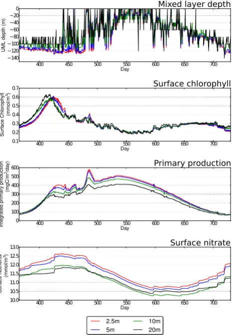
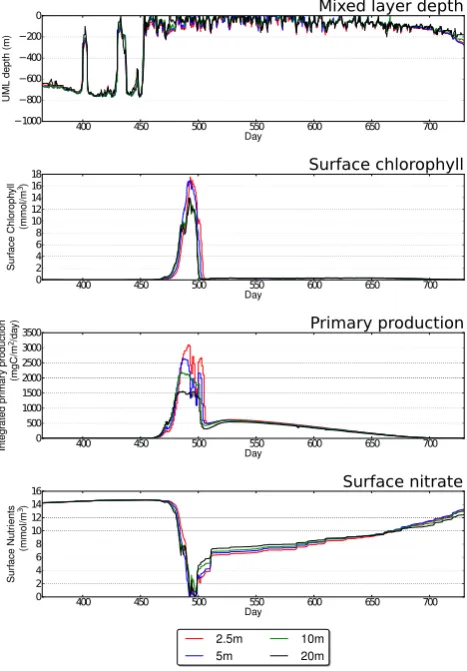
20 days. Bermuda shows a similar pattern (Fig. 7) with creased resolution producing higher peak nutrients due to in-creased upmixing, which in turn leads to inin-creased surface chlorophyll. Finally, Station India (Fig. 8) shows a marked increase in primary productivity within the MLD, which is doubled when resolution is refined from 20 to 2.5 m. The surface nutrient data show little difference with resolution, so a sensible interpretation is that this is due to the slight increase in summer MLD depths with increased resolution. It is therefore clear that all stations show a response to ver-tical resolution which is the result of a complex interaction between the mixing caused by the vertical turbulence model and the biological sources and sinks.
[image:9.595.313.547.63.399.2]Table 2. The rms error,ǫ, of fixed-mesh simulations compared to the simulation with 2.5 m vertical resolution at Station Papa.ǫis shown for MLD, and the L2normof nutrient, primary productivity, chlorophyll and zooplankton. See Fig. 6 also.
Res (m) ǫMLD(m) ǫN(mmol m−3) ǫP(mmol m−3) ǫC(mmol m−3) ǫZ(mmol m−3) No. elements
5 m 5.244 0.119 0.098 0.0095 0.0045 1200
10 m 10.640 0.506 0.342 0.0445 0.0169 600
[image:10.595.84.511.208.264.2]20 m 16.521 0.421 0.628 0.0486 0.0283 300
Table 3. The rms error,ǫ, of fixed-mesh simulations compared to the simulation with 2.5 m vertical resolution at Bermuda.ǫis shown for MLD, and the L2normof nutrient, primary productivity, chlorophyll and zooplankton. See Fig. 7 also.
Res (m) ǫMLD(m) ǫN(mmol m−3) ǫP(mmol m−3) ǫC(mmol m−3) ǫZ(mmol m−3) No. elements
5 m 7.079 0.408 0.140 0.0129 0.0113 1200
10 m 12.630 0.402 0.149 0.0160 0.0236 600
20 m 18.710 0.397 0.226 0.0285 0.0410 300
400 450 500 550 600 650 700
Day −300 −250 −200 −150 −100 −50 0 UML dep th (m)
400 450 500 550 600 650 700
Day 0.05
0.10 0.15 0.20 0.25 0.30 0.35 0.40 0.45
Sur face Chl oro ph yll (mm ol/ m 3)
400 450 500 550 600 650 700
Day 1.0
1.5 2.0 2.5 3.0 3.5 4.0 4.5
A ver age d pr imar y pro duct ion (mg C/m 3/da y)
400 450 500 550 600 650 700
Day 0.0
0.1 0.2 0.3 0.4 0.5 0.6 0.7
Sur face Nut rien ts (mm ol/ m 3) 2.5m 5m 10m 20m
Mixed layer depth
Surface chlorophyll
Primary production
Surface nitrate
Fig. 7. Summary of simulated physical and biological behaviour at Bermuda using uniform meshes at a number of resolutions. From top to bottom, panels show MLD, surface chlorophyll, MLD aver-aged primary productivity and surface nutrients.
400 450 500 550 600 650 700
Day −1000 −800 −600 −400 −200 0 UML dep th (m)
400 450 500 550 600 650 700
Day 0 2 4 6 8 10 12 14 16 18 Sur face Chl oro ph yll (mm ol/ m 3)
400 450 500 550 600 650 700
Day 0 500 1000 1500 2000 2500 3000 3500 Int eg rate d pr imar y pro duct ion (mg C/m 2/da y)
400 450 500 550 600 650 700
Day 0 2 4 6 8 10 12 14 16 Sur face Nut rien ts (mm ol/ m 3) 2.5m 5m 10m 20m
Mixed layer depth
Surface chlorophyll
Primary production
Surface nitrate
[image:10.595.312.546.299.635.2] [image:10.595.50.285.304.634.2]Table 4. The rms error,ǫ, of fixed-mesh simulations compared to the simulation with 2.5 m vertical resolution at Station India.ǫis shown for MLD, and the L2normof nutrient, primary productivity, chlorophyll and zooplankton. See Fig. 8 also.
Res (m) ǫMLD(m) ǫN(mmol m−3) ǫP(mmol m−3) ǫC(mmol m−3) ǫZ(mmol m−3) No. elements
5 m 137.03 1.04 303.258 1.538 0.222 2400
10 m 138.18 1.21 357.834 1.770 0.247 1200
20 m 142.71 1.50 455.565 1.992 0.264 600
to nearly 120 m when resolution is increased from 20 to 2.5 m. Bermuda shows a decrease of both winter and summer subsurface chlorophyll maxima with increasing resolution. These vertical profiles show that the model is numerically stable, producing adequate results at even low resolution, but that vertical resolution does affect the profile simulated.
The response to resolution can be examined more quan-titatively using a simple convergence test. Although conver-gence is non-trivial for nonlinear dynamics (Hill et al., 2012), a decrease in error should be seen with increasing vertical resolution. For all stations there is clear convergence (a de-crease in error) for the MLD (Tables 2–4). Ideally, for the set-up described previously, this should be at least first-order convergence. Both Bermuda and Station Papa show this be-haviour but Station India does not (though there is still a de-crease in error with increasing resolution). However, for most variables there is a decrease in the error measure compared to the highest resolution simulations at each station.
The surface nutrients error stays approximately constant at both Bermuda and Station India (Tables 3 and 4). Despite these exceptions there is a clear dependence on resolution, with higher resolutions generally matching the highest reso-lution simulation with higher accuracy. At Papa, all biologi-cal quantities bar nutrients show a general convergence in er-ror as resolution is increased (Table 2). The erer-ror at 10 m ver-tical resolution appears to be double that expected, but there is a convergence in error from 10 to 5 m. Bermuda shows clear first-order convergence of MLDs and zooplankton; and less certain convergence of chlorophyll (Table 3). Surface nu-trient error appears to be constant, as does primary produc-tivity (average over the MLD). Finally, Station India shows a general convergence with increasing resolution for all bio-logical quantities, though not at first order (Table 4).
From these results we can see that there is a general de-crease in error to the highest resolution run with increasing resolution. Therefore, using vertical adaptivity should allow a minimisation in the number of elements within the compu-tational mesh whilst ensuring that error does not increase to an unreasonable level.
4 Adaptivity
We have carried out the same simulations as above using an adaptive mesh guided by a variety of different adaptivity met-rics and, in addition, we have tested different interpolation
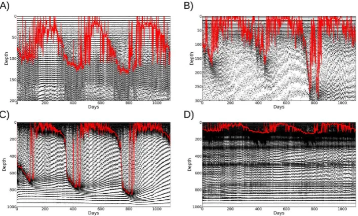
[image:11.595.336.516.144.590.2]Fig. 10. Representation of the meshes obtained via adaptivity for all stations using the bio and phys metric. A dot is placed on each vertex in the mesh and this is repeated for each output time. Clustering of vertices therefore indicate higher resolution. Station Papa (A) shows reduced resolution under the mixed layer during summer, but high resolution persists for some distance below the mixed layer. Bermuda (B) shows substantial reduction of resolution below the mixed layer, but with the minimum resolution being maintained during the summer in the upper layers. Similarly, India (C) tracks the MLD, with decreased resolution within the mixed layer, whilst maintaining good resolution in the upper portion of the water column. Gradients in density mean that high-resolution zones are maintained at Station Papa (D) at up to 800 m depth.
methods at Station Papa. For simplicity, simulations at the three test station used the same adaptivity settings. Adaptiv-ity was performed every 5 h. This allows changes in ocean surface forcing (which has a temporal frequency of 6 h) to be captured, along with diurnal fluctuations. Over a 3-year simulation a total of 5256 adapts are thus performed. This is a large number and therefore any additional numerical diffu-sivity or noise derived from adapting the mesh will be evident in the final simulation results when compared to the fixed-mesh simulations. The minimum and maximum edge lengths permitted are set to 5 and 50 m respectively. We therefore hope to find that the adaptive simulations are equivalent to the 5 m fixed resolution simulations, but use substantially fewer elements.
The adaptive algorithm was performed on a single vertical column of mesh vertices and the position of these were repli-cated to the other three columns. In this way we obtained a layered mesh, with vertical resolution of the layers varying according to the chosen adaptivity metric and the simulated state at the time of the adapt. Apart from the adaptive mesh, the simulations were completely identical to the fixed-mesh simulations.
The meshes produced by the adaptive algorithm showed broadly similar features between different adaptivity metrics for each particular site (Fig. 10). Comparing those produced by the adaptivity metric using both the biological and physi-cal fields shows the mesh tracking the behaviour of the MLD.
In addition, high resolution is maintained in the photic layer, but reduces with the mixed layer when the MLD increases substantially.
4.1 Effect of interpolation method
[image:12.595.121.475.62.275.2]Table 5. The rms error,ǫ, of adaptive mesh simulations compared to the simulation with 2.5 m vertical resolution at Station Papa.ǫis shown for MLD, and the L2normof nutrient, primary productivity, chlorophyll and zooplankton. See Fig. 6 also.
Res (m) ǫMLD(m) ǫN(mmol m−3) ǫP(mmol m−3) ǫC(mmol m−3) ǫZ(mmol m−3) No. elements (Mean, min, max)
5 m 5.244 0.119 0.0986 0.0095 0.0045 1200
Bio and Phys 4.769 0.053 0.385 0.0038 0.0020 458.5, 372, 558
Bio Only 14.211 0.589 0.529 0.0426 0.0300 386.1, 336, 450
Phys Only 4.837 0.070 0.398 0.0034 0.0021 310.1, 240, 408
PAR 23.324 2.664 0.592 0.0790 0.0330 612.2, 532, 660
0 200 400 600 800 1000
Day −200 −150 −100 −50 0 U M L d e p th (m )
0 200 400 600 800 1000
Day 0 1 2 3 4 5 6 7 S u rf a ce C h lo ro p h yl l (m m o l/ m 3)
0 200 400 600 800 1000
Day 0.0
0.2 0
.4 0.6 0.8 1
.0 1.2 1.4 1 .6 S u rf a ce Z o o p la n kt o n (m m o l/ m 3)
0 200 400 600 800 1000
Day 0 500 1000 1500 2000 In te g ra te d p ri m a ry p ro d u ct io n (m g C /m 2/d a y)
0 200 400 600 800 1000
Day 0 5 10 15 20 25 S u rf a ce N u tr ie n ts (m m o l/ m 3) Obs. Fixed Galerkin Linear Mixed
Fig. 11. Summary of simulation results from Station Papa compar-ing the fixed high-resolution (2.5 m) simulation with adaptive sim-ulation using different interpolation methods between meshes. Lin-ear and mixed perform poorly, inducing extra vertical diffusivity, compared to Galerkin projection. Panels and data are the same as in Fig. 6.
However, here we have added the additional term to simu-late internal wave breaking (Eq. 13) and the adaptivity met-ric in Hill et al. (2012) was tuned to Station Papa only, with a lower minimum edge length. It is also worth noting that the temperature and salinity fields showed little or no difference between the fixed and adaptive simulations as was shown in Hill et al. (2012); it is the biological tracers that highlight un-desired behaviour, i.e. upward fluxing of tracers, of the adap-tive runs. Galerkin projection is therefore used for all subse-quent adaptive simulations.
400 450 500 550 600 650 700
Day −200 −150 −100 −50 0 UML dep th (m)
400 450 500 550 600 650 700
Day 0.1
0.2 0.3 0.4 0.5 0.6 0.7
Sur face Chl oro ph yll (mm ol/ m 3)
400 450 500 550 600 650 700
Day 0 100 200 300 400 500 600 Int eg rate d pr imar y pro duct ion (mg C/m 2/da y)
400 450 500 550 600 650 700
Day 10.0
10.5 11.0 11.5 12.0 12.5 13.0
Sur face Nut rien ts (mm ol/ m 3) Fixed Bio and Phys
Bio only Phys Only
Mixed layer depth
Surface chlorophyll
Primary production
[image:13.595.56.282.105.502.2]Surface nitrate
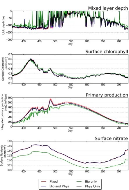
Fig. 12. Summary of results comparing different adaptivity metrics against measured data and the high-resolution (2.5 m) fixed-mesh simulation for Station Papa.
4.2 Station Papa
[image:13.595.317.539.182.510.2]Table 6. The rms error,ǫ, of adaptive mesh simulations compared to the simulation with 2.5 m vertical resolution at Bermuda.ǫis shown for MLD, and the L2normof nutrient, primary productivity, chlorophyll and zooplankton. Note that the PAR and Bio only simulations failed
and recorded no result. See Fig. 7 also.
Res (m) ǫMLD(m) ǫN(mmol m−3) ǫP(mmol m−3) ǫC(mmol m−3) ǫZ(mmol m−3) No. elements (Mean, min, max)
5 m 7.079 0.408 0.140 0.0129 0.0113 1200
Bio and Phys 7.309 0.407 0.598 0.0084 0.0096 310.3, 264, 444
[image:14.595.55.542.212.292.2]Phys Only 8.432 0.408 0.615 0.0076 0.0082 228.3, 174, 436
Table 7. The rms error,ǫ, of adaptive mesh simulations compared to the simulation with 2.5 m vertical resolution at Station India.ǫis shown for MLD, and the L2normof nutrient, primary productivity, chlorophyll and zooplankton. See Fig. 8 also.
Res (m) ǫMLD(m) ǫN(mmol m−3) ǫP(mmol m−3) ǫC(mmol m−3) ǫZ(mmol m−3) No. elements (Mean, min, max)
5 m 137.03 1.04 303.258 1.538 0.222 2400
Bio and Phys 141.98 1.12 356.798 1.668 0.236 287.74, 150.0, 456.0
Bio Only 112.72 1.12 324.777 1.052 0.097 220.63, 120.0, 360.0
Phys Only 141.30 1.08 344.102 1.683 0.237 249.53, 150.0, 414.0
PAR 131.84 1.17 677.312 1.920 0.245 120.00, 120.0, 121.0
the adaptivity metric is not adequate at this location as the values of the rms errors, ǫ, for all tracers are substantially larger, apart from primary productivity, which has already been identified as potentially problematic in use as an assess-ment of performance.
4.3 Bermuda
Not all adaptive simulations were effective at Bermuda. Us-ing either PAR or biology only to form the adaptivity met-ric results in simulations failing with a solver error soon af-ter the first or second adapt. This is attributed to insufficient mesh resolution to ensure stability for the GLS turbulence parameterisations. Unlike Station Papa, the MLD is well be-low the photic zone in the initial stages of the simulation. However, both simulations using either physics only or biol-ogy and physics performed well. Both gave similar results, quantitatively (Table 6) and qualitatively (Fig. 13). The two adaptivity metrics also gave lower values ofǫCandǫZ, but, as with Station Papa, these values should interpreted with some caution.
4.4 Station India
All adaptive simulations produced good results at Station In-dia when compared to the high-resolution fixed-mesh reso-lution regardless of adaptivity metric used (Table 7, Fig. 14). Minor differences in the timing of the spring bloom occurred with the biology-only adaptivity metric occurring some 25 days later than the fixed-mesh simulation. The biology-only adaptivity metric also showed an increase in the number of shoaling excursions in the spring. These did not occur when using other adaptivity metrics or in the fixed-mesh simula-tions. There are also minor differences in the magnitude of
the integrated primary productivity, but these variations are much lower than those observed when changing resolution in the fixed-mesh simulations (Figs. 8).
4.5 Summary of adaptive results
Adaptive remeshing can clearly be successfully applied at the three ocean stations successfully using a variety of adap-tivity metrics. Some adapadap-tivity metric/station combinations perform better than others. As well as reproducing the sur-face values (i.e. at depthz=0) and the MLD the adaptive simulations also reproduce the vertical profiles of biologi-cal parameters (see Fig. 15 for chlorophyll and compare to Fig. 9).
The effect of adaptivity is clearly seen in the meshes pro-duced by the simulations (Fig. 10). All stations show much higher resolution around the MLD, as expected, with de-creased resolution when the MLD is deep (for example at Station India). The meshes contain far fewer elements than the high-resolution fixed-mesh simulations and are therefore more computationally efficient.
400 450 500 550 600 650 700 Day −300 −250 −200 −150 −100 −50 0 UML dep th (m)
400 450 500 550 600 650 700
Day
0.05 0.10 0.15 0.20 0.25 0.30 0.35 0.40 0.45
Sur face Chl oro ph yll (mm ol/ m 3)
400 450 500 550 600 650 700
Day 1 2 3 4 5 6 A ver age d pr imar y pro duct ion (mg C/m 3/da y)
400 450 500 550 600 650 700
Day
0.0 0.1 0.2 0.3 0.4 0.5 0.6 0.7
Sur face Nut rien ts (mm ol/ m 3) Fixed Bio and Phys
Phys Only
Mixed layer depth
Surface chlorophyll
Primary production
[image:15.595.51.285.61.401.2]Surface nitrate
Fig. 13. Summary of results comparing different adaptivity metrics against measured data and the high-resolution (2.5 m) fixed-mesh simulation at Bermuda. Note that the simulations using PAR and biology only failed after only a few adapts.
sensible choices (Hill et al., 2012). Accounting for physical behaviour in the adaptivity metric appears to be sufficient for a successful simulation of biological behaviour. However, if the physical properties are well simulated then the biologi-cal processes do not necessarily also need including in the adaptivity metric in order to achieve a reasonable output.
5 Specific adaptive examples
One of the primary advantages of the approach outlined above is that the adaptivity metric used to calculate the mesh edge length can be composed of any simulated or diagnosed fields. We show the potential of that method here by simulat-ing Bermuda with a adaptivity metric focussimulat-ing on chloro-phyll, and Station Papa concentrating on sinking detritus. These simulations show how the mesh is able to adapt to the particulars of the simulation, tracking transient behaviour but with a lower computational overhead than a high-resolution fixed-mesh simulation.
400 450 500 550 600 650 700
Day −1200 −1000 −800 −600 −400 −200 0 UML dep th (m)
400 450 500 550 600 650 700
Day 0 2 4 6 8 10 12 14 16 18 Sur face Chl oro ph yll (mm ol/ m 3)
400 450 500 550 600 650 700
Day 0 500 1000 1500 2000 2500 3000 3500 Int eg rate d pr imar y pro duct ion (mg C/m 2/da y)
400 450 500 550 600 650 700
Day 0 2 4 6 8 10 12 14 16 Sur face Nut rien ts (mm ol/ m 3) Fixed Bio and Phys
Bio only Phys Only
Mixed layer depth
Surface chlorophyll
Primary production
[image:15.595.313.545.64.398.2]Surface nitrate
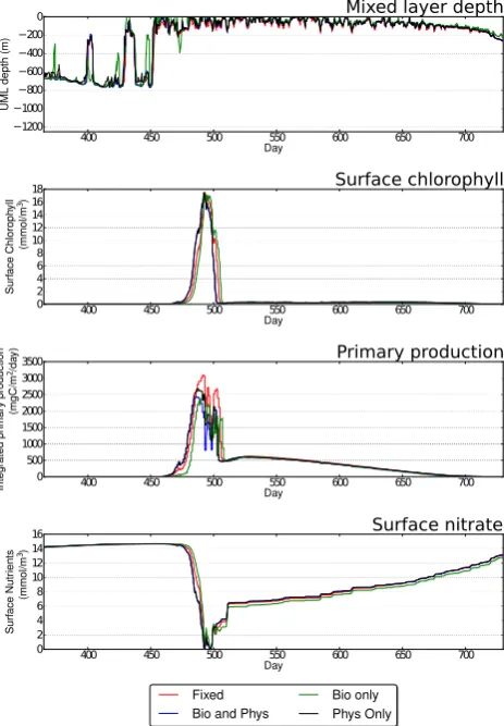
Fig. 14. Summary of results comparing different adaptivity metrics against measured data and the high-resolution (2.5 m) fixed-mesh simulation for Station India.
Fig. 15. Vertical profiles of chlorophyll at (A) Station Papa, (B) Bermuda and (C) Station India over the top 150 m, 150 m and 200 m respectively comparing the performance of different adaptiv-ity metrics. The left-hand column shows the profile in summer (day 182) and the right-hand column shows the profile in winter (day 365). Note that all metrics, bar biology only, show similar results.
A similar result is seen at Bermuda where chlorophyll is added to the adaptivity metric. Here, we see that the subsur-face chlorophyll maximum is maintained correctly (Fig. 18), whereas in the previous adaptive simulation the simulated value is lower around day 130 than for the fixed-mesh sim-ulation. This is not the case when chlorophyll is added to the adaptivity metric. The simulation using a typical ocean model vertical resolution shows a lower chlorophyll peak (day 100) and a slightly reduced subsurface chlorophyll maximum throughout the summer compared to the high-resolution simulation. The effect of adding chlorophyll to the adaptivity metric can be seen in the resulting mesh (Fig. 17).
For both simulations there is, of course, an increase in the number of elements used compared to the original adap-tive simulations, but the average number of elements is still much lower than the high-resolution fixed-mesh simulation, and accordingly, the run times are much lower. The Bermuda simulation used an average of 437 elements (576 maximum, 301 minimum). Compared to a fixed mesh of uniform reso-lution 2.5 m (2400 elements) this is a fivefold reduction in el-ements on average. The simulation based on a typical ocean model vertical resolution uses 216 elements at the coast of reduced resolution of the chlorophyll maximum. Similarly, simulating detritus at Station Papa used an average of 726 el-ements (507 minimum, 1120 maximum), compared to 2400 elements used in the 2.5 m fixed mesh simulation – a three-fold reduction. The simulation using typical ocean model vertical resolution uses 216 elements (as at Bermuda) and is clearly incapable of accurately resolving sinking detritus.
6 Conclusions
This work has shown that the Fluidity model can success-fully replicate expected biogeochemical behaviour at three key ocean stations. Both fixed and adaptive mesh simulations show very similar behaviour, but adaptive remeshing requires careful consideration of the adaptivity metric used. The phys-ical quantities must be included in this adaptivity metric, and if the physical properties are well simulated then biological tracers do not necessarily need including in the adaptivity metric for reasonable output. This is consistent with a num-ber of other studies where physical processes are the domi-nate control of ocean biogeochemical models (Berline et al., 2007). It is important to note that we have not shown an increase in model skill with either increasing resolution of when using adaptive meshes. We have, however, attempted to demonstrate numerical convergence of the biological model with increasing resolution.
A) B)
De
p
th
(
m
)
0
750 375
0 Days 365
De
p
th
(
m
)
0
750 375
0 Days 365
De
p
th
(
m
)
0
750 375
0 Days 365
De
p
th
(
m
)
0
750 375
0 Days 365
C) D)
0.075
0.0 0.35
De
tr
itu
s
(
m
m
o
l/
m
3)
0.075
0.0 0.35
De
tr
itu
s
(
m
m
o
l/
m
[image:17.595.131.464.65.249.2]3)
Fig. 16. Time–depth plot of detritus at Station Papa from the original adaptive mesh simulation (A), the adaptive run with detritus included in the metric (B), the high-resolution fixed-mesh simulation (C), and (D) the same simulation using decreasing resolution with increasing depth. Including detritus in the adaptive metric increases the performance of the model at tracking detritus to depth, resolving detail in the timing and level of detrital pulses. Note that (D) smooths those events into a single unresolved event by day 300.
De
p
th
(
m
)
0
400 200
A)
De
p
th
(
m
)
0
400 200
B)
De
p
th
(
m
)
0
750 375
C)
De
p
th
(
m
)
0
750 375
D)
0 365 Days 720 1095 0 365 Days 720 1095 0 365 Days 720 1095 0 365 Days 720 1095
Fig. 17. Comparison of meshes produced by adaptive simulations. (A) Bermuda with the addition of chlorophyll to the adaptivity metric, (B) the original adaptive simulation at Bermuda using velocity, density and nutrients. Similarly, for Station Papa: (C) adaptive simulation with detritus included in the metric and (D) original adaptive simulation
in the vertical for large-scale ocean models (Piggott et al., 2008a) and is similar to the method used by Hofmeister et al. (2010). The work here is therefore compatible with how Flu-idity will simulate global- or regional-scale models, using an unstructured horizontal mesh, with each vertical column then being extruded to the required depth. However, each column contains a different number of nodes in these cases which may induce additional vertical diffusivity due to horizontal gradients in the mesh. More work is required to ascertain if this effect is present in such simulations.
[image:17.595.132.453.330.518.2]A) B)
D) C)
De
p
th
(
m
)
0
250 125
De
p
th
(
m
)
0
250 125
De
p
th
(
m
)
0
250 125
De
p
th
(
m
)
0
250 125
365 Days 720
365 Days 720
365 Days 720
365 Days 720
Di
ff
e
re
n
c
e
0.08
-0.1 0
0.6
0.0 0.3
C
h
l-a
(
m
m
o
l/
m
[image:18.595.130.463.65.253.2]3)
Fig. 18. Difference plots of chlorophyll at Bermuda comparing adaptive simulations (A and B) and a fixed, but varying resolution mesh (C) to the highest resolution (2.5 m) uniform mesh simulation (D). A clear improvement can be made in the subsurface chlorophyll maximum representation by adding chlorophyll to the adaptivity metric. (A) The original adaptive mesh simulation shows larger discrepancies around the subsurface maximum (B). Using fixed variable resolution as in other ocean models shows clear discrepancies in the spring and throughout the summer (C).
need to be constant for each spatial location. Instead, as is shown here, the resolution only needs to be placed at key locations in the vertical. Enabling higher resolution around the MLD and within the upper layers of the ocean is suffi-cient for replicating high-resolution fixed-mesh simulations, hence adaptive remeshing may be advantageous. However, note that we have kept other parameters that may depend on resolution constant, including the biogeochemical model pa-rameters. The turbulence parameterisation is not resolution dependant provided the model does not attempt to resolve the turbulent scales included in the parameterisation. This is the case here. For the stations simulated here , using the normal
ocean model vertical resolution where resolution decreases with depth is sufficient to obtain a reasonable solution. How-ever, mesh adaptivity also has another powerful feature: ad-ditions to the adaptivity metric of other fields allows for the tracking of transient features and of other fields, such as de-tritus or chlorophyll. This is a powerful tool in tracking fea-tures of interest whilst minimising the number of elements in the computational mesh.
Appendix A
Biology model
As stated in the main body of the text, the biogeochemical model used in this report was based on that of Popova et al. (2006). Note, however, that the equations here are continu-ous for all depths, which was not true in Popova et al. (2006) where different source terms where used below the photic zone. The model parameters have also been fitted to match the data at all three test sites. The six components of the model are: nutrients (ammonium and nitrate), phytoplankton, chlorophyll, zooplankton and detritus.
A1 Biological source terms
The source terms for phytoplankton (P), chlorophyll (Chl), zooplankton (Z), nitrate (N), ammonium (A) and detritus (D) respectively are given by the following expressions:
SP=PJ (QN+QA)−GP−DeP, (A1)
SChl=(RP·J·(QN+QA)·P
+(−GP−DeP))·θ/ζ ), (A2)
SZ=δ·(βP·GP+βD·GD)−DeZ, (A3)
SN= −J·P·QN+DeA, (A4)
SA= −J·P·QA+DeD+(1−δ)·(βP·GP
+βD·GD)+(1−γ )·DeZ−DeA, (A5)
SD= −DeD+DeP+γ·DeZ
+(1−βP)·GP−βD·GD. (A6)
The terms in these equations are given in Table A1.
Note that unlike the model of Popova et al. (2006) we use a continuous model, with no change of equations (bar one exception) above or below the photic zone. For our purposes, the photic zone is defined as 100 m water depth. First we calculateθ:
θ=Chl
Pζ . (A7)
However, at low light levels, Chl might be zero, there-fore we take the limit thatθ→ζ at low levels (1×10⁻⁷) of chlorophyll or phytoplankton.
We then calculateα:
α=αcθ (A8)
using the PAR available at each vertex of the mesh the light-limited phytoplankton growth rate,J, is then calculated:
J=p vαIn
v2+α2+I2
n
. (A9)
This can be used to calculate the limiting factors on nitrate and ammonium:
QN=
N exp−9A
KN+N
, (A10)
QA=
A
KA+A
(A11)
From these the diagnostic field, primary production (XP), can be calculated:
XP=J (QN+QA)P. (A12)
The chlorophyll growth scaling factor is given by
RP=QNQA
θ
m θ
v
p
v2
+α2
+I2
n !
. (A13)
The zooplankton grazing terms are now calculated:
GP=
gpPP2Z
ǫ+ pPP2+pDD2
, (A14)
GD=
gpDD2·Z
ǫ+ pPP2+pDD2. (A15)
Finally, the four death rates and re-mineralisation rates are calculated:
DeP= µpP 2 P+kp +
λbio·P, (A16)
DeZ= µzZ 3 Z+kz+
λbio·Z, (A17)
DeD=µDD+λbio·P+λbio·Z, (A18)
DeA=λAA where z <100. (A19)
A2 Photosynthetically active radiation (PAR)
The photosynthetically active radiation, or PAR is calculated by
PAR=(Awater+APP)I, (A20) whereAwaterandAPare the absorption rates of photosynthet-ically active radiation by water and phytoplankton respec-tively.
A3 Detritus sinking velocity
Table A1. Symbols used to describe the six-component NPZD model. Typical values are provided for externally set parameters.
Symbol Meaning Typical value Equation
α initial slope ofP–Icurve in (W m−2)−1day−1 Eq. (A8)
αc Chl-aspecific initial slope ofP−Icurve 2 gC gChl−1(W m−2)−1day−1
βP, βD assimilation coefficients of zooplankton 0.75
DeD rate of breakdown of detritus to ammonium Eq. (A18)
DeP rate of phytoplankton natural mortality Eq. (A16)
DeZ rate of zooplankton natural mortality Eq. (A17)
DeA ammonium nitrification rate Eq. (A19)
δ excretion parameter 0.7
ǫ grazing parameter relating capture of prey items to prey density 0.4
GP rate of zooplankton grazing on phytoplankton Eq. (A14)
GD rate of zooplankton grazing on detritus Eq. (A15)
g zooplankton maximum growth rate 1.3 day−1
γ fraction of zooplankton mortality going to detritus 0.5
I0 photosynthetically active radiation (PAR) immediately below
surface of water. Assumed to be 0.43 of the surface radiation
J light-limited phytoplankton growth rate in day−1 Eq. (A9)
kA half-saturation constant for ammonium uptake 0.5 mmol m−3
kN half-saturation constant for nitrate uptake 0.5 mmol m−3
kP half-saturation constant for phytoplankton mortality 1 mmol m−3
kZ half-saturation constant for zooplankton mortality 3 mmol m−3
kw light attenuation due to water 0.04 m−1
kc light attenuation due to phytoplankton 0.03 m2mmol−1
λbio rate of the phytoplankton and zooplankton transfer into detritus 0.05 day−1
λA nitrification rate 0.03 day−1
µP phytoplankton mortality rate 0.05 day−1
µZ zooplankton mortality rate 0.2 day−1
µD detritus reference mineralisation rate 0.05 day−1
9 strength of ammonium inhibition of nitrate uptake 2.9 (mmol m−3)−1
pP relative grazing preference for phytoplankton 0.75
pD relative grazing preference for detritus 0.25
QN non-dimensional nitrate limiting factor Eq. (A10)
QA non-dimensional ammonium limiting factor Eq. (A11)
RP Chl growth scaling factor Eq. (A13)
v Maximum phytoplankton growth rate 1 day−1
wg detritus sinking velocity 10 m day−1
z depth
θ Chl to carbon ratio in mgChl mgC−1
θm maximum Chl to carbon ratio 0.05 mg Chl mgC−1
Acknowledgements. All authors were funded by NERC under
grants NE/F00270X/1 and NE/F004184/1. The authors would like to acknowledge the use of the Imperial College London HPC service to perform some of the simulations presented here. The authors would like to thank the two anonymous reviewers for their helpful comments and suggestions.
Edited by: E. J. M. Delhez
References
Anderson, T. R. and Pondaven, P.: Non-redfield carbon and nitro-gen cycling in the Sargasso Sea: pelagic imbalances and ex-port flux, Deep Sea Res.-Pt. I, 50, 573–591, doi:10.1016/S0967-0637(03)00034-7, 2003.
Berline, L., Brankart, J.-M., Brasseur, P., Ourmières, Y., and Verron, J.: Improving the physics of a coupled physical– biogeochemical model of the North Atlantic through data as-similation: Impact on the ecosystem, J. Mar. Syst., 64, 153–172, doi:10.1016/j.jmarsys.2006.03.007, 2007.
Burchard, H. and Beckers, J.-M.: Non-uniform adaptive verti-cal grids in one-dimensional numeriverti-cal ocean models, Ocean Model., 6, 51–81, doi:10.1016/S1463-5003(02)00060-4, 2004.
Burchard, H. and Bolding, K.: Comparative Analysis of
Four Second-Moment Turbulence Closure Models for the Oceanic Mixed Layer, J. Phys. Oceanogr., 31, 1943–1968, doi:10.1175/1520-0485(2001)031<1943:CAOFSM>2.0.CO;2, 2001.
Denman, K. and Miyake, M.: Upper Layer Modification at Ocean Station Papa: Observations and Simulation, J. Phys. Oceanogr., 3, 185–196, 1973.
Farrell, P., Piggott, M., Pain, C., Gorman, G., and Wilson, C.: Con-servative interpolation between unstructured meshes via super-mesh construction, Comput. Method. Appl. M., 198, 2632–2642, doi:10.1016/j.cma.2009.03.004, 2009.
Ford, R., Pain, C. C., Piggott, M. D., Goddard, A. J. H., de Oliveira, C. R. E., and Umpleby, A. P.: A Nonhydrostatic Finite-Element Model for Three-Dimensional Stratified Oceanic Flows. Part I: Model Formulation, Mon. Weather Rev., 132, 2816–2831, doi:10.1175/MWR2824.1, 2004.
Friedrichs, M. A., Hood, R. R., and Wiggert, J. D.: Ecosystem model complexity versus physical forcing: Quantification of their relative impact with assimilated Arabian Sea data, Deep Sea Res.-Pt. II, 53, 576–600, doi:10.1016/j.dsr2.2006.01.026, 2006. Gaspar, P., Grégoris, Y., Lefevre, J.-M., and Goris, Y. G. R. I.:
A Simple Eddy Kinetic Energy Model for Simulations of the Oceanic Vertical Mixing: Tests at Station Papa and Long-Term Upper Ocean Study Site, J. Geophys. Res., 95, 16179–16193, doi:10.1029/JC095iC09p16179, 1990.
Hanert, E., Deleersnijder, E., and Legat, V.: An adaptive finite element water column model using the Mellor-Yamada level 2.5 turbulence closure scheme, Ocean Model., 12, 205–223, doi:10.1016/j.ocemod.2005.05.003, 2006.
Hiester, H., Piggott, M., and Allison, P.: The impact of mesh adaptivity on the gravity current front speed in a two-dimensional lock-exchange, Ocean Model., 38, 1–21, doi:10.1016/j.ocemod.2011.01.003, 2011.
Hill, J., Piggott, M., Ham, D., Popova, E., and Srokosz, M.: On the performance of a generic length scale turbulence model within
an adaptive finite element ocean model, Ocean Model., 56, 1–15, doi:10.1016/j.ocemod.2012.07.003, 2012.
Hofmeister, R., Burchard, H., and Beckers, J.-M.: Non-uniform adaptive vertical grids for 3D numerical ocean models, Ocean Model., 33, 70–86, doi:10.1016/j.ocemod.2009.12.003, 2010. Ji, R., Davis, C., Chen, C., and Beardsley, R.: Influence of
local and external processes on the annual nitrogen cy-cle and primary productivity on Georges Bank: A 3-D biological–physical modeling study, J. Mar. Syst., 73, 31–47, doi:10.1016/j.jmarsys.2007.08.002, 2008.
Kettle, H. and Merchant, C. J.: Modeling ocean primary production: Sensitivity to spectral resolution of attenuation and absorption of light, Prog. Oceanogr., 78, 135–146, doi:10.1016/j.pocean.2008.04.002, 2008.
Khangaonkar, T., Sackmann, B., Long, W., Mohamedali, T., and Roberts, M.: Simulation of annual biogeochemical cycles of nu-trient balance, phytoplankton bloom(s), and DO in Puget Sound using an unstructured grid model, Ocean Dynam., 62, 1353– 1379, doi:10.1007/s10236-012-0562-4, 2012.
Kleypas, J. A. and Doney, S. C.: Nutrients, Chlorophyll, Primary Production and related Biogeochemical Properties in the Ocean Mixed Layer, Tech. Rep. TN-447+STR, NCAR, available at: http://rda.ucar.edu/datasets/ds259.0/ (last access: 8 May 2014), 2001.
Large, W. G. and Yeager, S. G.: Diurnal to decadal global forcing for ocean and sea-ice models: The data sets and flux climatologies, Tech. Rep. Technical Report TN-460+STR, NCAR, 2004. Lévy, M., Iovino, D., Resplandy, L., Klein, P., Madec, G.,
Tréguier, A.-M., Masson, S., and Takahashi, K.: Large-scale impacts of submesoLarge-scale dynamics on phytoplankton: Local and remote effects, Ocean Model., 43-44, 77–93, doi:10.1016/j.ocemod.2011.12.003, 2012.
Loseille, A. and Alauzet, F.: Continuous Mesh Framework Part II: Validations and Applications, SIAM J. Numer. Anal., 49, 61–86, doi:10.1137/10078654X, 2011.
Luo, L., Wang, J., Schwab, D. J., Vanderploeg, H., Leshke-vich, G., Bai, X., Hu, H., and Wang, D.: Simulating the 1998 spring bloom in Lake Michigan using a coupled physical-biological model, J. Geophys. Res.-Oceans, 117, C10011, doi:10.1029/2012JC008216, 2012.
Madec, G.: NEMO ocean engine, Note du Pole de modélisation, Institut Pierre-Simon Laplace (IPSL), France, No. 27 ISSN No 1288-1619, 2008.
McGillicuddy, D. J., Anderson, L. A., Doney, S. C., and Mal-trud, M. E.: Eddy-driven sources and sinks of nutrients
in the upper ocean: Results from a 0.1◦ resolution model
of the North Atlantic, Global Biogeochem. Cy., 17, 1035, doi:10.1029/2002GB001987, 2003.
Menendez, A. N., Badano, N. D., Lopolito, M. F., and Re, M.: Water quality assessment for a coastal zone through numerical modeling, J. Appl. Water Eng. Res., 1, 8–16, doi:10.1080/23249676.2013.827892, 2013.
Oschlies, A.: Can eddies make ocean deserts bloom?, Global Bio-geochem. Cy., 16, 1106, doi:10.1029/2001GB001830, 2002. Oschlies, A. and Garçon, V.: An eddy-permitting coupled