This is a repository copy of The impact of using social media data in crime rate calculations: shifting hot spots and changing spatial patterns.
White Rose Research Online URL for this paper: http://eprints.whiterose.ac.uk/80371/
Version: Accepted Version
Article:
Malleson, N and Andresen, MA (2015) The impact of using social media data in crime rate calculations: shifting hot spots and changing spatial patterns. Cartography and Geographic Information Science, 42 (2). ISSN 1523-0406
https://doi.org/10.1080/15230406.2014.905756
[email protected] https://eprints.whiterose.ac.uk/ Reuse
Unless indicated otherwise, fulltext items are protected by copyright with all rights reserved. The copyright exception in section 29 of the Copyright, Designs and Patents Act 1988 allows the making of a single copy solely for the purpose of non-commercial research or private study within the limits of fair dealing. The publisher or other rights-holder may allow further reproduction and re-use of this version - refer to the White Rose Research Online record for this item. Where records identify the publisher as the copyright holder, users can verify any specific terms of use on the publisher’s website.
Takedown
If you consider content in White Rose Research Online to be in breach of UK law, please notify us by
This is an AuthorÕs Accepted Manuscript of an article published in Cartography and Geographical Information Society (10 Apr 2014), available online:
http://www.tandfonline.com/10.1080/15230406.2014.905756
The impact of using social media data in crime rate calculations:
shifting hot spots and changing spatial patterns
Nick Malleson and Martin Andresen
Abstract
The crime rate is a statistic used to summarise the risk of criminal events. However, research has shown that choosing the appropriate denominator is non trivial. Different crime types exhibit different spatial opportunities and so does the population at risk. The residential population is the most commonly used population at risk, but is unlikely to be suitable for crimes that involve mobile populations. In this paper, we use
Ôcrowd-sourcedÕ data in Leeds, England to measure the population at risk, considering violent crime. These new data sources have the potential to represent mobile populations at higher spatial and temporal resolutions than other available data. Through the use of two local spatial statistics (Getis-Ord GI* and the Geographical Analysis Machine) and visualization we show that when the volume of social media messages, as opposed to the residential population, is used as a proxy for the population at risk criminal event hot spots shift spatially. Specifically, the results indicate a significant shift in the city center, eliminating its hot spot. Consequently, if crime reduction/prevention efforts are based on resident population based crime rates, such efforts may not only be ineffective in
reducing criminal event risk, but be a waste of public resources.
Introduction
The spatially-referenced crime rate is a statistic often used to represent the risk of
criminal events. Spatially-referenced crime rates help to reveal clusters of crime in space and/or time based on an underlying population at risk. However, the choice of an
appropriate population at risk is non trivial. Different crime types have different spatial opportunity sets that necessitate the separate analyses. Similarly, the population at risk varies for different crime rates and should be given the same consideration. As stated by Boggs, Ôa valid rate ... should form a probability statement, and therefore should be based on the risk or target group appropriate for each specific crime categoryÕ (Boggs 1965, 900). Despite this importance, most research uses the residential (census) population as the population at risk, primarily because of data availability and constraints in terms of time and money. Although it has been claimed that it matters little which poulation at risk is used in the analysis (Cohen et al. 1985), recent research suggests that the residential population is unsuitable as a measure of population at risk for crimes that involve mobile victims such as assaults (Boivin 2013), robbery (Zhang et al. 2012) and automotive theft, burglary, and violent crime (Andresen 2006, 2011).
1. Are crime hotspots stable under the application of different population-at-risk measures?
2. Which areas have the highest crime rates when using both residential (census) and mobile (social media) population at risk data?
Related Work
The Population at Risk in Crime Analysis
resolution is relatively poor for spatial crime analysis (approximately the size of a census tract) because recent research has shown that analysing crime at scales greater than the street segment may hide important lower-level patterns (Andresen and Malleson 2011); and 2) the ambient population estimate is a yearly average, such that no account is taken for seasonal variations or the differences in population counts at different times of day. In an attempt to allieviate some of these problems, this paper will use data contributed by individuals to social media services to estimate ambient population at risks.
Social Media Data for Mobile Populations
In recent years, the emergence of vast new administrative and commercial data sources, coupled with warnings about a ÒcrisisÓ in an empirical sociology that continued to rely entirely on traditional small studies (Savage and Burrows, 2007), has spurred some research to engage with new forms of Ôcrowd sourcedÕ data to gain insight into social processes. These data, that have commonly been contributed informally by citizens, rather than as part of a formal survey, are becoming ubiquitous and will undoubtedly have a dramatic impact future social science research. With respect to population dynamics in particular, traditional large-volume social science data lack information regarding where people are throughout the day, instead representing the night time
And in the context of this paper, such data may prove to be useful for spatial crime analysis.
The number of sources for such data is increasing with the more widely used being Twitter, mobile device data from service providers, public transport usage, Foursquare, Flickr, and Facebook. Research in the United States has found that that two-thirds of online adults (66 percent) use social media platforms (Smith, 2011) and that 26 percent of American Internet users aged 18-29 have been found to use Twitter (Smith and Brenner, 2012). Data from these sources are also volumnous. For example, there were supposedly over 100 million active Twitter accounts in 2011 (Twitter, 2011) and 270,000 tweets per minute produced worldwide in 2012 (TechCrunch, 2012).
Social media data have recently been used for a wide variety of different purposes Ð a full review of applications would be an extensive undertaking (and one that would be outdated before it is published). However, examples of the application of social media data to the study of social phenomena are more limitted. Examples include research into the fear of missing out (Przybylski al., 2013), wellbeing (Hong et al., 2012) and
happiness over time (Bliss et al., 2012). Others make some limitted use of the data, but still resort to traditional sampling methods (see, for example, Fischer and Reuber, 2011; Wohn et al., 2013). The most relevant research for this project are those that have started to make use of the geographical locations of social media messages, although given the novelty of utilising these data sources examples are still rare. Relevant research includes: the mathematical analysis of human mobility patterns (Cheng et al. 2011); the
earthquakes (Crooks et al. 2013) and other geographical patterns (Stefanidis et al., 2013) in social media data; and the use of Google search trends to estimate the locations of new outbreaks of influenza (Ginsberg et al., 2009). However, we are unaware of any research that uses social media data to better understand the risk of criminal victimization.
Despite their relatively widespread (and increasing) use, these data sources do have limitations. Such data are inherently ÔmessyÕ in the sense that they are not gathered using a systematic and statistically guided methodology such as a census. As a result, data structures may be poorly defined, missing data are commonplace, and there are no systematic ÔcorrectionsÕ for these issues because these data are still so new to research. Additionally, because of these issues we must also be concerned with generalizability. For example, Li et al. (2013), as part of a special issue on mapping cyberspace and social media, found that higher socioeconomic status groups are overrepresented in Twitter and Flickr. This is not inherently problematic, particularly in the current context of measuring populations at risk, because these higher socioeconomic groups may be representative of the underlying population distribution, on average. The main difficulty arrises in testing such a hypothesis. However, even if only a portion of the actual population is being captured, the bias inherent in residential populations for measuring the population at risk may be reduced.
Study area and data overview
Leeds and the census data
business and retailing district with a high concentration of shops, businesses and
entertainment facilities. This district attracts large volumes of people from within Leeds, Bradford, Manchester, and a number of smaller towns/villages on the outskirts of the city. Such areas have long been known to have high levels of crime because they attract large volumes of people (Schmid 1960a, 1960b) and the centre of Leeds is no exception; the district has high volumes of violent crime relative to surrounding areas. Related to the alternative population at risk literature in spatial crime analysis, relatively few people live in the city center, upwardly biasing any representations of criminal event risk using the resident population.
In order to measure the residential population, we have used the number of people residing in each Output Area (OA) at the time of the 2011 UK census. The OA geography is the smallest area for which census statistics are released. Each OA has a recommended size of 125 households, but can vary based on natural boundaries and the presence (or absence) or high-density housing.
Crime data
The criminal event data used in the analyses below include all individual occurrences of violent crime in 2011 within the Leeds Local Authority District (N=10,625) that were reported to the police. These data were obtained from the police.uk service
murder (Flatley 2013b). A drawback with these data is that it is not possible to disaggregate the crime type further (for example it might be advantageous to analyse robbery and assault separately as research has shown that the spatial patterns of spcific crime types can be rather different (Andresen and Linning, 2012)). For privacy reasons, the police.uk service aggregates individual crime points to the nearest Ôanonymous map pointÕ that can be the center of a street segment, a public place or a commercial building. These points are defined with catchment areas that have at least eight unique postal addresses, approximately the size of a city block. Although such an aggregation process inevitably induces some spatial inaccuracy, the impact is unlikely to influence any results because the direction in which the criminal event points are moved is random in the aggregate. Also, because Leeds is a rather densely populated city, it unlikely that any individual criminal event points will be displaced far from their actual location.
Additionally, we could disaggregate the data temporally, an obvious application of social media data because of the availability of when messages are posted. We do not undertake such an analysis, and leave it for future research, because the first comparison in the spatial crime analysis context is with how crime data are mapped in the majority of research, an aggregated year.
Social Media data
will explore the possibility of including a varity of sources (e.g. Stefanidis et al. 2013) although as Twitter is by far the most widely used service it is not clear that the incorporation of additional services is necessary in this application. Because we are interested in the spatial dimension of criminal victimization risk, only messages with associated GPS coordinates have been included. Such data are commonly generated using mobile devices by users who have explicitly opted to publish their present location. A manual inspection of the data revealed many high volume accounts were not individual people (examples include weather forecasts, car advertisements, etc.). After deleting these data, the number of messages in our sample was almost 2 million, N=1,955,655. In addition to the location, each individual message contains information regarding the user account, the text itself, and the time of the message. These additional fields allow for the creation of a temporally dynamic population at risk or an exploration of the
characteristics of the individuals who make up the general population. Both of these factors could lead to even more accurate risk estimates, although this is not under investigation here and is a direction for future research.
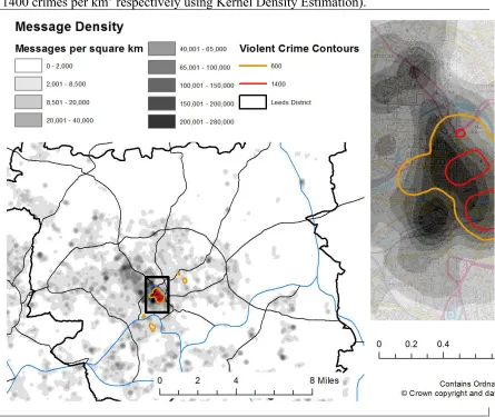
The density of the messages overlaid with violent crime hot spots is shown in Figure 1.1 As would be expected, message densities are greatest in urban areas and particularly in the city centre. This is precisely what would be expected, based on what we know regarding the ambient population. Consequently, as hypothesized above, despite not having a representative sample of individuals based on socioeconomic status, based
1The density per unit area is used in order to facilitate subsequent comparisons in the
on local knowledge of the study area, these data may appear to be representative of where people actually are. And, of great interest for the current paper, the largest densities of messages appear to coincide with the greatest densities of violent crimeÑthis is not the case with the resident population.
Figure 1. Kernel density of social media messages and violent crime contours. The contours depict the areas with the largest volume of violent crime (densities of 600 and 1400 crimes per km2 respectively using Kernel Density Estimation).
Methods and Results
will apply two complementary statistics that can be used to identify clusters in spatial data. Both search for clusters of crime by comparing volumes in individual areas to their surrounding neighbours and to global averages. They are known as Local Indicators of Spatial Association (LISA) and offer the advantage of testing for statistical significance
of apparent clustersÑsee Anselin (1995) for a discussion of LISA statistics. Both statistics will be used to search for statistically significant crime hotspots using census data and social media data as the populations at risk.
Statistic 1: Getis-Ord GI*
The first statistic to be applied is the Getis-Ord GI* (Getis and Ord 1992; Ord and Getis 1995). This is used here because its definition closely matches that of a Ôhot spotÕÑlocal area averages that are significantly greater than global averages (Chainey and Ratcliffe 2005)Ñand has hence become popular within spatial criminological research. We use first order queenÕs contiguity in the analyses below.
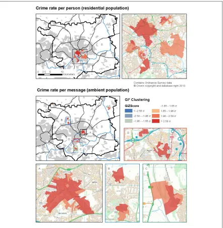
Figure 2 maps the GI* indices for the two violent crime rates. Output areas with insignificant p values (0.05 < p < 0.95) are not shown, regardless of their Z value. The distribution of significant GI* scores proves to be instructive. When considering the residential violent crime rate, there is a statistically significant cluster in the city center as well as in some of the surrounding neighborhoods. The violent crime cluster in the city center is expected, particularly because of the low residential population and large
JamesÕs University Hospital) to the north-east and two small areas in neighborhoods to the south-west. It should be noted, however, that the violent crime cluster surrounding the university hospital may simple be a reporting issues: violent criminal events are coded to occur at this location because this is where they are reported.
A number of violent clusters emerge when using the ambient violent crime rate (see Figure 2 insets A, B, C, D). Curiously, none of the violent crime clusters include the city center area, suggesting the violent crime rate there is not significant when using the ambient population to measure the population at risk. Rather, the violent crime clusters are in diverse neighborhoods with no obvious single explanation for their existence. Each of these neighborhoods may have high violent crime rates given the size of the population at risk. This is clearly a direction for further research.
A drawback with the GI* statistic is that it requires the spatial aggregation of point data into areas (output areas in this case). Therefore it is susceptible to the modifiable areal unit problem (Openshaw 1984). Hence a second statistic is also used that avoids aggregation to the output area geography in order to further assess the differences in the two violent crime rate calculations.
Statistic 2: The Geographical Analysis Machine
!! ! !! !!
!!
(1)
where !! is the total number of observations (crimes), !! is the size of the base
population (number of residents or number of messages) and pi is the size of the base population within search circle i. Then the difference, di, is calculated from the expected number of observations to the actual number of observations, ai, that occur within circle i:
!! ! !! ! !!. (2)
If a larger number of cases are found than would be expected (di > 0), a Poisson test for statistical significance is performed. The test calculates the probability that the number of observed events is the same as the number of expected events (d = 0). If this probability is lower than a set threshold Ð in this case the threshold is 0.0099 Ð then the null hypothesis is rejected and the difference is statistically significant at the specified threshold. In these cases the search circle is stored as a potential cluster. The GAM output is a list of search points and the difference between the expected and actual number events (di) when di is statistically significant.
This algorithm has been chosen to comlement the GI* analysis because, importantly, it minimizes the impact of the modifiable areal unit problem by defining arbitrary search locations on a regular grid and also by varying the search radius for each search point. In this manner, clusters that appear at one resolution can be discarded if they disappear at others. A further advantage of the GAM algorithm is that it will process raw point data directlyÑspatial aggregation is not a prerequisite.
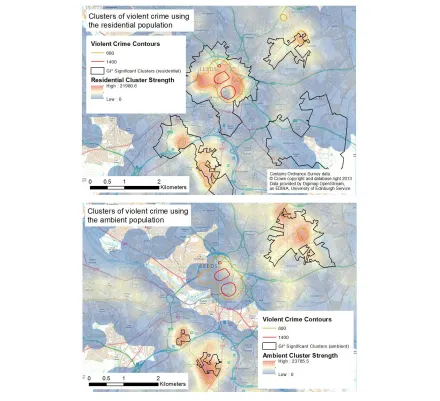
to generate a single density map. The difference between the expected and actual numbers of crimes at each search point (i.e. the output of the algorithm) were used to calculate the density. In this manner, the most dense areas will be those that have a large difference at multiple resolutions. Clusters that are only significant at a small number of search radii will only add marginally to the density of their area. The results are mapped in Figure 3.
The first noteable result is that the GAM outputs are largely in agreement with those of the GI* analysis. Both techniques reveal broadly similar cluster locations regardless of the population at risk used. Considering the number of social media messages, the large volume of violent crime in the city centre is only marginally higher than would be expected given the ambient population. In other words, the risk of violent criminal victimization is not particularly high in the city center. However, the algorithms both identify violent crime clusters in neighborhoods to the north- and south-east regardless of the population at risk used. The consistency with which these areas have been identified as crime ÔhotspotsÕ suggests that they are indicitative of an exceptionally high volume of crime, whereas the city centre hotspot is more likely to be an artefact of the size of the ambient population.
Discussion and conclusions
In this analysis, we have shown that different spatial patterns of crime rates emerge when using two different population at risk measures: the residential population (measured by the 2011 UK census) and the ambient population (measured by counting the number of messages posted to the Twitter social media service). One may say that such a conclusion is an obvious one, but it is important to recognize that the use of an ambient population measure is justified by theory as well as previous empirical research despite the
the high volume of violent criminal events, there is not a statistically significant elevation in risk of violent criminal victimizaton when considering a theoretically-informed
population at risk. No such conclusion would have been reached with the residential population.
Additionally, there are a small number of neighborhoods very close to the city center that exhibit significantly high violent crime rates when considering both populations at risk, regardless of the clustering method. There is no obvious reason for such high rates of violent crime. These neighborhoods score rather high on the deprivation scale, with two of the neiborhorhoods scoring 114 and 128 highest in England out of a total of 32,482 neighborhoods. Given that deprivation is a highly complex phenomenon, considering a multitude of social factors, it may be the case that this plays some role through (a lack of) oppportunity in terms of legitimate activities for residents social tension that leads to violence. This is clearly an area of future research interest as well.
Though we have had some interesting, and theoretically expected, results, our analysis is not without its limitations. Most specifically, we must be cautious with the use of Twitter data and making generalizations about general population movements. How well do the spatial locations of social media messages reflect the actual spatial locations of the ambient population, in general? We know that some socioeconomic groups are
media are increasing, the percentage of messages that include accurate geogrpahic information are as low as 1-2 percent (Leetaru et al. 2013; Gelernter and Mushegian 2011). Finally, there is the potential for participation inequality stemming from the differences in the prevalence of social media useage across different social groups. A body of work has explored the impacts of the Ôdigital divideÕ (e.g. Yu, 2006; Fuchs, 2009) and it is possible that the higher crime rates identified in the north-east and south-west neighbourhoods are an artefact of lower Twitter usage in these relatively deprived communities. However, it is not clear how well general trends in digital access are reflected in Twitter usage Ð further research is required to establish whether or not the ambient population in these neighbourhoods is poorly represented by Twitter data. The persistance of the hotspots regardless of the population at risk used here does, however, add strength to the results.
In general, there are potential problems that must be investigated for the appropriate use of crowd sourced data. However, if they can be resolved there is great potential, particularly for spatial crime analysis. For example, Twitter data, or social media data more generally, could be used to estimate particular sub-populations at risk of particular crime types such as young people who visit bars during the evening. Therefore, the population at risk could be tailored according the the most likely victims of a particular crime category to answer the call made by Boggs (1965) almost 50 years ago: Ôthe risk or target group appropriate for each specific crime categoryÕ (Boggs 1965, 900).
potential to describe social phenomena better than well organised small surveys or even national censuses. Mayer-Schonberger and Cukier (2013) share this view:
One of the areas that is being most dramatically shaken up by N=all is the social sciences. They have lost their monopoly of making sense of empirical social data, as big data analysis replaces the highly skilled survey specialists of the past. .. When data are collected passively while people do what they
normally do anyway, the old biases associated with sampling and questionnaires disappear (30).
We are confident that the messy, biased and noisy aspects of big data will soon be reduced for confident use in the social sciences. Though they may not disappear or be at the same low level as with more formal data gathering techniques, these limitations may simply become outweighed by the sheer volume of crowd sourced data and the ways in which it can be utilized. We were able to obtain nearly 2 million individual datum with a minimal setup time and negligible financial cost. Also, with increased use and demand for such data, the providers of social media may very well increase the quality of their data and metadata because they will realize the value of their commodity. We have argued above that its utility is significant for spatial crime analysis.
References
Andresen, M.A., 2006. ÒCrime Measures and the Spatial Analysis of Criminal Activity.Ó
British Journal of Criminology 46 (2): 258Ð285.
Andresen, M.A., 2011. ÒThe Ambient Population and Crime Analysis.Ó Professional Geographer 63 (2): 193Ð212.
Andresen, M.A., and G.W. Jenion. 2010. ÒAmbient Populations and the Calculation of Crime Rates and Risk.Ó Security Journal 23 (2): 114Ð133.
Andresen, M.A., G.W. Jenion, and A.A. Reid. 2012. ÒAn Evaluation of Ambient Population Estimates for Use in Crime Analysis.Ó Crime Mapping: A Journal of Research and Practice 4(1): 7Ð30.
Andresen, M.A., and S.J. Linning 2012. ÒThe (In)appropriateness of Aggregating Across Crime Types.Ó Applied Geography 35 (1-2): 275 - 282.
Andresen, M.A., and N. Malleson. 2011. ÒTesting the Stability of Crime Patterns:
Implications for Theory and Policy.Ó Journal of Research in Crime and Delinquency
48 (1): 58Ð82.
Anselin, L. 1995. ÒLocal Indicators of Spatial Association Ð LISA.Ó Geographical Analysis 27 (2): 93 Ð 115.
Bliss, C. A., I. M. Kloumann, K. D. Harris, C. M. Danforth and P. S. Dodds. 2012. "Twitter Reciprocal Reply Networks Exhibit Assortativity with Respect to Happiness." Journal of Computational Science 3 (5): 388-397.
Boivin, R. 2013. ÒOn the Use of Crime Rates.Ó Canadian Journal of Criminology and Criminal Justice 55 (2): 263Ñ277.
Chainey, S., and J.H. Ratcliffe. 2005. GIS and Crime Mapping. Chichester: John Wiley and Sons.
Cheng, Z., J. Caverlee, K. Lee, and D. Z. Sui. 2011. ÒExploring Millions of Footprints in Location Sharing Services.Ó In Proceedings of the Fifth International AAAI
Conference on Weblogs and Social Media (ICWSM), July 2011, Barcelona, 81Ð88. Menlo Park, CA: AAAI press.
Cohen, L.E., R.L. Kaufman, and M.R. Gottfredson. 1985. ÒRisk-Based Crime Statistics: A Forecasting Comparison for Burglary and Auto Theft. Journal of Criminal Justice
13 (5): 445Ð457.
Corcoran, J.J., I.D. Wilson, and J. Ware. 2003. ÒPredicting the Geo-Temporal Variations of Crime and Disorder. International Journal of Forecasting 19 (4): 623Ð634. Cranshaw, J., R. Schwartz, J. Hong, and N. Sadeh. 2012. ÒThe Livehoods Project:
Utilizing Social Media to Understand the Dynamics of a City.Ó In Proceedings of the Sixth International AAAI Conference on Weblogs and Social Media (ICWSM), May 2012, Dublin, 58 Ð 65. Menlo Park, CA: AAAI press.
Crooks, A., A. Croitoru, A. Stefanidis, and J. Radzikowski. 2013. Ò#Earthquake: Twitter as a Distributed Sensor System.Ó Transactions in GIS 17 (1): 124Ð147.
Fischer, I. and A. R. Reuber. 2011. "Social Interaction via New Social Media: (How) Can Interactions on Twitter Affect Effectual Thinking and Behavior?" Journal of Business Venturing 26 (1): 1-18.
Flatley, J. 2013a. Focus on: Violent Crime and Sexual Offences, 2011/12. London: Office for National Statistics.
Flatley, J. 2013b. Crime in England and Wales, year ending September 2012. London: Office for National Statistics.
Fuchs, C. 2008. The Role of Income Inequality in a Multivariate Cross-National Analysis of the Digital Divide. Social Science Computer Review 27: 41Ð58.
Gelernter, J., and N. Mushegian. 2011. ÒGeo-parsing Messages from Microtext. Geo-parsing Messages from Microtext 15 (6): 753Ð773.
Getis, A., and J.K. Ord. 1992. ÒThe Analysis of Spatial Association by Use of Distance Statistics.Ó Geographical Analysis 24 (3): 189Ð206.
Ginsberg, J., M. H.. Mohebbi, R. S. Patel, L. Brammer, M. S. Smolinski1 and L. Brilliant . 2009. "Detecting Influenza Epidemics Using Search Engine Query Data.", Nature
457: 1012-1014.
Hong, L., A. Ahmed, S. Gurumurthy, A. Smola and T. Kostas. 2012. "Discovering Geographical Topics in the Twitter Stream." Proceedings of the 21st International Conference on World Wide Web, Lyon, France, pp. 769-778.
Li, L., M.F. Goodchild, and B. Xu. (2013). ÒSpatial, Temporal, and Socioeconomic Patterns in the Use of Twitter and Flickr.Ó Cartography and Geographic Information Science 40(2): 61 Ð 77.
Mayer-Schonberger, V., and K. Cukier. 2013. Big Data: A Revolution That Will Transform How We Live, Work and Think. London: John Murray.
Office for National Statistics. 2012. Mid-2012 Population Estimates. [online] Available online: http://www.ons.gov.uk/ons/rel/pop-estimate/population-estimates-for- england-and-wales/mid-2012/mid-2012-population-estimates-for-england-and-wales.html [Accessed 28 November 2013].
Openshaw, S. 1984. The Modifiable Areal Unit Problem. Concepts and Techniques in Modern Geography (CATMOG) Vol. 38. Norwich: Geo Books.
Openshaw, S. 1987. ÒAn Automated Geographical Analysis System.Ó Environment and Planning A 19 (4): 431Ð436.
Openshaw, S., M. Charlton, and A. Craft. 1988. ÒSearching for Leukaemia Clusters Using a Geographical Analysis Machine.Ó Papers in Regional Science 64 (1): 95Ð 106.
Ord, J.K., and A. Getis. 1995. ÒLocal Spatial Autocorrelation Statistics: Distributional Issues and an Application.Ó Geographical Analysis 27 (4): 286-306.
Przybylskia, A. K., K. Murayamab, C. R. DeHaanc, V. Gladwelld. 2013. "'Motivational, Emotional, and Behavioral Correlates of Fear of Missing Out." Computers in Human Behavior 29 (4): 1841Ð1848.
Savage, M., and R. Burrows. 2007. ÒThe Coming Crisis of Empirical Sociology.Ó
Schmid, C.F. 1960a. ÒUrban Crime Areas: Part I.Ó American Sociological Review 25(4): 527 Ð 542.
Schmid, C.F. 1960b. ÒUrban Crime Areas: Part II.Ó American Sociological Review 25(5): 655 Ð 678.
Smith, A. 2011. Why Americans use social media. Technical report, Pew Research Centre Available online: http://www.pewinternet.org/Reports/2011/Why-Americans-Use-Social-Media.aspx [Accessed 28 November 2013].
Smith, A., and J. Brenner. 2012. Twitter Use 2012. Technical report, Pew Research Center Available online: http://pewinternet.org/Reports/2012/Twitter-Use-2012.aspx [Accessed 28 November 2013].
Stefanidis, A., A. Crooks and J. Radzikowski. 2013. ÒHarvesting ambient geospatial information from social media feeds.Ó GeoJournal 78: 1Ð20.
Smith, A., and J. Brenner. 2012. Twitter Use 2012. Technical report, Pew Research Center Available online: http://pewinternet.org/Reports/2012/Twitter-Use-2012.aspx [Accessed 28 November 2013].
TechCrunch (2012). Analyst: Twitter Passed 500M Users In June 2012. Online:
http://techcrunch.com/2012/07/30/analyst-twitter-passed-500m-users-in-june-2012-140m-of-them-in-us-jakarta-biggest-tweeting-city/ [Accessed on 19/1/13].
Twitter (2011) One hundred million voices. Twitter Blog. Online:
https://blog.twitter.com/2011/one-hundred-million-voices [accessed Jan 2014] Wohn, D. Y., N. Ellison, M. L. Khan, R. Fewins-Bliss, R. Gray. 2013. "The Role of
Yu, L. 2006. Understanding information inequality: Making sense of the literature of the information and digital divides. Journal of Librarianship and Information Science
38: 229Ð252.