Link invariants from finite categorical groups

White Rose Research Online URL for this paper:

http://eprints.whiterose.ac.uk/112769/

Version: Accepted Version

Article:

Martins, JF and Picken, R (2015) Link invariants from finite categorical groups. Homology,

Homotopy and Applications, 17 (2). pp. 205-233. ISSN 1532-0073

https://doi.org/10.4310/HHA.2015.v17.n2.a11

This is an author produced version of a paper published in Homology, Homotopy and

Applications. Uploaded in accordance with the publisher's self-archiving policy.

[email protected] https://eprints.whiterose.ac.uk/

Reuse

Items deposited in White Rose Research Online are protected by copyright, with all rights reserved unless indicated otherwise. They may be downloaded and/or printed for private study, or other acts as permitted by national copyright laws. The publisher or other rights holders may allow further reproduction and re-use of the full text version. This is indicated by the licence information on the White Rose Research Online record for the item.

Takedown

If you consider content in White Rose Research Online to be in breach of UK law, please notify us by

Homology, Homotopy and Applications, vol. 16(2), 2014, pp.1–29

LINK INVARIANTS FROM FINITE CATEGORICAL GROUPS

JO ˜AO FARIA MARTINS and ROGER PICKEN

(communicated by Bill Murray)

Abstract

We define an invariant of tangles and framed tangles given a finite crossed module and a pair of functions, called a Rei-demeister pair, satisfying natural properties. We give several examples of Reidemeister pairs derived from racks, quandles, rack and quandle cocycles, and central extensions of groups. We prove that our construction includes all rack and quandle cohomology (framed) link invariants, as well as the Eisermann invariant of knots. We construct a class of Reidemeister pairs which constitute a lifting of the Eisermann invariant, and show through an example that this class is strictly stronger than the Eisermann invariant itself.

1.

Introduction

In knot theory, for a knotK, the fundamental groupπ1(CK) of the knot comple-mentCK, also known as the knot group, is an important invariant, which however depends only on the homotopy type of the complement ofK(for which it is a complete invariant), and therefore, for example, it fails to distinguish between the square knot and the granny knot, which have homotopic, but non-diffeomorphic complements. Nevertheless, a powerful knot invariantIGcan be defined from any finite groupG, by counting the number of morphisms from the knot group intoG. In a recent advance, Eisermann [13] constructed, from any finite group G and any x∈G, an invariant

E(K) that is closely associated to a complete invariant [29], known as the peripheral system, consisting of the knot group π1(CK) and the homotopy classes of a merid-ian m and a longitude l. Eisermann gives examples showing that his invariant is capable of distinguishing mutant knots as well as detecting chiral (non-obversible), non-inversible and non-reversible knots (using the terminology for knot symmetries employed in [13]). Explicitly the Eisermann invariant for a knotK is:

E(K) = X

{f:π1(CK)→G|f(m)=x}

f(l),

and takes values in the group algebraZ_{[G] ofG.}

Received Month Day, Year, revised Month Day, Year; published on Month Day, Year. 2010 Mathematics Subject Classification: 57M25, 57M27 18D10

Key words and phrases: Knot invariant, tangle, peripheral system, quandle, rack, crossed module, categorical group, non-abelian tensor product of groups.

Article available athttp://dx.doi.org/10.4310/HHA.2014.v16.n2.a1

Eisermann’s invariant has in common with many other invariants that it can be calculated by summing over all the different ways of colouring knot diagrams with algebraic data. Another well-known example of such an invariant is the invariant

IG defined above, which can be calculated by counting the number of colourings of the arcs of a diagram with elements of the groupG, subject to certain (Wirtinger) [8] relations at each crossing. Another familiar construction is to use elements of a finite quandle to colour the arcs of a diagram, satisfying suitable rules at each crossing [17, 10]. Note that the fundamental quandle of the knot complement is a powerful invariant that distinguishes all knots, up to simultaneous orientation reversal of S3 _{and of the knot (knot inversion); see [19]. Other invariants refine the notion}

of colouring diagrams by assigning additional algebraic data to the crossings - a significant example is quandle cohomology [10]. Eisermann’s invariant can be viewed in several different ways, but for our purpose the most useful way is to see it as a quandle colouring invariant using a special quandle (the “Eisermann quandle”) associated topologically with the longitude and so-called partial longitudes coming from the diagram.

A diagramD of a knot or linkK naturally gives rise to a particular presentation of the knot group, known as the Wirtinger presentation. Our first observation is that there is also a natural crossed module of groups associated to a knot diagram [4, 2, 15], namely Π2(XD, YD) = ∂:π2(XD, YD)→π1(YD)

- see the next section for the definition of a crossed module of groups and the description of Π2(XD, YD). This crossed module is a totally free crossed module [4], where π1(YD) is the free group on the arcs ofDand Π2(XD, YD) is the free crossed module on the crossings of

D. The crossed module Π2(XD, YD) is not itself a knot invariant, although it can be related to the knot group sinceπ1(CK) = coker(∂). However, up to crossed module homotopy [4], Π2(XD, YD) is a knot invariant, depending only on the homotopy type of the complementCK. Therefore, given a finite crossed module G= (∂:E→

G), one can define a knot invariant IG by counting all possible colourings of the arcs and crossings of a diagramD with elements ofGandE respectively, satisfying some natural compatibility relations (so that colourings correspond to crossed module morphisms Π2(XD, YD)→ G), and then normalising [14, 15].

This invariantIG(K) depends only on the homotopy type of the complementCK [15, 16], thus it is a function of the knot group alone. Our main insight is that imposing a suitable restriction on the type of such colourings, and then counting the possibilities, gives a finer invariant. The restriction is to colour the arcs and crossings in a manner that is a) compatible with the crossed module structure, and b) such that the assignment at each crossing is given in terms of the assignments to two incoming arcs by two functions (one for each type of crossing), termed a Reidemeister pair. Since we are choosing particular free generators of Π2(XD, YD) this takes away the homotopy invariance of the invariant.

The two functions making up the Reidemeister pair must satisfy some conditions, and depending on the conditions imposed, our main theorem (Theorem 3.19) states that one obtains in this way an invariant either of knots or of framed knots (knotted ribbons). In fact our statement extends to tangles and framed tangles.

g

g

g g

g g g

e ∂(e)

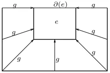
Figure 1: The action of an element g∈π1(Y) on ane∈π2(X, Y).

invariant (subsections 4.1. and 4.2). In section 4.3 we introduce the notion of an Eis-ermann lifting, namely a Reidemeister pair derived from a central extension of groups which reproduces the arc colourings of the Eisermann quandle, combined with addi-tional information on the crossings. We give a simple example of an Eisermann lifting that is strictly stronger than the Eisermann invariant it comes from. Finally, in sub-section 4.4, we give a homotopy interpretation of the Eisermann liftings, by using the notion of non-abelian tensor product and non-abelian wedge product of groups, defined by Brown and Loday [6, 7].

2.

Crossed modules of groups and categorical groups

2.1. Definition of crossed modules and first examples

Definition 2.1(Crossed module of groups).A crossed module of groups, G= (∂:E→G, ⊲), is given by a group morphism∂:E→Gtogether with a left action ⊲of GonE by

automorphisms, such that the following conditions (called Peiffer equations) hold: 1. ∂(g ⊲ e) =g∂(e)g−1_{; ∀g∈G,∀e∈E, 2. ∂(e)⊲ f =ef e}−1_{; ∀e, f ∈E.}

The crossed module of groups is said to be finite, if both groupsGandE are finite. Morphisms of crossed modules are defined in the obvious way.

Example 2.2. Any pair of finite groupsGandE, withEabelian, gives a finite crossed module of groups with trivial∂, ⊲(i.e.∂(E) = 1, g ⊲ e=e,∀g∈G,∀e∈E). More gen-erally we can choose any action ofGonEby automorphisms, with trivial boundary map∂:E→G.

Example 2.3. LetGbe any finite group. Let Ad denote the adjoint action ofGonG. Then (id :G→G,Ad) is a finite crossed module of groups.

Example 2.4. There is a well-known construction of a crossed module of groups in algebraic topology, namely the fundamental crossed module associated to a pointed pair (X, Y) of path-connected topological spaces (X, Y), thus Y ⊂X, namely the crossed module: Π2(X, Y) = (∂:π2(X, Y)→π1(Y), ⊲), with the obvious boundary

map∂:π2(X, Y)→π1(Y), and the usual action of π1(Y) onπ2(X, Y); see figure 1,

and [4] for a complete definition. This is an old result of Whitehead [30, 31].

Example 2.5. We may construct a topological pair (XD, YD) from a link diagramD of a linkK in S3_{, and thus obtain a crossed module Π}

2(XD, YD), associated to the diagram. Regard the diagram as the orthogonal projection onto thez= 0 plane in

S3_=R3_{∪ {∞}of a linkK}

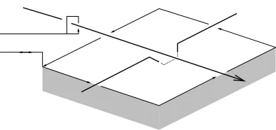
Figure 2: A generator ofπ1(YD) and a generator ofπ2(XD, YD).

the vicinity of each crossing point, where the undercrossing part of the link descends to height z=−1. Then we take XD (an excised link complement) to be the link complementCK ofKDminus an open ball, andYDto be thez>0 subset ofXD, i.e.

XD:= S3\n(KD))∩{(x, y, z)|z>−2}, YD:=XD∩ {(x, y, z)|z>0}, where n(KD) is an open regular neighbourhood of KD in S3. Note that the space

XDdepends only onK itself, so we can write it asXK. The same is not true forYD. Each arc of the diagram D corresponds to a generator of π1(YD) and there are no relations between generators. Each crossing of the diagram D corresponds to a generator of π2(XD, YD), namely ǫ: [0,1]2→XD, where the image under ǫ of the interior of [0,1]2 _{lies entirely in the region z <0 and the image of the boundary of}

[0,1]2_{, a loop contained inY}

D, encircles the crossing as in Figure 2. This boundary loop is the product of four arc loops inπ1(YD). Again there are no (crossed module) relations between the generators ofπ2(XD, YD) associated to the crossings. (This can be justified by Whitehead’s theorem [30, 31, 4]: for path-connected spaces X, Y, if

X is obtained fromY by attaching 2-cells, then Π2(X, Y) is the free crossed module

on the attaching maps of the 2-cells. Note that XD is homotopy equivalent to the CW-complex obtained fromYD by attaching a 2-cell for each crossing).

We observe that the quotientπ1(YD)/im∂is isomorphic to the fundamental group of the link complement CK=π1(S3\n(K)) for any diagram D, since quotienting

π1(YD) by im∂ corresponds to imposing the Wirtinger relations [8], which produces the Wirtinger presentation ofπ1(CK), coming from the particular choice of diagram. Thus Π2(XD, YD), whilst not being itself a link invariant (unless [15, 16] consid-ered up to crossed module homotopy), contains an important link invariant, namely

π1(CK), by taking the above quotient. The guiding principle in the construction to follow is to extract additional Reidemeister invariant information from the crossed module Π2(XD, YD).

2.2. A monoidal categoryC(G) defined from a categorical group G

It is well-known that a crossed module of groupsGgives rise to a categorical group, denotedC(G), a monoidal groupoid where all objects and arrows are invertible, with respect to the tensor product operation; see [2, 4, 1, 14, 21]. We recall the essential details. Given a crossed module of groupsG= (∂: E→G, ⊲), the monoidal category

these morphisms as downward pointing arrows and / or to represent them as squares - see (1).

U

(U,e)

V

or

U

e

V

, with∂(e)U =V.

(1)

The composition of morphismsU →e V andV →f W is defined to beU −→f e W, and the monoidal structure⊗is expressed asU ⊗V =U V on objects, and, on morphisms,

as: _

  

U

(U,e)

  y V

   ⊗

   

W

(W,f)

  y X

   =

U W  

y U W,(V ⊲f)e

W X

.

These algebraic operations are shown using squares in (2) and (3). U

e V

f W

=

U

f e

W

(2)

U

e V

⊗

U′

e′ V′

=

U U′

(V ⊲e′_)e V V′

(3)

The (strict) associativity of the composition and of the tensor product are trivial to check. The functoriality of the tensor product (also known as the interchange law) follows from the 2nd Peiffer equation. This calculation is done for example in [2, 4, 26].

Letκbe any commutative ring. The monoidal categoryC(G) has aκ-linear version

Cκ(G), whose objects are the same as the objects of C(G), but such that the set of morphisms U →V in Cκ(G) is given by the set of all κ linear combinations of morphisms U →V in C(G). The composition and tensor product of morphisms in

Cκ(G) are the obvious linear extensions of the ones in C(G). It is easy to see that

Cκ(G) is a monoidal category. The categorical group formalism is very well matched to the category of tangles to be used in the next section.

3.

Reidemeister

G

colourings of oriented tangle diagrams

3.1. Categories of tangles

Tangles are a simultaneous generalization of braids and links. We follow [24, 20] very closely, to which we refer for more details. Recall that an embedding of a manifold

Figure 3: A tangle with source + +−−with with target +−.

Figure 4: Elementary generators of tangle diagrams.

Definition 3.1. An oriented tangle [20, 28, 24] is a 1-dimensional smooth oriented manifold neatly embedded in R_×R_{×[−1,1], such that ∂(T)⊂}N_{× {0} × {±1}. A}

framed oriented tangle is a tangle together with a choice of a framing in each of its components [20, 24]. Alternatively we can see a framed tangle as an embedding of a ribbon intoR_×R_{×[−1,1], [27, 28, 11].}

Definition 3.2. Two oriented tangles (framed oriented tangles) are said to be equiv-alent if they are related by an isotopy ofR_×R_{×[0,1], relative to the boundary.}

Definition 3.3. A tangle diagram is a diagram of a tangle in R_{×[−1,1], obtained}

from a tangle by projecting it ontoR_{× {0} ×[−1,1]. Any tangle diagram}

unambigu-ously gives rise to a tangle, up to equivalence.

We have monoidal categories of oriented tangles and of framed oriented tangles [20, 28], where composition is the obvious vertical juxtaposition of tangles and the tensor product T⊗T′ _{is obtained by placingT}′ _{on the right hand side of T. The}

objects of the categories of oriented tangles and of framed oriented tangles are words in the symbols{+,−}; see figure 3 for conventions.

An oriented tangle diagram is a union of the tangle diagrams of figure 4, with some vertical lines connecting them. This is a redundant set if we consider oriented tangles up to isotopy.

Definition 3.4. A sliced oriented tangle diagram is an oriented tangle diagram, sub-divided into thin horizontal strips, inside which we have only vertical lines and pos-sibly one of the morphisms in figure 5.

X+ X− ∪

←

∪ ∩ ←∩

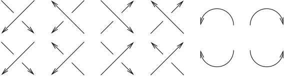
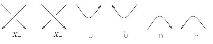
Figure 5: Generators for the categories of oriented tangles and of framed oriented tangles.

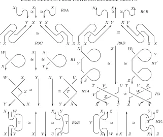
Theorem 3.5. The monoidal category of oriented tangles is equivalent to the monoidal category presented by the six oriented tangle diagram generators :

X+, X−, ∪,

←

∪,∩,←∩, (4)

shown in Figure 5, subject to the 15 tangle diagram relationsR0A−D,R1,R2A−C, R3 of Figure 6. The category of framed oriented tangles has the same set (4) as generators, subject to the 15 relationsR0A−D,R1′_{,R2A−C,R3of Figure 6.} Remark 3.6. We have replaced the R3 relation of Kassel’s theorem with its inverse, since this is slightly more convenient algebraically. The two forms of R3 are equivalent because of the R2A relations. The six other types of oriented crossing in figure 4, with one or both arcs pointing upwards, can be expressed in terms of the generators (4) and are therefore not independent generators - see [20], Lemma XII.3.1.

The previous theorem gives generators and relations at the level of tensor cate-gories. If we want to express not-necessarily-functorial invariants of tangles it is more useful to work with sliced tangle diagrams. The following appears for example in [24]:

Theorem 3.7. Two sliced oriented tangle diagrams represent the same oriented tan-gle (framed oriented tantan-gle) if, and only if, they are related by

1. Level preserving isotopies of tangle diagrams.

2. The moves R0A−R0D,R1,R2A−R2C, R3 of Figure 6 (in the case of tan-gles), performed locally in a diagram, or the moves R0A−R0D,R1′_,R2A− R2C,R3of Figure 6, in the case of framed tangles.

3. The “identity” and “interchange” moves of figure 7. (Here T andS can be any tangle diagrams and a trivial tangle diagram is a diagram made only of vertical lines.)

Definition 3.8 (Enhanced tangle). Let X be a set (normally X will be either a group or a quandle / rack). AnX-enhanced (framed) oriented tangle is a (framed) oriented tangle T together with an assignment of an element ofX to each point of the boundary of T. We will consider X-enhanced (framed) tangles up to isotopy of

R_×R_{×[−1,1], fixing the end-points.}

Given a setX, there exist monoidal categories having as morphisms the set ofX -enhanced oriented tangles and ofX-enhanced framed oriented tangles, up to isotopy. These categories have as objects the set of all formal wordsω in the symbolsaand

∼

= ∼= ∼= ∼=

∼

= ∼=

∼

= ∼=

∼

=

∼

=

∼

=

∼

= _∼

=

∼

= ∼= ∼= ∼=

R0A _R0B

R0C R0D

R1

R1′

R2A

R3

R2B R2C

Figure 6: Relations for the categories of oriented tangles and of framed oriented tangles.

trivial tangle diagram

trivial tangle diagram

trivial tangle diagram

trivial tangle diagram

trivial tangle diagram

trivial tangle diagram T

T

T

S T

S

∼

=

∼

=

a b c d

e f

Figure 8: AnX-enhanced tangle with source a.b.c∗_.d∗ _{and targete.f}∗_.

Definition 3.9. LetGbe a group. There exists an evaluation mapω7→e(ω), which associates to a wordωinG⊔G∗_{an element ofG, obtained by multiplying all elements}

ofωin the same order, by puttingg∗₌. _g−1_{(ande(∅) = 1}

G for the empty word∅).

3.2. Colourings of tangle diagrams

LetG= (∂:E→G, ⊲) be a crossed module of groups. We wish to define the notion of aG-colouring of an oriented tangle diagram, by assigning elements ofGto the arcs and elements ofE to the crossings in a suitable way.

For a link diagramDrealized as a tangle diagram, aG-colouring may be regarded as a morphism of crossed modules from the fundamental crossed module Π2(XD, YD) of Example 2.5, toG. This idea extends in a natural way to general tangle diagrams.

Definition 3.10. Given a finite crossed moduleG= (∂:E→G, ⊲) and an oriented tangle diagramD, aG-colouring ofDis an assignment of an element ofGto each arc of the diagram, and of an element ofE to each crossing of the diagram, such that, at each crossing of typeX+ or X− with colourings as in (7), the following relations

hold:

X+: ∂(e) =XY X−1Z−1 (5)

X−: ∂(e) =Y XZ−1X−1 (6)

Z ## G G G G G G G G G X {{ wwww wwww wwww wwww wwww e ## G G G G G G G G G X Y X ## G G G G G G G G G G G G G G G G G G G G Z {{ wwww wwww w e {{ wwww wwww w Y X (7)

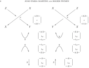
Thus we are assigning to each type of coloured crossing a morphism ofC(G) and ofCκ(G), and in a similar way we may associate morphisms ofC(G) to all elementary

G-coloured tangles, as summarised in figure 9. With the duality where the dual of the morphismX−→e ∂(e)X isX−1_∂(e)−1_{−−−−→}X−1⊲e _X−1_{, and the morphisms associated to}

Z ## G G G G G G G G G X {{ wwww wwww wwww wwww wwww e ## G G G G G G G G G X Y ZX e XY X ## G G G G G G G G G G G G G G G G G G G G Z {{ wwww wwww w e {{ wwww wwww w Y X XZ e Y X X

JJ XX¯

1E

1G

X

TT XX¯

1E 1G X 1G 1E ¯ XX X 1G 1E XX¯

X X 1E X X

OO _X¯

1E

¯

X

Figure 9: TurningG-coloured tangles into morphisms of C(G) The symbol ¯X stands forX−1_.

Thus we can assign to the completeG-coloured oriented tangle diagram a morphism ofC(G), by using the monoidal product horizontally and composition vertically. This leads to the following definition:

Definition 3.11. Given aG-colouringF of a tangle diagramD (we sayF ∈CG(D), the set ofGcolourings ofD), the evaluation ofF, denotede(F), is the morphism in

C(G) obtained by multiplying horizontally and composing vertically the morphisms ofC(G) associated to the elementary tangles which make upD.

Remark 3.12. For a link diagram the evaluation ofF takes values inA, the automor-phism subgroup of 1G, i.e.A= ker∂⊂E.

For a tangle diagram without open ends at the top and bottom, i.e. a link diagram, one can conjecture that the number ofG-colourings of the diagram can be normalized to a link invariant, by analogy with the familiar link invariant which is the number of Wirtinger colourings of the diagram using a finite groupG(a Wirtinger colouring in the present context would be aG-colouring where the groupE is trivial). Indeed it was proven in [14] that the number of colourings of a link diagram evaluating to the identity ofE can be normalised to give an invariant of knots. However this invariant depends only on the homotopy type of the complement of the knot [15], thus it is a function of the knot group only.

G-colourings does respect the Reidemeister moves. Intuitively we are looking at the simple homotopy type, rather than the homotopy type of a link complement. Our idea is to restrict ourselves toG-colourings of diagrams where, at each crossing, the colouring of the crossing with an element ofE is determined by theG-colouring of two arcs, namely the overcrossing arc and the lower undercrossing arc. To this end we introduce two functions:

ψ:G×G→E, φ:G×G→E,

which determine theE-colouring of the two types of crossing, as in (8):

Z

@ @ @ @ @ @ @

ψ(X,Y)

X

~~

~~~~ ~~~~

~~~~ ~~~~

@ @ @ @ @ @ @

X Y

X

@ @ @ @ @ @ @ @ @ @ @ @ @ @ @ @

φ(X,Y)

Z

~~

~~~~ ~~~

~~

~~~~ ~~~

Y X

(8)

Since this is aG-colouring, these functions determine theG-assignment for the remain-ing arc:

X+: Z=∂ψ(X, Y)−1XY X−1 (9)

X−: Z=X−1∂φ(X, Y)−1Y X (10) We now come to our main definition.

Definition 3.13(unframed Reidemeister pair).The pair Φ = (ψ, φ) is said to be an unframed Reidemeister pair ifψ:G×G→Eandφ: G×G→Esatisfy the following three relations for eachX, Y, T ∈G:

ψ(X, X)R= 11 E (11)

φ(X, Y)ψ(X, Z)R= 12 E (12)

φ(Y, X).Y ⊲ φ(T, Z).φ(T, Y)R=3X ⊲ φ(T, Y).φ(T, X).T ⊲ φ(V, W) (13) where, in R2,Z=X−1_{∂φ(X, Y)}−1_{Y X, and in R3:}

Z=Y−1∂φ(Y, X)−1XY , V =T−1∂φ(T, Y)−1Y T , W =T−1∂φ(T, X)−1XT Remark 3.14. The equations above relate to the Reidemeister 1-3 moves, as we will see shortly in the proof of Theorem 3.19. If equation (12) holds we can substitute (13) by the equivalent:

ψ(X, Y). A ⊲ ψ(X, Z). ψ(A, B) =X ⊲ ψ(Y, Z). ψ(X, C). D ⊲ ψ(X, Y) (14) where:

A=∂(ψ(X, Y))−1XY X−1 , B=∂(ψ(X, Z))−1XZX−1 , C=∂(ψ(Y, Z))−1Y ZY−1 , D=∂(ψ(X, C))−1XCX−1 .

Z f(Z)

f(Z)

f(Z)

φ(f(Z),Z)

A A

A g(A)

ψ(A,A)

Figure 10: Definition off, g:G→G.

1. GivenZinG, the equation (c.f. left of figure 10)∂(φ(A, Z))A=Zhas a unique solutionf(Z)∈G.

2. Defining g(A) =∂(ψ(A, A))−1_{A (c.f. right of figure 10) it holds that f◦g=}

g◦f = id. In particular both f andgare bijective.

Definition 3.16. Given a crossed module G= (∂:E→G, ⊲), with G finite, pro-vided with a (framed or unframed) Reidemeister pair Φ = (ψ, φ), and an oriented

G-enhanced tangle diagramD, a ReidemeisterG-colouring ofDis aG-colouring ofD

(which extends the colourings at the end-points ofD, in the sense that an arc coloured byg corresponds to endpoints coloured by g or g∗_{, depending on the orientation}

-see Figure 8) determined by the functionsψ:G×G→E, φ:G×G→E, which fix the colourings at each crossing as in (8), (9) and (10).

We are now in a position to define a state-sum coming from the Reidemeister

G-colourings of a link diagramD. Recall Definitions 3.9 and 3.11.

Definition 3.17. Consider a crossed moduleG= (∂:E→G, ⊲), withGfinite, pro-vided with a (framed or unframed) Reidemeister pair Φ = (ψ, φ). Consider an oriented

G-enhanced tangle diagramD, connecting the wordsω andω′ _inG⊔G∗_{. We denote}

the corresponding set of ReidemeisterG-colourings of D by CΦ(D, ω, ω′). Then we

define the state sum:

IΦ(D) =hω|IΦ(D)|ω′i=.

X

F∈CΦ(D,ω,ω′)

e(F) (15)

taking values in N_{HomC(G) e(ω), e(ω}′_)⊂Hom

C_Z(G) e(ω), e(ω′). (Here the set of

morphismsx→y in a categoryC is denoted by HomC(x, y).)

Remark 3.18. If D is a link diagram then IΦ(D) takes values in Z[A], the group

algebra ofA= ker∂.

Theorem 3.19.The state sum IΦ defines an invariant of G-enhanced tangles if Φ

is an unframed Reidemeister pair and an invariant of framedG-enhanced tangles if

Φis a framed Reidemeister pair.

Proof. To prove this result, we need to show thatIΦrespects the relations of Theorem

∼

= ∼= ∼= ∼=

∼

= ∼=

∼

= ∼=

∼

=

∼

=

∼

=

∼

= _∼

=

∼

= ∼= ∼= ∼=

R0A _R0B

R0C R0D

R1

R1′

R2A

R3

R2B R2C

X X X X X X

Y X

X Z

Y X

X Z Z X

X Y

Z X X Y

W

X

X X

Y

X

Y

Z

Z W

V

Z

W X

Y

Z

X

Y X Y U

T

Y X

T V U

Y _Z

X Y T

T V Z W

X Y T

X Y Z X W

X Y U Y T X Y

X W Y

X Z

X Z X Z

T U Z

Figure 11: Tangle relations withG-assignments to the arcs.

and then show that the corresponding morphisms ofC(G) are equal (and in some cases, that the remaining arcs connecting to the exterior are also coloured compatibly). Thus for a pair of diagrams related by one of the relations, each term in the expression for

IΦ for one diagram has a corresponding term in the expression for IΦfor the other

diagram, and the evaluations are equal term by term.

R0A and R0B: FixX∈G. The corresponding equation in E is 1E = 1E in each case.

R0C: FixX, Y ∈G. The corresponding equation inE: (X−1Z−1)⊲ ψ(X, Y) = (Y−1X−1)⊲ ψ(X, Y) is an identity which follows from:

ψ(X, Y) = (∂ψ(X, Y))⊲ ψ(X, Y) = (XY X−1Z−1)⊲ ψ(X, Y).

R0D: FixX, Y ∈G. The corresponding equation inE: (Z−1X−1)⊲ φ(X, Y) = (X−1Y−1)⊲ φ(X, Y) is an identity which follows from:

φ(X, Y) = (∂φ(X, Y))⊲ φ(X, Y) = (Y XZ−1X−1)⊲ φ(X, Y).

R2A: FixX, Y ∈G. The corresponding equation in E is:

where Z=X−1_{∂φ(X, Y)}−1_{Y X and T =∂ψ(Y, X)}−1_{Y XY}−1_{. The 1st equality is}

(12), and the 2nd equality follows from the 1st: ψ(X, Z)φ(X, Y) = 1E with Z =

X−1_{∂φ(Y, X)}−1_{XY, i.e.}

Y =∂φ(X, Y)XZX−1=∂ψ(X, Z)−1XZX−1,

then substitute variablesX7→Y, Z7→X, Y 7→T. Applying∂to (16), it follows that

W =Y andU =X.

R1: FixX ∈G. The corresponding equation in E is:

ψ(X, X) = 1E =φ(X, Y), ∂φ(X, Y) =Y X−1

The 1st equality is (11), implying W =X, and the 2nd equality follows from (11) and (16), see just below, which also impliesY =X.

φ(X, Y) =φ(X, Y)ψ(X, X)φ(X, X) =φ(X, X) = 1E.

R2B: FixX, Y ∈G. The corresponding equation inE for the left move is:

X−1⊲ φ(X, Y). X−1⊲ ψ(X, Z) = 1E

withZ =X−1_{∂φ(X, Y)}−1_{Y X, which is the 1st equality in (16). Applying∂, it follows}

thatW =Y. The equation inE for the move on the right:

U−1⊲ ψ(Y, T). X−1⊲ φ(Y, X) = 1E

with T =Y−1∂φ(Y, X)−1XY and U =∂ψ(Y, T)−1Y T Y−1, follows from the 2nd equality of (16) forX =∂ψ(Y, T)−1_{Y T Y}−1_{, and thereforeT =Y}−1_{∂ψ(Y, T)XY, or}

T =Y−1_{∂φ(Y, X)}−1_{XY, by acting withX}−1_=U−1_.

R2C: FixX, Z∈G. The corresponding equation in E:

Y−1⊲ φ(X, Y). Y−1⊲ ψ(X, Z) = 1E=Z−1⊲ ψ(Z, X). Z−1⊲ φ(Z, T) (17) with Y =∂ψ(X, Z)−1_XZX−1 _{and T =∂ψ(Z, X)}−1_ZXZ−1_{, is equivalent to (16)}

with Y substituted by Z in the 2nd equality. Applying ∂ to (17), it follows that

W =Z andU =X.

R3: FixX, Y, T ∈G. The corresponding equation inEis the Reidemeister 3 equa-tion (13), which also implies the equalityU =Z, by applying∂.

Invariance under the identity and interchange moves of Figure 7 is immediate - to show the latter we use the interchange law for the operations of Figures 2 and 3.

For framed tangles we need to show invariance ofIΦunder theR1′move using the

properties (i) and (ii) of Definition 3.15, which replace the Reidemeister 1 condition (11).

FixZ∈G. For the move on the left, at the lower crossing we have, from (i), the relationY =g(Z), and at the upper crossing we have the relationX =f(g(Z)) =Z, by (ii). The equation for the move, which isψ(Z, Z)φ(Z, Y) = 1E,follows from the 2nd equality in (16). For the move on the right, at the lower crossing we have, from (i), the relationV =f(Z), and at the upper crossing we have the relationW =g(f(Z)) =

Z, by (ii). The equation for the move, namelyφ(V, Z)ψ(V, V) = 1E follows from the 1st equality in (16).

We close this section by stating a TQFT property of the invariantIΦ, which follows

y ⊲ x y

y x

y x ⊳ y

x y

Figure 12: A rack colouring of a link diagram in the vicinity of a vertex.

Theorem 3.20.Let D1 andD2 be tangle diagrams, so that the vertical composition

D1

D2 is well defined. For any enhancementsωandω

′′_{of the top ofD}

1and the bottom

ofD2 we have:

ω

IΦ

D1

D2

ω′′

=X ω′

hω|IΦ(D1)|ω′i

hω′_|I

Φ(D2)|ω′′i ,

where the sum extends over all possible enhancements ω′ _{of the intersection of D}

1

withD2.

4.

Examples

4.1. Examples derived from racks and quandles

4.1.1. Rack and quandle invariants of links

Recall that a rack R is given by a set R together with two (by the axioms not independent) operations (x, y)∈R×R7→x ⊲ y∈Rand (x, y)∈R×R7→x ⊳ y∈R, such that for eachx, y, z∈R:

1. x ⊲(y ⊳ x) =y,

2. (x ⊲ y)⊳ x=y,

3. x ⊲(y ⊲ z) = (x ⊲ y)⊲(x ⊲ z),

4. (x ⊳ y)⊳ z= (x ⊳ z)⊳(y ⊳ z). A quandleQis a rack satisfying the extra condition:x ⊳ x=x=x ⊲ x,∀x∈Q. There is a more economical definition of a rack: it is a set R with an operation (x, y)7→x ⊳ y, such that condition (4) above holds and such that for eachy∈R the mapx7→x ⊳ y is bijective. Its inverse will give us the mapx7→y ⊲ x. The following result and proof appeared in [23].

Lemma 4.1 (Nelson Lemma). Given a rack R, the maps x7→x ⊲ x andx7→x ⊳ x are injective (thus bijective if the rack is finite.)

Proof. Letxandy belong toR. Then

(x ⊲ x)⊲ y= (x ⊲ x)⊲(x ⊲(y ⊳ x)) =x ⊲(x ⊲(y ⊳ x)) =x ⊲ y.

Ifx ⊲ x=y ⊲ y thenx ⊲ x= (x ⊲ x)⊲ x= (y ⊲ y)⊲ x=y ⊲ x.Sincey ⊲ y=x ⊲ xthen

y ⊲ y=y ⊲ x. This impliesx=y, since the mapx7→y ⊲ xis bijective, its inverse being

x7→x ⊳ y. The proof forx7→x ⊳ x is analogous.

Given a knot diagramD, and a rackR, a rack colouring ofD is an assignment of an element ofR to each arc of D, which at each crossing of the projection has the form shown in figure 12.

Theorem 4.2. Let R be a finite rack. Then the number IR(D) of rack colourings

of a link diagram D is invariant under the Reidemeister moves 1’, 2 and 3, and is therefore an invariant of framed links, also calledIR. Moreover ifRis a quandle then

the number of rack colourings is invariant under the Reidemeister 1 move, therefore defining a link invariant.

For a proof see [23] or [17]. (Invariance under the Reidemeister moves 2 and 3 is immediate. Invariance under the Reidemeister 1’ move, which is less trivial, is a consequence of the Nelson Lemma.)

4.1.2. Reidemeister pairs derived from racks and quandles

Let us see that rack and quandle invariants can be written in the framework of this article. LetRbe a rack, which we suppose to be finite. Consider an arbitrary group structure onR. Call the groupG. We do not impose any compatibility relation with the rack operations, we just assume that the underlying set ofR coincides with the underlying set of G. Consider the crossed module G= (id :G→G,ad), where ad denotes the adjoint action ofGonG. Put:

ψ(b, a) =b a b−1(b ⊲ a)−1 , φ(b, a) =a b(a ⊳ b)−1b−1. (18)

Theorem 4.3. The pairΦ = (ψ, φ)is a framed Reidemeister pair. MoreoverΦis an unframed Reidemeister pair ifR is a quandle.

Proof. In this case relation R2 reads, φ(b, a)ψ(b, a ⊳ b) = 1 which follows

tautologi-cally. The relationR3reads in this case:

φ(b, a). bφ(c, a ⊳ b)b−1. φ(c, b) =aφ(c, b)a−1. φ(c, a). cφ(b ⊳ c, a ⊳ c)c−1,

and follows easily, from relation (3) of the definition of a rack.

Let us now prove relations (i) and (ii) of Definition 3.15. Leta∈G. The equation

z=∂(φ(a, z))ameansz=z a(z ⊳ a)−1_{,orz ⊳ a=a, that isz=a ⊲ a. By the Nelson}

Lemma 4.1, for eachzthe equationz=a ⊲ ahas a unique solutionf(z)∈R. In this caseg(a) =∂(ψ(a, a))−1_{a=a ⊲ a. Thus triviallyf ◦g=g◦f = id}

R. Finally ifR is a quandle thenψ(x, x) =x(x ⊲ x)−1_{=x x}−1_{= 1}

E.

Since there is clearly, by (8), (9) and (10), a one-to-one correspondence between

G-colourings of a link diagram D and rack colourings (with respect to R) of D, we have:

Theorem 4.4. Given a link diagramD, we haveIΦ(D) =IR(D)1G,where1G is the

identity of G. Therefore the class of invariants defined in this paper is at least as strong as the class of rack link invariants.

There is a spin-off of the rack invariant in order to handle tangles. Given a rack

R, recall that anR-enhanced tangle, Definition 3.8, is a tangle together with a map from the boundary of T into (the underlying set of) R. There is a category whose objects are the words ω in R⊔R∗ _{and whose morphisms are R-enhanced tangles}

connecting them. Thus if the wordω is the source of T then ω is a word having i

elements, whereiis the number of intersections of the tangle withR2_{× {1}. Moreover}

thenth _{element of ω is either the colour a∈R given to then-th intersection, or it}

associated strand is pointing upwards. These conventions were explained in figure 8. Given anR-enhanced tangleT letω(T) andω′_{(T) be the source and target ofT, both}

words inR⊔R∗_{. Definehω(T)|I}

R(T)|ω′(T)ias being the number of arc-colourings of a diagram ofT extending the enhancement ofT. This defines an invariant of tangles, for any choice of colourings on the top and bottom of T (in other words, for any

R-enhancement ofT). Clearly

Theorem 4.5. For anyR-enhanced tangle T, puttingω=ω(T) andω′ _=ω′_{(T) we} have (see definitions 3.9 and 3.11 for notation):

hω(T)|IΦ(T)|ω′(T)i=hω|IR(T)|ω′i

e(ω)

 

ye(ω′_)e(ω)−1

e(ω′₎ .

4.1.3. Reidemeister pairs derived from rack and quandle cocycles

We can extend the statement of Theorem 4.4 for the case of rack cohomology invari-ants of knots. Let R be a rack. Let V be an abelian group. We say that a map

w:R×R→V is a rack 2-cocyle if:

w(x, y) +w(x ⊳ y, z) =w(x, z) +w(x ⊳ z, y ⊳ z), for eachx, y, z∈R.

IfR is a quandle, such awis said to be a quandle cocycle if moroeverw(x, x) = 0V, for eachx∈R. For details see [10, 9, 23, 12, 13].

Consider any group structure G on the set R, which may be completely inde-pendent of the rack operations. Consider the crossed module (∂: G×V →G,•), whereg•(h, v) = (ghg−1, v), for eachg, h∈Gandv∈V,which is a left action ofG

onG×V by automorphisms, and∂(g, v) =g, for each (g, v)∈G×V. Given a rack 2-cocyclew:R×R→V, set:

ψ(b, a) = b a b−1(b ⊲ a)−1, w(b ⊲ a, b), φ(b, a) = a b(a ⊳ b)−1 b−1, w(a, b)−1.

Theorem 4.6. The pair Φ = (ψ, φ) is a framed Reidemeister pair. Its associated framed link invariant coincides with the usual rack cohomology invariant of framed links. Morever if R is a quandle and w a quandle 2-cocycle then Φ = (ψ, φ) is an unframed Reidemeister pair and its associated invariant of links coincides with the usual quandle cocycle link invariants [10_].

Proof. Analogous to the proof of Theorems 4.3 and 4.4.

Therefore the class of invariants defined in this paper is at least as strong as the class of invariants of links derived from quandle cohomology classes.

4.2. Relation with the Eisermann knot invariant

4.2.1. String knots, long knots, knot meridians and knot longitudes

Recall that an (oriented) long knot is an embedding f ofR _into R3_{. such that, for}

K LK K′ LK′

Figure 13: Turning an oriented knot into a string knot in two different cases.

There exists an obvious closing map, cl, sending a string knotLto a closed knot cl(L). It is well known that this defines a one-to-one correspondence between isotopy classes of string knots and isotopy classes of oriented knots. To see this, note that a map sending a closed knot K to a long knot LK can be obtained by choosing a base point p∈K. Then there exists an (essentially unique) orientation (of S3 _and

ofK) preserving diffeomorphism (S3\ {p}, K\ {p})→(R3, Lp_K), whereLp_K is a long knot with cl(Lp_K) =K. Note that Lp_K depends only on the orientation preserving diffeomorphism class of the triple (S3_{, K, p), thus since all pairs (K, p), with fixedK,}

but arbitrary p, are isotopic we can see that Lp_K depends only on K, thus we can write it asLK.

LetD be a knot diagram of the knotK. Consider the Wirtinger generators of the fundamental groupπ1(CK) of the complementCK=S3\n(K) of K (heren(K) is an open regular neighbourhood of K); we thus have a meridian for any arc of the diagram D. Let a be an arc of D and p a base point of K in a. Then there is a meridian mp=m of K encircling the arc aat p, whose direction is determined by the right hand rule. LetD2_{={z∈C:|z|61}andS}1_=∂D2_{. Choose an embedding}

f:S1_×D2_→S3 _{such that}

• f(S1_{× {0}) =K, preserving orientations, withf(1,0) =p.}

• f({1} ×S1_{) =m}

• f(S1_{× {1}) has zero linking number withK.}

If we take f(1,1) to be the base point of S3_{, then the homotopy class l}

p=l∈

π1(CK) off(S1× {1}) is called a longitude ofK[8]. It is well known that the triple (π1(CK), m, l), considered up to isomorphism, is a complete invariant of the knotK [29]. Note that if we choose another base point p′ _{of K then m}

p′ and l_p′ can be

obtained frommp andlp by conjugating by a single element ofπ1(CK).

The longitudelp, being an element of the fundamental group of the complement

CK ofK, can certainly be expressed in terms of the Wirtinger generators. This can be done in the following way; for details see [12, 13]. Let a0=abe the arc of the

diagram D of K containing the base point of K. Then go around the knot in the direction of its orientation. This makes it possible to order the arcs of K, say as

a1, a2, . . . , an; we would havean=a1, except that we prefer to seeK as being split

at the base pointp, separating the arca in two. We can also order the crossings of

D.

aj

ai

ai+1

aj ai

ai+1

li=ga1li+1l

−1

j gal−1lj =ga1li+1g

−1

aj

li+1=lig−ai1gaj

li=ga−11li+1l

−1

j gallj =g−a11li+1gaj

li+1=ligaig−aj1

or or

Figure 14: Rules for partial longitudes at crossings.

element of the fundamental group of the complement byga. Then clearly we have that

gai =l−i 1ga1li. The way to pass fromli to li+1 appears in figure 14 for the positive and negative crossing.

Giveni, letjibe the number of the arc splittingai andai+1. Letθibe the sign of thei-th crossing. Then:

l= n_Y−1

i=1

g−θi ai gθiaji =

n_Y−1

i=1

l−_i 1g−θi a1 lil

−1

ji gaθi1lji= n_Y−1

i=1

[l_i−1, g−θi a1 ] [g

−θi a1 , l

−1

ji ]; (19) more generally, ifk∈ {2, . . . , n}:

lk = k_Y−1

i=1

gai−θigaθi_ji = k_Y−1

i=1

l−i 1g−a1θilil

−1

ji gθia1lji = k_Y−1

i=1

[li−1, ga−1θi] [g

−θi a1 , l

−1

ji ]. (20) Thus both the longitudeland any partial longitudelkbelong to the commutator sub-group of the fundamental sub-group of the complement ofK. Alsoli+1=li[l−i1, g−a1θi] [g

−θi a1 , l

−1

ji ]. In remark 4.13 we will present another formula for a knot longitude.

4.2.2. The Eisermann invariant of knots

LetK be a knot in S3_{. Consider the fundamental group of the complement C}

K =

S3_{\n(K) of the knotK. Heren(K) is an open regular neighbourhood ofK. Choose}

a base pointpof K. Let the associated meridian and longitude of K in π1(CK) be denoted bymp andlp, respectively. Note that [mp, lp] = 1.

Let f: π1(CK)→G be a group morphism. Therefore f(lp)∈G′= [. G, G], the derived (commutator) group ofG, generated by the commutators [g, h]=. ghg−1_h−1_.

Moreover [f(lp), f(mp)] = 1G. Then

f(lp)∈Λ= [. G, G]∩C(x),

wherex=f(mp) andC(x) is the set of elements ofGcommuting withx.

LetGbe a finite group. Letxbe an element ofG. The Eisermann invariant [13] (also called Eisermann polynomial) is:

E(K) = X

{f:π1(CK)→G|f(mp)=x}

f(lp)∈N(Λ).

mp′ =h m_ph−1 and l_p′ =h l_ph−1, for some common h∈π₁(C_K). The Eisermann

invariant can be used to detect chiral and non invertible knots [13]. ClearlyE(K) is given by a mapfK

E:G′ →N, where

E(K) = X g∈G′

fEK(g)g.

Note thatfK

E(g) = 0 ifg6∈Λ.

Let us see that the Eisermann invariant can be addressed using Reidemeister pairs. This is a consequence of the previous subsections and the discussion in [13, 12], which we closely follow, having discussed and completed the most relevant issues in 4.2.1.

LetG be a group. Choose x∈G and consider from now on the pair (G, x). We will use the notationhg_=g−1_{hg, whereg, h∈G. Let}

Q=xg, g∈G′ ⊂G, Q=xg, g∈G ⊂G.

Lemma 4.7. Both setsQand Qare self conjugation invariant:

a, b∈Q =⇒ a−1ba∈Q and a, b∈Q =⇒ a−1ba∈Q ThereforeQandQ are both quandles, with quandle operationh ⊳ g=hg_.

Proof. Giveng, h∈G′_{we have (g}−1_xg)−1_(h−1_xh)(g−1_{xg) =x}x−1_hg−1_xg

,andx−1_hg−1_xg=

x−1_hg−1_xgh−1_{h= [x}−1_{, hg}−1_]h∈G′_{. The proof forQis analogous.}

It is easy to see that:

Lemma 4.8 (Eisermann). Let Gbe a group. Given arbitraryx∈G, bothG′ _{and G} are quandles, with quandle operation:

h ⊳ g=x−1hg−1xg , g ⊲ h′=xh′g−1x−1g. (21)

There are also quandle mapsp:G′_{→Qand p:Q→Gwithp(g) =x}g_. Recall the rack invariant of tangles, defined just before Theorem 4.5.

Theorem 4.9 (Eisermann).For any knot K and any g inG′ _{it holds that:} h1G|IG′(DK)|gi=fEK(g),

where DK is any string knot diagram associated to K. Of course we regard DK as

a G-enhanced tangle diagram coloured with 1G= 1G′ at the top and with g at the bottom.

Proof. Follows from the discussion in 4.2.1 and especially figure 14.

Remark 4.10. The previous theorem is also valid for the quandle structure in G, Lemma 4.8. Given the form of the quandle is easy to see that ifg, h∈G′_:

hg|IG′(D_K)|hi=hg|I_G(D_K)|hi.

By using subsection 4.1 we will show that the Eisermann invariant can be addressed in our framework, by passing to string knots. Suppose we are given a finite groupG

in the underlying set ofG′_{. We take the most obvious one, given by the inclusionG}′ _⊂ G. The associated crossed module isG′ _→id _G′_{, withG}′_{acting on itself by conjugation.}

Define, giveng, h∈G′_{, the pair Φ}x_{= (ψ}x_{, φ}x_{), as:}

φx(g, h) =hg(xg)−1xhh−1g−1=hx−1gh−1xg−1= [hx−1, gx−1]

ψx_{(g, h) = [g, h][hg}−1_{, x] = [xhg}−1_x−1_gx−1_{, gx}−1_]−1 (22) Theorem 4.11.The pair Φx_{= (ψ}x_{, φ}x_{) is an unframed Reidemeister pair for the}

crossed moduleG′_→id _G′_{, withG}′ _{acting on itself by conjugation. LetKbe an oriented} knot andLK be the associated string knot. Giveng∈G′ then

h1G′|IΦx(L_K)|gi=fK

E(g). (23)

Proof. The expressions for Φx_{= (ψ}x_{, φ}x_{) guarantee that the colourings of the arcs} at a crossing are those given by the Eisermann quandle operation and its inverse (Lemma 4.8). Thus equation (23) holds, and it is enough to check that Φ does indeed satisfy the conditions to be a unframed Reidemeister pair. Clearly the Rei-demeister 1 condition (11) holds:ψx_{(l, l) = 1. The Reidemeister 2 equation (12) is:}

φx_{(l, m)ψ}x_{(l, x}−1_ml−1_{xl) = 1, i.e.}

[mx−1, lx−1] [l, x−1ml−1xl] [x−1ml−1x, x] = 1.

Writing this out in full, one obtains:

mx−1lx−1xm−1xl−1. l(x−1ml−1xl)l−1(l−1x−1lm−1x).(x−1ml−1x)x(x−1lm−1x)x−1

=m x−1lm−1xl−1. lx−1ml−1x l−1x−1lm−1x . x−1ml−1xl m−1= 1.

In the above computation, the underlined factors are equal to 1.

To avoid confusion with the quandle operation ⊲, the left action of G′ _{on G}′

by conjugation will be denoted by g•h, thusg•h=ghg−1 _{for each g, h∈G}′_{. The}

Reidemeister 3 equation (13) for this case reads:

φx(l, m). l•φx(n, p). φx(n, l) =m•φx(n, l). φx(n, m). n•φx(r, q),

where p=x−1_ml−1_{xl, r=x}−1_ln−1_{xn, q=x}−1_mn−1_{xn. The left-hand side of}

the above equation, written out in full, is:

mx−1lm−1xl−1. l(px−1np−1xn−1)l−1.(lx−1nl−1xn−1)

=m x−1lm−1x . x−1ml−1x lx−1n(l−1x−1lm−1x)xn−1. x−1nl−1xn−1

=mln(n−1_x−1_nl−1_x−1_lm−1_x2_)(n−1_x−1_nl−1_x)n−1_,

and the right-hand side leads to the same expression:

m(lx−1_nl−1_xn−1_)m−1_{. mx}−1_nm−1_xn−1_{. n(qx}−1_rq−1_xr−1_)n−1

=mlx−1nl−1xn−1x−1nm−1x(x−1mn−1xn). x−1 (x−1l n−1xn)(n−1x−1n m−1x)x(n−1x−1nl−1x)n−1

=mln(n−1_x−1_nl−1_x−1_lm−1_x2_)(n−1_x−1_nl−1_x)n−1_.

m l n

n r U

p

m l n

n r u

q

Figure 15: Two sides of the Reidemeister-III move in the proof of Theorem 4.11.

of the 6 external arcs in Figure 15 for Reidemeister 3, taken in anticlockwise order starting withm, where u is the colouring assigned to the rightmost upper arc, i.e.

u=x−1_pn−1_xn=x−1_qr−1_xr.

Consider the quandle structure inG, Lemma 4.8, given by the same formulae as the one of G′_{. Consider the crossed module given by the identity map G→Gand}

the adjoint action ofG onG. Givenx∈Gwe have an unframed Reidemeister pair ¯

Φx_{= ( ¯ψ}x_,φ¯x_{), with the same formulae as (22), namely:} ¯

φx_{(g, h) =hg(x}g₎−1_xh_h−1_g−1_=hx−1_gh−1_xg−1_{= [hx}−1_{, gx}−1_{] ,}

¯

ψx_{(g, h) = [g, h][hg}−1_{, x] = [xhg}−1_x−1_gx−1_{, gx}−1_]−1 (24)

forg, h∈G. It is easy to see that:

Proposition 4.12.Let a, b∈G′_{. For each x∈G, and each string knot L}

K:

ha|IΦx(L_K)|bi=ha|I_Φ¯x(L_K)|bi

Remark 4.13 (Formula for a knot longitude). Our approach for defining Eisermann invariants, and the proof of Theorem 4.11, provides a different formula to (19) for the longitudelp=l of a knotK, ifK is presented as the closure of a string knotL. It is assumed that the base pointp∈K of the closed knotKlives in the top end ofL. LetG=π1(CK). Consider the crossed module (id :G→G,ad). Letxbe the element ofGgiven by the top strandaof L. Let bbe the bottom strand ofL. Consider the Reidemeister pair ¯Φx _{in (24), thus}

¯

φx(g, h) = [hx−1, gx−1] and ψ¯x(g, h) = [g, h][hg−1, x] = [xhg−1x−1gx−1, gx−1]−1.

(25) Consider a diagramDofL. Colour each arccof the diagramDwith the corresponding partial longitudelc, as defined in 4.2.1. Thereforela= 1 andlb=l. Then by the proof of Theorem 4.11 one has a Reidemeister colouringF. If we evaluateF (definitions 3.9 and 3.11), we have a morphismla

e(F)

−−−→lb, hencee(F) =l=lp. The form ofe(F) thus yields an alternative formula for the knot longitude, which will be crucial for giving a homotopy interpretation of the lifting (Theorem 4.17) of the Eisermann invariant. 4.2.3. One example of Eisermann invariants

Let G be a group with a base point x. The explicit calculation of the invariant

h

g

xhg−1_x−1_g

x2_gh−1_x−1_hg−1_x−1_g

x3_hg−1_x−1_gh−1_x−1_hg−1_x−1_g

h g

x−1_hg−1_xg

x−2_g −1_xhg−1_{xg h}

x−3_hg−1_xg −1_xhg−1_{xg h}

Figure 16: The Eisermann polynomial for the positive and negative trefoil knotsK+

andK−

x id (12) (12)(34) (123) (123)(45) (1234) (12345)

K− id 7id 5id 7id id id + 4(13)(24) id + 5(12345)

K+ id 7id 5id 7id id id + 4(13)(24) id + 5(15432)

Table 1: The Eisermann invariant for the negative and positive trefoils forG=S5.

(the positive and negative trefoils), converted to string knots, appears in figure 16. In particular, givena, g, h∈G, we have:

ha|I_Φ¯x(K₊)|gi= #

h∈G:x3hg−1x−1gh−1x−1hg−1x−1g=a; x2gh−1x−1hg−1x−1g=h , ha|I_Φ¯x(K−)|hi= #

g∈G: x−3hg−1xgh−1xhg−1xg=g; x−2gh−1xhg−1xg=a .

Consider from now onG=S5. We refer to table 1, displaying the values ofh1|I_Φ¯x(K−)|ai and h1|I_Φ¯x(K+)|ai for some choices of x∈S5, representing all possible conjugacy

classes inS5. In each 2nd and 3rd row entry of table 1, we put:

X

h∈S5

h1|IΦ¯x(K−)|hi and

X

g∈S5

h1|IΦ¯x(K+)|gi,

both elements of the group algebra ofS5. Therefore the invariant L7→ h1|I_Φ¯x(L)|bi, where we identify a knot with its associated string knot, separates the trefoils, for

x= (12345). This is due to Eisermann [13].

4.3. Reidemeister pairings derived from central extensions of groups -lifting the Eisermann invariant

Recall the construction of the Eisermann invariant in our framework (subsection 4.2). The quandle underlying the Eisermann invariant corresponds to the Reidemeis-ter pair given in equation (22).

givenL, M ∈G:

∂(φx_{(L, M)) = [M x}−1_{, Lx}−1_{], ∂(ψ}x_{(L, M)) =[L, M][M L}−1_{, x].}

The colourings of the arcs of any tangle diagram will correspond to those given by the Eisermann quandle, but there may be additional information contained in the assignments of elements ofEto the crossings of the diagram, i.e. an Eisermann lifting is a refinement of the Eisermann invariant.

In this subsection we will construct an unframed Eisermann lifting from each central extension of groups:

{0} →A→E−→∂ G→ {1}.

Here G is a finite group and ∂: E→G is a surjective group map, such that the kernelAof∂ is central inE.

Choose an arbitrary sections:G→E of∂, meaning∂(s(g)) =g, for eachg∈G. Therefores(gh) =s(g)s(h)λ(g, h), whereλ(g, h) is in the centre ofE, for eachg, h∈ G. Moreover givene∈Ethens(∂(e)) =e c(e), wherec(e) is in the centre ofE. This is because∂(s(∂(e)) =∂(e). Clearly:

Lemma 4.15.The map (g, e)∈G×E7→g ⊲ e=s(g)e s(g)−1_{∈E is a left action}

of G on E by automorphisms, and with this action ∂: E→G is a crossed module. Moreover, the action⊲ does not depend on the sections.

Given a sections:G→E of∂:E→G, define, for eachg, h∈G:

{g, h}= [s(g), s(h)]. (26) (This does not depend on the chosen sectionsof∂ since ker(∂) is central inE.)

Lemma 4.16.For each a, b∈E we have [a, b] ={∂(a), ∂(b)}.

Proof. Givena, b∈Ewe have{∂(a), ∂(b)}= [s(∂(a)), s(∂(b)] = [a c(a), b c(b)] = [a, b].

Theorem 4.17.Let G be a finite group and x∈G. Let ∂: E→G be a surjective group morphism such that the kernelAof∂ is central in E. The pairΦx_{= (φ}x_{, ψ}x_),

given by:

φx_{(g, h) ={hx}−1_{, gx}−1_{} ψ}x_{(g, h) ={g, h}{hg}−1_{, x};}

is an unframed Eisermann lifting for the crossed module (∂: E→G, ⊲), of Lemma 4.15.

Proof. GivenL, M ∈G, then∂({L, M}) =∂([s(L), s(M)]) = [∂(s(L)), ∂(s(M))] = [L, M]. Since ∂ is surjective we can find l∈E such that L=∂(l), and likewise M =∂(m) andx=∂(y). The Reidemeister 2 condition (12), which is:

{M x−1_{, Lx}−1_{} {L, x}−1_{M L}−1_{xL} {x}−1_{M L}−1_{x, x}= 1,}

becomes

{∂(my−1), ∂(ly−1)} {∂(l), ∂(y−1ml−1yl)} {∂(y−1ml−1y), ∂(y)}= 1,

or, what is the same (by using lemma 4.16):

[my−1_{, ly}−1_{] [l, y}−1_ml−1_{yl] [y}−1_ml−1_{y, y] = 1.}

x ^ 1 0 0 1 ^ 1 3 4 4 ^ 0 1 1 0 ^ 4 1 4 0 ^ 3 1 4 4 ^ 2 0 0 1 ^ 3 0 3 3 K+ 1 0 0 1 7 1 0 0 1 5 1 0 0 1 1 0 0 1 + 6 4 0 0 4 1 0 0 1 1 0 0 1 + 4 3 0 0 2 1 0 0 1 + 5 4 0 1 4 K− 1 0 0 1 7 1 0 0 1 5 1 0 0 1 1 0 0 1 + 6 4 0 0 4 1 0 0 1 1 0 0 1 + 4 2 0 0 3 1 0 0 1 + 5 4 4 4 0

Table 2: The lifted Eisermann invariant for the positive and negative trefoils in 4.3.1

An analogous argument shows that the Reidemeister 3 equation (13) is satisfied, since

∂(l)⊲ m=lml−1_{, so that we can use the algebraic identity for Reidemeister 3 from}

the same proof. For the Reidemeister 1 move this follows from

ψx_{(M, M) ={M x}−1_{, M x}−1_}={∂(my−1_{), ∂(my}−1_{)}= [my}−1_{, my}−1_{] = 1}

E.

Remark 4.18. By the proof of the previous theorem, we can see that an alternative expression forψx_is:

ψx(L, M) ={xM L−1_x−1_Lx−1_{, Lx}−1_}−1_.

Note that for each L, M, x∈E we have (since these are identities between usual commutators) that{xM L−1_x−1_Lx−1_{, Lx}−1_}−1_{={L, M}{M L}−1_{, x}.}

4.3.1. A non-trivial example of an unframed Eisermann lifting

In the context of Theorem 4.17, let us find a lifting of the Eisermann invariant for the case ofG=S5, for which we gave detailed calculations in subsection 4.2. It is

well known that S5 is isomorphic to PGL(2,5), the group of invertible two-by-two

matrices in the fieldZ_{5, modulo the central subgroup}Z∗

5 of diagonal matrices which

are multiples of the identity. We thus have a central extension:

{0} →Z∗

5

i

−

→GL(2,5)−→p PGL(2,5))∼= S5→ {1}.

Here GL(2,5) is the group of invertible two-by-two matrices in the fieldZ_5.

Let K+ and K− be the right and left handed trefoils. In table 2 we display

ha|IΦx(K₊)|1iandha|I_Φx(K−)|1ifor some choices ofx∈PGL(2,5)∼= S₅, represent-ing all possible conjugacy classes inS5∼= PGL(2,5), in the same order as in table 1.

In the 2nd and 3rd rows of the table, we put:

X

s∈PGL(2,5)

hs|IΦx(K₊)|1i and

X

s∈PGL(2,5)

hs|IΦx(K−)|1i,

respectively, both elements of the group algebra of GL(2,5). IfA∈GL(2,5), its pro-jection to PGL(2,5) is denoted byAe.

Comparing with table 3, which shows the unlifted Eisermann invariant IΦx 0 for

G= PGL(2,5), we can see that this lifting of the Eisermann invariant is strictly stronger than the Eisermann invariant itself. Specifically, looking at the penultimate column of tables 2 and 3, thusx=

^

2 0 0 1

x ^ 1 0 0 1 ^ 1 3 4 4 ^ 0 1 1 0 ^ 4 1 4 0 ^ 3 1 4 4 ^ 2 0 0 1 ^ 3 0 3 3 K+ ^ 1 0 0 1 7 ^ 1 0 0 1 5 ^ 1 0 0 1 7 ^ 1 0 0 1 ^ 1 0 0 1 ^ 1 0 0 1

+ 4 ^

4 0 0 1 ^ 1 0 0 1

+ 5 ^

3 0 3 3 K− ^ 1 0 0 1 7 ^ 1 0 0 1 5 ^ 1 0 0 1 7 ^ 1 0 0 1 ^ 1 0 0 1 ^ 1 0 0 1

+ 4 ^

4 0 0 1 ^ 1 0 0 1

+ 5 ^

2 0

3 2

Table 3: The unlifted Eisermann invariant for the positive and negative trefoils in 4.3.1

the trefoil from its mirror image. Namely, for the lifted Eisermann invariant, noting:

^ 3 0 0 2 = ^ 2 0 0 3 = ^ 4 0 0 1 , we have: *_^ 3 0 0 2

IΦx(K₊) ^ 1 0 0 1 + = 4 3 0 0 2 6 = 4 2 0 0 3 = *_^ 3 0 0 2

IΦx(K−) ^ 1 0 0 1 + ,

whereas for the unlifted Eisermann invariantIΦx 0:

*_^

3 0 0 2

IΦx 0(K+)

^ 1 0 0 1 + = 4 ^ 3 0 0 2 = *_^ 3 0 0 2

IΦx 0(K−)

^ 1 0 0 1 + .

Table 3 should be compared with table 1.

4.4. Homotopy interpretation of the liftings of the Eisermann Invariant

To give a homotopy interpretation of the lifting of the Eisermann invariant, The-orem 4.17, we recall the notion of non-abelian tensor product and wedge product of groups, due to Brown and Loday [6, 7]; see also [5]. Let G be a group. We define the groupG⊗G(a special case of the tensor product of two groupsG⊗H) as being the group generated by the symbolsg⊗h, whereg, h∈G, subject to the relations,

∀g, h, k∈G:

gh⊗k= (ghg−1⊗gkg−1) (g⊗k), (27)

g⊗hk= (g⊗h) (hgh−1_⊗hkh−1_{). (28)}

The key fact about the non-abelian tensor product of groups is that there is a homomorphism of groupsδ:G⊗G→G′ _{= [G, G], defined on generators byg⊗h7→}

[g, h], which is clearly surjective. Surjectivity also holds if we replace G⊗Gby the groupG∧G, obtained fromG⊗Gby imposing the additional relations:

g⊗g= 1,∀g∈G.

We denote the image ofg⊗hinG∧Gbyg∧h. Finally [5], there is a left action •

by automorphisms ofGonG⊗GandG∧G, given by:

g•(h⊗k) = (ghg−1)⊗(gkg−1) andg•(h∧k) = (ghg−1)∧(gkg−1),

The following theorem is fully proved in [7] and [22]. Group homology is taken with coefficients inZ_.

Theorem 4.19(Brown-Loday / Miller). LetGbe a group. One has an exact sequence: {0} →H2(G)→G∧G

δ

−→G′ → {1}.

Consider a central extension of groups {0} →A→E−→∂ G→ {1}, where G is finite. LetKbe a knot. LetCK be its complement. Then it is well known, and follows from the asphericity of the knot complementCK[25] (which is therefore an Eilenberg-MacLane space), combined with the fact that knot complements are homology circles [8], that H2(π1(CK)) ={0}. Therefore, by the Brown-Loday / Miller Theorem we have:

π1(CK)∧π1(CK)∼= [π1(CK), π1(CK)] =π1(CK)′, canonically. Let nowf:π1(CK)→Gbe a group morphism. Define

ˆ

f =π1(CK)∧π1(CK)→E,

as acting on the generatorsx∧y of π1(CK)∧π1(CK)∼= [π1(CK), π1(CK)] by ˆf(x∧

y) ={f(y), f(x)}−1_{; see Lemma 4.16. That the map ˆf respects the defining relations}

for the non-abelian wedge product, follows from the fact that ker(∂) is central inE, as in the proof of Theorem 4.17.

Going back to the knot K, choose a base point p∈K. Let mp∈π1(CK) and

lp∈π1(CK) be the associated meridian and longitude. Then

lp∈[π1(CK), π1(CK)]∼=π1(CK)∧π1(CK). Given an elementx∈G, we thus have a knot invariant of the form:

X

f:π1(CK)→Gwithf(mp)=x ˆ

f(lp)∈Z[E].

Theorem 4.20.Given x∈G, a finite group, let Φx _{be the unframed Reidemeister}

pair derived from the central extension of groups{0} →A→E−→∂ G→ {1}; Theorem 4.17. LetKbe a knot, with a base pointp. LetLK be the associated string knot. Then:

X

a∈G

h1G|IΦx(L_K)|ai=

X

f:π1(CK)→Gwithf(mp)=x ˆ

f(lp).

Proof. The proof is exactly the same as for the unlifted case. Note Remark 4.13.

Acknowledgements