Non-Profiled Deep Learning-Based Side-Channel
Attacks
Benjamin Timon
UL Transaction Security, Singapore
Abstract. Deep Learning has recently been introduced as a new
alter-native to perform Side-Channel analysis [1]. Until now, studies have been
focused on applying Deep Learning techniques to perform Profiled Side-Channel attacks where an attacker has a full control of a profiling device and is able to collect a large amount of traces for different key values in order to characterize the device leakage prior to the attack. In this pa-per we introduce a new method to apply Deep Learning techniques in a Non-Profiled context, where an attacker can only collect a limited num-ber of side-channel traces for a fixed unknown key value from a closed device. We show that by combining key guesses with observations of Deep Learning metrics, it is possible to recover information about the secret key. The main interest of this method, is that it is possible to use the power of Deep Learning and Neural Networks in a Non-Profiled scenario. We show that it is possible to exploit the translation-invariance property
of Convolutional Neural Networks [2] against de-synchronized traces and
use Data Augmentation techniques also during Non-Profiled side-channel attacks. Additionally, the present work shows that in some conditions, this method can outperform classic Non-Profiled attacks as Correlation Power Analysis. We also highlight that it is possible to target masked im-plementations without leakages combination pre-preprocessing and with less assumptions than classic high-order attacks. To illustrate these prop-erties, we present a series of experiments performed on simulated data and real traces collected from the ChipWhisperer board and from the
ASCAD database [3]. The results of our experiments demonstrate the
interests of this new method and show that this attack can be performed in practice.
Keywords:side-channel attacks, deep learning, machine learning, non-profiled attacks, non-profiled attacks
1 Introduction
– Profiled Attacks such as Template Attacks [5], Stochastic attacks [6,7] or Machine-Learning-based attacks [8,9,10].
– Non-Profiled Attacks such as Differential Power Analysis (DPA) [11],
Correlation Power Analysis (CPA) [12], or Mutual Information Anal-ysis (MIA) [13].
To mount a Profiled Side-Channel attack, one needs to have access to a pair of identical devices: One closedtarget device, with limited control and running a cryptographic operation with a fixed key value k∗ ∈ K, where K is the set of possible key values. Oneprofiling device, with full knowledge and control of the inputs and keys. In such a context, a Profiled Attack is performed in two steps:
1. A profiling phase, while the leakage of the targeted cryptographic operation is profiled for all possible key values k ∈ K using side-channel traces collected from the profiling device.
2. An attack phase, where traces collected from the target device are classified based on the leakage profiling in order to recover the secret key valuek∗.
During the profiling phase, a set of side-channel traces is collected for each possible key valuek∈ K. Usually, a divide-an-conquer strategy is applied, and one has for instanceK ={0, . . . ,255}meaning that 256 sets of traces are collected to perform the profiling. For Template Attacks, during the profiling phase, one computes a multivariate gaussian modelMk for each
possible key value which characterizes the leakage of the cryptographic operation when the keykis used. During the attack phase, we select the model which best fits the side-channel traces collected from the target device to reveal the correct key k∗. Profiled attacks are considered as the most powerful form of side-channel attacks as the attacker is able to characterize the side-channel leakage of the device prior to the attack. However, the profiling phase requires to have access to a profiling device, which is a strong assumption that cannot be always met in practice.
random inputs (or outputs) from the targeted device. The attacker then combines key hypotheses with the use of statistical distinguishers such as Pearson’s Correlation or Mutual Information to infer information about the secret k∗ from the side-channel traces.
Our contribution Recently, Deep Learning has been introduced as an interesting alternative to perform Profiled Side-Channel attacks [1,2]. However, the studies only focused on applying Deep Learning to per-form Profiled Side-Channel attacks. As mentioned previously, mounting a Profiled attack requires to have access to a profiling device, which is a strong assumption. In this paper, we present a new side-channel attack method to apply Deep Learning techniques in a Non-Profiled scenario. The main interest of this method, is that it is possible to use Deep Learn-ing techniques and Neural Networks even when profilLearn-ing is not possible. We show for instance that — as in the Profiled context [2] — it is pos-sible to use the translation-invariance property of Convolutional Neural Networks, as well as Data Augmentation even in a Non-Profiled context. This leads to results showing that in some cases, this attack method can outperform some classic Non-Profiled attacks as CPA. We also study the efficiency of this attack against High-Order protected implementations, and show that this method is able to break masked implementations with a reasonable number of traces and without leakages combination pre-processing. All these points are supported by experiments performed on simulated data and traces from the ASCAD database and collected from the ChipWhisperer-Lite board [14].
2 Deep Learning-Based Side-Channel attacks
2.1 Deep Learning
Deep Learning is a branch of Machine Learning which uses deep Neural Networks (NN) and which has been applied to many fields such as image classification, speech recognition or genomics. [15,16,17]. In this section, we give a brief description of Deep Learning for data classification. In such a case, the objective is to classify some data x∈RD based on their
labelsz(x) ∈ Z, where D is the dimension of the data to classify and Z
is the set of classification labels. For simplicity’s sake, we can consider
Z = {0,1, . . . , U −1} with U is the number of classification labels. We also define the function L:RD −→R|Z| as:
L(x)[i] =
(
1 ifi=z(x) 0 otherwise
which can be seen as a vector representation of the label z(x). A Neural Network is a function N : RD −→ R|Z| which takes as input a data to
classify x ∈RD, and outputs a score vector y =N(x) ∈
R|Z|.
Addition-ally, one can define an error function ∆: RD −→ R for instance as the
Euclidean distance1 between the output of the Neural Network and the vector representation of the label:
∆(x) =
|Z| X
i=1
(L(x)[i]−N(x)[i])2
12
.
Deep Learning can be used totrainneural networks to classify data based on their label. We consider we have a set of M training samples X = (xi)16i6M whose the corresponding labels are known. To quantify the
classification error of the network, one can use a so called loss function. The loss can be defined for instance as the average error1 over all the training samples xi:
loss(X) = 1
M M
X
i=1
∆(xi).
Based on these definitions, data classification using Deep Learning is com-posed of two steps:
1
– A training/learning phase: for a chosen number of iterations called
epochs, the DL method processes the set of training samples X and
automatically tunes the network internal parameters by applying the Stochastic Gradient Descent algorithm [18] to minimize the loss func-tion output.
– A classification phase: to classify a data x whose the corresponding label is unknown, one computes ` = argmax
j∈K
N(x)[j]. The
classifica-tion is successful if`=z(x).
Multi Layer Perceptron A Multi Layer Perceptron (MLP) is a type of Neural Network which is composed of several perceptron units [19]. As shown on Fig. 1, a perceptron P : Rn −→ R takes as input a vector
x ∈ Rn and outputs a weighted sum evaluated through an activation
function denoted A:
P(x) =A n
X
i=1
wixi
.
Common activation functions are for instance the Rectified Linear func-tion (relu), or the Hyperbolic Tangent funcfunc-tion (tanh).
𝐴
𝑥1
∑
𝑤1
𝑤2
𝑤𝑛
𝑥2
𝑥𝑛 …
𝐴( 𝑤
𝑖
. 𝑥
𝑖
𝑛
𝑖=1
)
Fig. 1: Perceptron unit diagram.
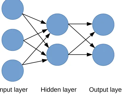
perceptron output of one layer is connected to each perceptron of the next layer. A MLP is composed of an input layer, and output layer and a series of intermediate layers calledhidden layers. Each layer is composed of one or several perceptron units. During the training of a MLP, the weights of the network are tuned in order to minimize the loss function.
Input layer Hidden layer Output layer
Fig. 2: Multi Layer Perceptron with 1 hidden layer.
CNN Convolutional Neural Networks is a family of deep Neural Net-works which combines two types of layers calledConvolutional layers and
Pooling layers and has shown good results specially in the field of image
2 4 3 -1 5 8 -2 4 1 3
1 0 1 0 1 0 1 1 0
5 7 2 3 2 4 8 4 3
Input data
Filters
Filtered data
Fig. 3: Convolution operation using 3 filters of size 3.
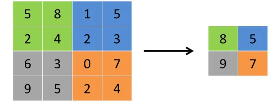
The pooling layers are non-linear layers used to reduce the spatial size of the data. It therefore reduces the amount of computation in the network. It first partitions the input into a set of non-overlapping areas of same dimensions. For each area, the pooling operation outputs a single value which summarizes the input data in this area. The most common types of pooling operations are theMax Pooling operation which outputs the max value of each area and the Average Pooling operation which outputs the average of each area. Fig.4gives an example of Max Pooling operation. The input matrix is divided into non-overlapping areas of size (2×2) and the pooling operation outputs the max values of each area.
5
8
1
5
2
4
2
3
6
3
0
7
9
5
2
4
8
5
9
7
The CNN architecture has a natural translation-invariance property due to the use of pooling operations and shared weights applied across space during the convolution operations. Therefore, CNN is particularly interesting when dealing with de-synchronized side-channel traces as it is able to learn and detect features even if the traces are not perfectly aligned [2].
2.2 Deep Learning in practice
Many open-source Deep Learning frameworks such as Keras [22] or Ten-sorFlow provide user friendly API to build, train and test Deep Learning architectures. For this paper we decided to use Keras and all results pre-sented in the paper were obtained using this framework. After defining the Neural Network architecture the user only needs to provide the training data set and labels to the framework in order to perform the DL training which is managed automatically by the framework.
Loss and Accuracy During a Deep Learning training, it is possible to monitor the loss and accuracy of the training. As introduced in Section 2.1, the loss quantifies the classification error of the network. The accuracy at a given epoch can be defined for instance as the proportion of training samples that are correctly classified by the Neural Network. Both metrics give information about the evolution of the training. A decreasing loss and increasing accuracy usually indicate that the network is properly learning the data, except in case ofoverfitting where the Neural Network actually
memorizes the data instead of learning the targeted features. In the rest
of the paper, we denote asloss∈Rne andacc∈Rne the loss and accuracy
over the epochs of a Deep Learning training, where ne is the number of
epochs used during the training.
Keras offers several options to compute the loss and the accuracy during a Deep Learning training [22]. For the loss function it is for instance possible to use themean squared error or thecategorical crossentropy. For the accuracy one can use for example thecategorical accuracy or the
top-k categorical accuracy. The choice of the loss function can have a big
impact on the learning efficiency. For all results presented in Section 3 and Section 4, we used the mean squared error loss function and the
categorical accuracy as we observed that this combination provided good
results during our experiments.
The validation set is usually a separated set of data which is only used to monitor the training efficiency but is not used for the training itself. It is important that none of the validation samples are part of the training set. When validation samples are used, it is then possible to monitor the validation loss lossval ∈ Rne and validation accuracy accval ∈ Rne over
the epochs which are computed using the validation data. Observing the validation metrics lossval and accval in addition to the metrics loss and acc gives a better overview of the training evolution. If for instance,acc
increases but accval stays stable or decreases, it could mean that
overfit-ting happens and that the network only memorizes the training samples and is not able to classify data outside the training set. On the other hand, if bothaccand accval increase, and both loss and lossval decrease
over the epochs, it indicates that the network learns properly the targeted features and that there is no overfitting.
In the rest of the paper we denote by:
acc, loss=DL(X, Y, ne)
a Deep Learning training over ne epochs, using the set X as training
samples and the set Y as training labels. The accuracy acc ∈ Rne and
loss loss∈Rne of the training are returned as output of this process. In
a similar way, we denote by:
acc, loss, accval, lossval =DL(X, Y, Xval, Yval, ne)
a Deep Learning training using validation samples and labels Xval and Yval, and returns as output the corresponding training and validation
losses and accuracies.
2.3 Profiled Deep Learning Side-Channel attacks
Profiling phase For the profiling phase, a set ofN tracesTk={Ti,k |i=
1, . . . , N}is collected from the profiling device for each key k∈ Kleading to a setX of (N×256) training traces:
X=
255
[
k=0
Tk .
The set of training labels Y is defined as the set of keysz(Ti,k) =k
cor-responding to the training traces. To profile the leakage, a Deep Learn-ing trainLearn-ing DL(X, Y, ne) is performed using the Side-Channel traces as
training data in order to build a Neural Network N able to classify the side-channel traces based on their corresponding key values.
Attack phase To recover the secret key value k∗ ∈ K using M side-channel traces (Ti)16i6M collected from the target device, one first
eval-uates each trace Ti using the trained Neural Network to get M score
vectors yi =N(Ti)∈R|K|. One can then selects the key k which leads to
the highest summed score:
k= argmax
j∈K
M
X
i=1
yi
[j].
The attack is successful if k=k∗.
Interests Previous publications studied the interest of using Deep Learn-ing to perform Profiled Side-Channel attacks. In [1], Maghrebi et al. showed that different type of Neural Networks such as CNN and MLP can outperform other Profiled attacks such as Template Attacks in some cases. In [2], the authors showed that the translation-invariance property of CNN networks can be used against de-synchronized traces to improve the attack results. Moreover, they showed that Data Augmentation can also be applied to artificially increase the size of the training set and im-prove the learning phase and attack results. However, all these studies focused only on applying Deep Learning to perform Profiled attacks.
3 Non-Profiled Deep Learning Side-Channel attacks
3.1 Deep Learning Power Analysis
For the rest of the paper, we consider a Non-Profiled Side-Channel at-tack scenario. In such context, an atat-tacker collects N side-channel traces (Ti)16i6N corresponding to the manipulation of a sensitive valueF(di,k∗)
where (di)16i6N are known random values andk∗∈ K is the fixed secret
value. Usually such an attack is performed following a divide-an-conquer strategy, and one has for instance|K|= 256 withdi and k∗ 8-bit values.
For the rest of the paper we focus on the AES algorithm. In this case, the target function F can be chosen as the AES Sbox function, meaning that F(di,k∗) =Sbox(di⊕k∗).
For a classic Non-Profiled attack such as CPA, for each key hypoth-esis k ∈ K the attacker computes a series of hypothetical intermediate values (Vi,k)16i6N such that Vi,k = F(di, k) and then applies a
leak-age model, for instance the Hamming Weight (HW) leakleak-age model to get series of hypothetical power consumption values (Hi,k)16i6N such
that Hi,k = HW(Vi,k). The attacker then computes the correlation
be-tween the series (Hi,k)16i6N and the collected side-channel traces. For
the correct key value k∗, the series of intermediate values will be cor-rectly guessed, and it will lead to a high correlation if the leakage model is well-chosen. For all the other key candidates, the guessed intermediate values will be wrong and therefore not correlated to the traces, leading to low correlation values. The attacker is able to discriminate the correct key value by selecting the key leading to the highest correlation.
To apply Deep Learning in a Non-Profiled context, our idea is to combine CPA-like hypotheses with Deep Learning trainings. For each key hypothesis k ∈ K the attacker computes the series (Vi,k)16i6N and
(Hi,k)16i6N. He then performs a Deep Learning training using the traces
(Ti)16i6N as training data, and the series (Hi,k)16i6N as the
metrics which can be used is given in Section3.2. We will use the acronym DLPA (Deep Learning Power Analysis) for this new attack method. Al-gorithm 1 summarizes the DLPA procedure to perform a Non-Profiled attack using Deep Learning:
Algorithm 1 DLPA
Inputs: N traces (Ti)16i6N and corresponding plaintexts (di)16i6N. Number of
epochsne.
1: Set training data asX= (Ti)16i6N
2: fork∈ Kdo
3: Compute the series of hypothetical values (Hi,k)16i6N
4: Set training labels asY = (Hi,k)16i6N
5: Perform DL training:acc, loss=DL(X, Y, ne)
6: end for
7: returnkeykwhich leads to the best DL training metrics
It is important to note that the DLPA attack method is not limited to a specific type of Neural Network. In the next section, we study some metrics such as the loss and accuracy which can be used to perform DLPA with any type of Neural Networks. This provides many possibilities when performing the attacks as the attacker can adapt the architecture based on the targeted implementation and device. In this paper, we focus on two variants of DLPA, using MLP and CNN architectures as underlying neural networks. To distinguish both variants, MLP-DLPA will refer to a DLPA process using MLP as Neural Network architecture and CNN-DLPA will refer to a CNN-DLPA attack using CNN.
3.2 Metrics
In this section we study different metrics that can be used to reveal the correct key value during a DLPA attack. To illustrate how the different metrics can lead to the recovery of the secret key, we present some results obtained from a simulation data set. We generatedN = 5,000 simulated traces as follows:
– 50 samples per trace.
– Sbox leakage set at time samplet= 25 and defined asSbox(di⊕k∗) + N(0,1) with di a known randomized byte and k∗ a fixed key byte. N(0,1) corresponds to a Gaussian noise of meanµ= 0 and standard deviationσ= 1.
The purpose of this simulation is only to illustrate how some Deep Learn-ing metrics can be used to discriminate the correct key from the other candidates. More detailed simulations and results are presented in Sec-tion 4. Using this simulation data, we performed the attack as defined in Algorithm 1and observed the following metrics.
Layers weights The first hidden layer of a Multi Layer Perceptron takes as input thensamples of a side-channel trace. By definition of the MLP, each time sample t of the traces is paired with R weights (Wt,j)16j6R
whereRis the number of neurons in the first hidden layer. Therefore, the first hidden layer weights can be seen as a (n×R) matrixW whereWi,j is
the weight of the connection between theith sample of the trace and the
jth neuron of the first hidden layer. Our observations revealed that the Deep Learning process will tend to put higher weights on the time samples corresponding of the side-channel leakage than on the other samples when the correct key is used to compute the labels. To discriminate the correct key guess it is then interesting to observe the following metrics for each time sample tafter the Deep Learning training :
S[t] =
R
X
j=1
(Wt,j)2 (sum of squared weights),
P[t] =
R
Y
j=1
|Wt,j| (product of weights).
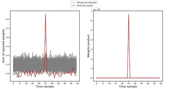
We performed a MLP-DLPA attack as described in Algorithm1using our simulation traces with ne = 50 epochs per guess. The two weights
0 5 10 15 20 25 30 35 40 45 50
Time sample
1.0 1.5 2.0 2.5 3.0 3.5 4.0
Sum of squared weights
0 5 10 15 20 25 30 35 40 45 50
Time sample
0 1 2 3 4 5 6 7
Weights product
1e 50 Wrong key guesses Good key guess
Fig. 5: MLP-DLPA attack using weights metrics. Left: sum of squared weights. Right: product of weights.
We can observe that the correct key guess clearly leads to higher values for the two metrics, at the time sample t= 25 which corresponds to the location of the Sbox leakage. This means that both metrics can be used to reveal the correct key candidate by selecting the key guess leading to the highest values. Additionally, as the highest values are located precisely at
t= 25, this method is also able to reveal the leakage location. Therefore, DLPA using weights metrics can also be used to reveal points of interest (we further discuss this application in Section4.1when targeting masked implementations).
However, such metrics are limited to only specific Neural Network ar-chitectures such as MLP. The following section introduces generic metrics that can be used for any type of Neural Network.
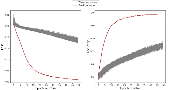
Loss and accuracy As presented in Section 2.2, the two main metrics that can be observed to monitor a Deep Learning training are the loss and the accuracy of the training over the epochs. In this section we show that these two metrics can also be used to discriminate the correct key value when performing a DLPA attack. As illustration, we present in Fig.6the losses and accuracies obtained when performing a MLP-DLPA attack with our simulation data set with ne= 50 epochs per guess. The
by selecting the guess leading to the highest accuracy or lowest loss values. Compared to the weights metrics introduced in the previous section, the loss and accuracy are generic metrics that can be used with any type of Neural Networks.
0 5 10 15 20 25 30 35 40 45 50
Epoch number
0.00 0.05 0.10 0.15 0.20 0.25 0.30
Loss
0 5 10 15 20 25 30 35 40 45 50
Epoch number
0.5 0.6 0.7 0.8 0.9 1.0
Accuracy
Wrong key guesses Good key guess
Fig. 6: Loss (left) and accuracy (right) over the training epochs for all the key guesses when applying DLPA.
Using validation data We observed that using directly loss and accu-racy metrics from the training traces can sometimes lead to poor results. Indeed, in some cases, the neural network is able to lower the loss func-tion and increase the accuracy even for the wrong key candidates. In such cases, it is then interesting to use a set of validation traces as explained in Section2.2and to observe the loss or accuracy obtained from this valida-tion set during the training. The set ofN attack traces can be split into respectively one set of NT training traces, and one set of NV validation
traces withNT+NV =N. Algorithm2summarizes this variant of DLPA
Algorithm 2 DLPA with validation data
Inputs: N traces (Ti)16i6N and corresponding plaintexts (di)16i6N. Number of
epochsne.
1: ChooseNT andNV integers such thatN=NT+NV withNT > NV
2: Set training data asX= (Ti)16i6NT
3: Set validation data asXval= (Ti)NT+16i6N
4: fork∈ Kdo
5: Compute the series of hypothetical values (Hi,k)16i6N
6: Set training labels asY = (Hi,k)16i6NT
7: Set validation labels asYval= (Hi,k)NT+16i6N
8: Perform DL training:acc, loss, accval, lossval=DL(X, Y, Xval, Yval, ne)
9: end for
10: returnkeykwhich leads to the best DL metrics
There is no rule concerning the choice of NT and NV but we usually
wants that NT > NV. It is also important to choose a good trade off
between training and validation data. IfNV is too high, not enough traces
are available for the training. If NV is too low, then the attack may fails
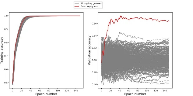
as not enough validation traces are available to reveal the good key value. To simulate conditions where validation data is useful, we generated a set of simulation traces similar as previously, but this time composed of N = 8,000 traces of n= 1,000 points and we added a slight artificial de-synchronization to the traces. We then applied a MLP-DLPA attack with and without validation data with ne = 150 epochs per guess and
compared the results. When using validation data, we split the 8,000 attack traces intoNT = 6,500 training traces andNV = 1,500 validation
0 20 40 60 80 100 120 140
Epoch number
0.5 0.6 0.7 0.8 0.9 1.0
Training accuracy
0 20 40 60 80 100 120 140
Epoch number
0.46 0.48 0.50 0.52 0.54 0.56
Validation accuracy
Wrong key guesses Good key guess
Fig. 7: Comparison of DLPA with and without validation data. Left: Training accuracies with no validation data. Right: Validation accuracies.
We can observe that when no validation data is used, all accuracies tend towards 1 and that it is not possible to distinguish the correct key value. On the other hand, when validation data is used, the validation accuracy reveals the correct key value after a few epochs. It confirms that in some cases it can be useful to use some of the attack traces as validation data and study the corresponding validation metrics to reveal the key.
Summary In this section we presented different metrics which can be used to reveal the correct key value when performing DLPA. Some met-rics, such as the first layer weights of MLP networks are specific to some architectures and some metrics like the loss and accuracy are generic met-rics which can be used with any type of networks. We showed with our examples that all these metrics can be used to reveal the correct key. For the rest of the paper, we decided to use the accuracy as the main metric to determine if the attack is successful. It means that we will consider that a DLPA attack is successful when the training with the good key guess leads to the highest accuracy.
3.3 Labels
Sbox(di ⊕k) as labels for the attack. Indeed, if one uses the identity
labeling Hi,k = Sbox(di ⊕k), the partition of the attack traces derived
from this labeling method will be equivalent for all the key guesses. In other words, the partition of the traces
Pk ={Eu(k) |u∈ {0, . . . ,255}}
defined by the sets
Eu(k)={Ti ∈(Ti)16i6N |Sbox(di⊕k) =u}
is the same for all key guessesk. This means that from one key guess to another, there is no difference in the partition of the attack traces, and that only the labels are permuted which does not impact the training metrics. It means that using the identity labelingHi,k =Sbox(di⊕k) will
naturally lead to similar Deep Learning metrics for all the key candidates, making it impossible to discriminate the correct key value. That is why it is necessary to apply a non-injective function to the Sbox output to compute the labels so that the partition of the attack traces is different from one guess to another. We propose hereafter two methods:
Hamming Weight labeling One solution is to use labels based on the Hamming Weight of the guessed value:
Hi,k =HW(Vi,k).
Binary labeling During our experiments, we noticed that using only two labels derived from the guessed values is also a good alternative. We propose two binary labeling methods to perform DLPA based on the Least Significant bit (LSB) and Most Significant bit (MSB) of the guessed value:
Hi,k =
(
0 ifVi,k <127
1 otherwise (MSB labeling),
Hi,k =Vi,k mod 2 (LSB labeling).
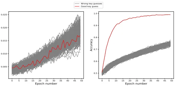
To illustrate the importance of the labeling method, we performed the same attack as in Section 3.2 but using the identity labeling (Hi,k = Sbox(di ⊕k)). The comparison of accuracies obtained when using the
0 5 10 15 20 25 30 35 40 45 50
Epoch number
0.005 0.010 0.015 0.020 0.025
Accuracy
0 5 10 15 20 25 30 35 40 45 50
Epoch number
0.5 0.6 0.7 0.8 0.9 1.0
Accuracy
Wrong key guesses Good key guess
Fig. 8: MLP-DLPA using two different labeling methods. Left: Identity labeling . Right: Binary labeling (MSB).
As expected, the left graph shows that all key guesses lead to similar accuracies when using the identity labeling. All accuracies are not per-fectly identical even when using the identity labeling as the Deep Learn-ing trainLearn-ing is not a deterministic process. Indeed, the trainLearn-ing always depends on the weights initialization as well as the shuffling of the input data during the different epochs, which explains the slight differences be-tween the accuracies even though the identity labeling is used. However, using the identity labeling will always lead to similar accuracies mak-ing it impossible to distmak-inguish the correct key value. That is why it is necessary to use other labeling methods, such as the Hamming Weight or Binary labeling methods. During our experiments, the binary labeling usually provided better results than using Hamming Weight labels. For the rest of the paper, all the results presented were obtained using the binary labeling.
3.4 High-Order attacks
S=Sbox(d⊕k)⊕m1⊕ · · · ⊕ms
The values m1, . . . , ms are called the masks and S is called the masked
value. Each maskmi is generated as a random value for each execution of
the algorithm, making the leakages uncorrelated to the sensitive values. However, High-Order attacks such as High-Order CPA have been devel-oped to target such implementations [24,25,26,27]. A High-Order attack is usually composed of two steps:
– A pre-processing phase: the leakages of the masks are combined with the leakage of the masked value using combination functions such as the absolute difference or centered product [27].
– The attack phase: a statistical distinguisher, for instance the Pearson’s Correlation is used to extract information from the combined leakages traces.
In the rest of the paper, we focus on two practical cases, where an Sbox operation is protected respectively by 1 and 2 random masks as follows:
S=Sbox(d⊕k)⊕m1 ,
S=Sbox(d⊕k)⊕m1⊕m2.
A high-order attack targeting a 1-mask protected implementation is called
a second order attack, and a third order attack corresponds to a
high-order attack targeting an implementation protected with 2 masks.
Leakages combination For a second order attack, one needs to combine the leakage of the mask m1 with the leakage of the masked Sbox value
Sbox(d⊕k)⊕m1. If the locations of the mask and masked value are known,
then one only needs to combine these two leakage locations together. If the locations of the mask and masked value leakages are unknown, a solution is to combine all the possible couples of points in the trace together. If the traces are of size n, such processing will lead to combined traces of size n×(n2−1). Therefore, for large traces, such processing can become too complex and not practical.
4show that it is possible to break implementations protected with 1 and 2 masks using Deep Learning also in a Non-Profiled context with a rea-sonable number of traces. In comparison with High-Order CPA, DLPA does not requires to combine the leakages prior to the attack. Moreover, we show in Section 4.1 that MLP-DLPA can also be used to highlight areas of interest, for instance masks leakages locations, by studying the MLP weights as introduced in Section 3.2.
3.5 CNN and Data Augmentation
In [2], Cagliet al.highlighted that due to its translation-invariance prop-erty, the CNN architecture is naturally able to extract information even from de-synchronized traces. Additionally, they showed that Data Aug-mentation can also be performed to artificially increase the training set size which can lead to more efficient trainings and better results during the attack.
The results presented in Section4 demonstrate that these properties are also applicable when performing DLPA attacks in a Non-Profiled con-text: first, our experiments show that CNN-DLPA leads to good results against de-synchronized traces due to the translation-invariance property of the CNN architecture. Additionally, the results indicate that Data Aug-mentation can also significantly improve the results of MLP-DLPA and CNN-DLPA attacks. Using these properties, we show in Section 4 that DLPA can outperform CPA when attacking de-synchronized traces.
4 Experiments
In this section we further study the efficiency and interests of the DLPA attack method. We focus on the application of MLP-DLPA against masked implementations and the application of DLPA with Data Augmentation against de-synchronized traces. Additionally we present some compar-isons of DLPA with CPA. We perform these experiments using 3 types of side-channel traces:
– Simulated traces.
– Traces collected from the ChipWhisperer-Lite board [14]. – Traces from the public side-channel database ASCAD [3].
4.1 Simulations
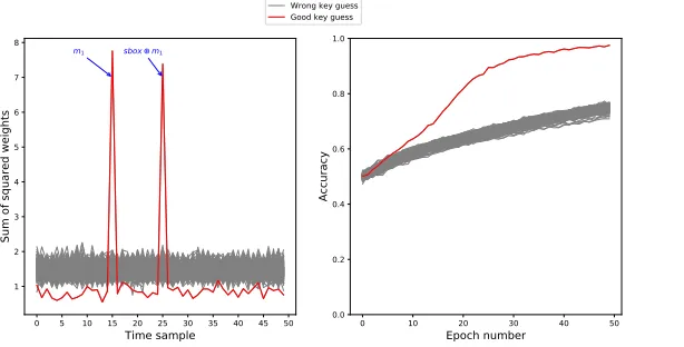
masked implementations. We study the efficiency of MLP-DLPA when targeting an AES Sbox output protected with 1 and 2 random masks. A similar procedure as in Section3.2was used to generate simulated traces. The only difference is that for this experiment, random masks values are added to the simulation traces. To simulate a 1-mask protected Sbox, we generated traces as follows:
– 50 samples per trace.
– Masked Sbox leakage set at t = 25 and defined as Sbox(di ⊕k∗)⊕ m1+N(0,1) with di and m1 randomized bytes and k∗ a fixed key
byte.
– Mask leakage set att= 15 and defined asm1+N(0,1).
– All other points on the traces are chosen as random values in [0; 255].
We applied MLP-DLPA as in Algorithm 1 with ne = 50 epochs per
guess on N = 5,000 simulated traces. In Fig. 9 we present the results of this attack:
0 5 10 15 20 25 30 35 40 45 50
Time sample
1 2 3 4 5 6 7 8
Sum of squared weights
m1 sbox m1
0 10 20 30 40 50
Epoch number
0.0 0.2 0.4 0.6 0.8 1.0
Accuracy
Wrong key guess Good key guess
Fig. 9: MLP-DLPA applied to 1-mask protected Sbox. Left: Sum of squared weights. Right: accuracy over the epochs.
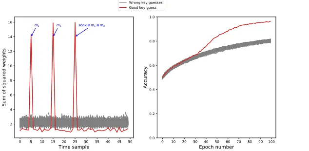
We performed similar experiment on a 2-masks protected Sbox which we simulated as follows:
– 50 samples per trace
– Masked Sbox leakage set at t = 25 and defined as Sbox(di ⊕k∗)⊕ m1⊕m2+N(0,1) with di, m1 and m2 randomized bytes and k∗ a
fixed key byte.
– First mask leakage set att= 15 and defined asm1+N(0,1).
– Second mask leakage set att= 5 and defined asm2+N(0,1).
– All other points on the traces are chosen as random values in [0; 255].
We applied MLP-DLPA withne= 50 epochs per guess onN = 10,000
simulated traces. The results of the attack are presented in Fig. 10.
0 5 10 15 20 25 30 35 40 45 50
Time sample
2 4 6 8 10 12 14 16
Sum of squared weights
m2 m1 sbox m1 m2
0 10 20 30 40 50 60 70 80 90 100
Epoch number
0.0 0.2 0.4 0.6 0.8 1.0
Accuracy
Wrong key guesses Good key guess
Fig. 10: MLP-DLPA applied to 2-masks protected Sbox. Left: Sum of squared weights. Right: accuracy over the epochs.
implementation. DLPA could therefore be combined with other High-Order attacks: for instance the leakages locations revealed by the DLPA could be combined and attacked by a High-Order CPA attack.
CNN-DLPA and Data Augmentation In this section we study the
efficiency of CNN-DLPA with and without Data Augmentation when ap-plied on de-synchronized traces. We simulated unprotected Sbox traces similar as in Section3.2, with only two differences:
– We introduced an artificial jitter in order to simulate de-synchronization. Each trace was shifted left or right by a random value chosen in the interval [−6; 6].
– The noise level was increased toN(0,20) instead ofN(0,1) previously.
We applied 3 attacks onN = 2,000 de-synchronized traces:
– A CPA attack, in order to evaluate the efficiency of a classic Non-Profiled attack against these de-synchronized traces. This will be our reference.
– A CNN-DLPA attack without Data Augmentation. – A CNN-DLPA attack with Data Augmentation.
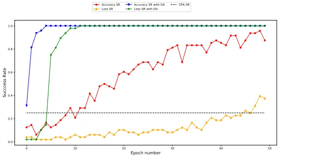
For the third attack we performed Data Augmentation using a method similar to theShifting Deformationpresented in [2]. We decided to fix the Data Augmentation factor to 10, meaning that after DA, the training set to perform the attack is composed ofN0 = 2,000×10 = 20,000 traces. We performed each attack 50 times, each time with a new set of simulated traces, and studied the success rate of these attacks. The CNN-DLPA attacks were performed as in Algorithm1, withne= 50 epochs per guess.
0 10 20 30 40 50
Epoch number
0.0 0.2 0.4 0.6 0.8 1.0
Succcess Rate
Accuracy SR
Loss SR Accuracy SR with DALoss SR with DA CPA SR
Fig. 11: Comparison of success rates between CNN-DLPA (with and with-out DA) and CPA against de-synchronized traces.
We observe that due to the de-synchronization of the Sbox leakage, the CPA only leads to a success rate of around 0.25. Without Data Aug-mentation, we can observe that CNN-DLPA leads to better results, spe-cially when the accuracy metric is used. This is due to the translation-invariance property of the CNN architecture which compensates the effect of the traces de-synchronization. Moreover, when Data Augmentation is applied, the results are clearly improved, leading to success rates of 1 after only a few epochs per guess.
4.2 ChipWhisperer
We used the ChipWhisperer-Lite board [14] in order to validate the effi-ciency of the DLPA method when applied on non-simulated traces with different levels of protections. First, we targeted an unprotected Sbox op-eration with and without de-synchronization. We studied the efficiency of an MLP-DLPA attack in this context, with and without Data Augmen-tation in comparison with a classic CPA attack. Then, we targeted two masked Sbox implementations protected respectively with 1 and 2 masks.
Implementations We implemented an AES Sbox operation Sbox(di⊕
k∗) in C. For the masked implementations, we used a masked re-computed Sbox as described in [23], meaning that the Sbox value Sbox(di⊕k∗) is
never manipulated in plain. For the 1-mask protected implementation, we collected traces containing the execution of the following operations:
– Copy of the maskm1 in memory.
– Copy ofs=Sbox(d⊕k∗)⊕m1 in memory.
Similarly, for the 2-masks protected implementation, we collected traces containing the execution of the following operations:
– Copy of the maskm1 in memory.
– Copy of the maskm2 in memory.
– Copy ofs=Sbox(d⊕k∗)⊕m1⊕m2 in memory.
For the tests against the unprotected implementation, we simply col-lected traces of the copy of s= Sbox(d⊕k∗) in memory. For the three implementations, we fixed a window of 500 points containing only the targeted operations. For the 1 and 2 masks protected implementation, a first order CPA was applied in order to validate that the implementations does not have first order leakages. Moreover, for the 2-masks protected implementation, we also performed a second order CPA attack to verify that the implementation does not have second order leakages.
0 50 100 150 200 250 300 350 400 450 500
Time sample
0.0 0.1 0.2 0.3 0.4 0.5 0.6 0.7
Correlation
0 5 10 15 20 25 30 35 40 45 50
Epoch number
0.5 0.6 0.7 0.8 0.9
Accuracy
Wrong key guesses Good key guess
Fig. 12: Attack on CW unprotected implementation without de-synchronization. Left: First-Order CPA. Right: MLP-DLPA.
As expected, the CPA attack is successful as the targeted implemen-tation is unprotected. We can observe that the DLPA attack is also suc-cessful with only 3,000 traces which shows that the attack is feasible with a very reasonable number of traces even on non-simulated traces.
Unprotected implementation with de-synchronization As the Chip-Whisperer traces are by default almost perfectly synchronized, it is nec-essary to add artificial de-synchronization in order to study the efficiency of DLPA against synchronized traces. We decided to add artificial de-synchronization after the collection of the traces by shifting each trace left or right by a random number of points chosen in the interval [−15; 15]. We applied this software de-synchronization to the 3,000 traces from the previous experiment. We then performed three attacks against these
N = 3,000 de-synchronized traces:
– A first order CPA attack
– A MLP-DLPA attack without Data Augmentation – A MLP-DLPA attack with Data Augmentation
ne = 50 epochs per guess. The results of the 3 attacks are presented in
Fig. 13.
0 50 100 150 200 250 300 350 400 450 500
Time sample
0.000 0.025 0.050 0.075 0.100 0.125 0.150 0.175 0.200
Correlation
0 5 10 15 20 25 30 35 40 45 50
Epoch number
0.48 0.50 0.52 0.54 0.56
Accuracy
0 5 10 15 20 25 30 35 40 45 50
Epoch number
0.500 0.525 0.550 0.575 0.600 0.625 0.650 0.675
Accuracy
Wrong key guesses Good key guess
Fig. 13: Attack on CW unprotected implementation with de-synchronization. Left: CPA. Center: MLP-DLPA without DA. Right: MLP-DLPA with DA.
We can observe that even though the implementation is not protected, the CPA is not successful due to the de-synchronization of the traces. Similarly, the MLP-DLPA attack without Data Augmentation fails to reveal the correct key value. However, we can observe that when using Data Augmentation, the MLP-DLPA is successful and reveals the correct key after a few epochs per guess. It further confirms our results from simulation and shows that Data Augmentation can significantly improve the results of DLPA attacks in a Non-Profiled context using a very limited number of collected traces. Additionally, it also demonstrates that using Data Augmentation should not be limited to the CNN architecture, but can also be used successfully with MLP networks.
Masked implementations We then applied MLP-DLPA attacks against the 1 and 2 masks protected implementations. For the 1-mask protected implementation, we performed the attack on N = 5,000 traces collected from the ChipWhisperer with ne = 150 epochs per guess. As mentioned
0 50 100 150 200 250 300 350 400 450 500
Time sample
0.0 0.1 0.2 0.3 0.4 0.5
Correlation
0 10 20 30 40 50 60 70 80 90 100 110 120 130 140 150
Epoch number
0.5 0.6 0.7 0.8 0.9 1.0
Accuracy
Wrong key guesses Good key guess
Fig. 14: Attack on CW 1-mask protected implementation. Left: First-Order CPA. Right: MLP-DLPA.
As expected, the first order CPA result confirms that the implemen-tation does not have first order leakages. We can observe that the MLP-DLPA attack is successful and reveals the correct key value after only a few epoch per guess. It demonstrates that DLPA can break masked implementations using very reasonable number of traces collected from a device.
We then targeted the 2-masks protected Sbox implementation. We performed a first order and a second order CPA attack on the traces to validate that the implementation does not have first or second order leakages. The first order attack led to results similar to the left graph of Fig. 14 confirming that the implementation does not have first order leakages. To reduce the complexity of the second order attack and of the DLPA, we limited the number of points to 150 points per trace containing the leakages of the two masks as well as the leakage of the masked Sbox. We then combined all the possible couple points from this window using the absolute difference combination function leading to combined traces of size 150×2149 = 11,175 samples. We then performed a second order attack on these combined traces. The MLP-DLPA attack was performed without pre-processing, directly on the raw traces of 150 points with
ne = 100 epochs per guess. Both attacks were performed using 50,000
0 2000 4000 6000 8000 10000
Time sample
0.0 0.1 0.2 0.3 0.4 0.5
Correlation
0 10 20 30 40 50 60 70 80 90 100
Epoch number
0.500 0.525 0.550 0.575 0.600 0.625 0.650 0.675
Accuracy
Wrong key guesses Good key guess
Fig. 15: Attack on CW 2-masks protected implementation. Left: Second-Order CPA. Right: MLP-DLPA.
It can be observed that the MLP-DLPA attack reveals the correct key value after around 50 epochs per guess. On the other hand, the second order CPA is not successful. The result of the second order CPA applied on 50,000 traces from the ChipWhisperer gives a high level of confidence that the implementation does not have second order leakages. This shows that the MLP-DLPA method is able to combine the leakages of 3 differ-ent shares to reveal the secret key, even on non-simulated data, with a reasonable number of traces and without traces pre-processing.
4.3 ASCAD
ASCAD is a public database recently introduced by Prouff et al. in [3] to provide a common set of side-channel traces for research on Deep Learning-based Side-Channel attacks. The targeted implementation is a first order protected Software AES implementation running on an 8-bit ATMega8515 board. The main database ASCAD.h5 is composed of two set of traces: a profiling set of 50,000 traces to train Deep Learning ar-chitectures and an attack set of 10,000 traces to test the efficiency of the trained Neural Networks. Each trace of the database is composed of 700 samples focusing on the processing of the third byte of the masked state
and attack sets of the ASCAD database. In this section, we validate our Non-Profiled Deep Learning attack using this public database.
For both the profiling set and the attack set of ASCAD.h5, the same 16-byte fixed key is used while the plaintexts and masks are randomized. Therefore, as the key is always fixed, both the attack set and profiling set can be considered as traces obtained from a closed device to perform a Non-Profiled attack. We decided to use the profiling set to perform our experiment as it contains more traces than the attack set. We applied a MLP-DLPA attack on the first 20,000 traces of the profiling set of ASCAD.h5 with ne = 50 epochs per guess. The result of this attack is
presented in Fig. 16.
0 5 10 15 20 25 30 35 40 45 50
Epoch number
0.500 0.525 0.550 0.575 0.600 0.625 0.650 0.675
Accuracy
Wrong key guesses Good key guess
Fig. 16: MLP-DLPA attack on ASCAD.
The results show a clear success of the attack with 20,000 traces from theASCAD.h5database. It further confirms the validity of the method as well as its interest. The execution times of this attack and of previous attacks are given in the next section.
4.4 Complexity
DLPA will be slower than first order CPA, due to the multiple train-ings needed for DLPA. However, for high order attacks, we showed that DLPA does not require to combine leakage points together before the at-tack. As an example, to perform a second order attack on the ASCAD traces, as the location of the leakages are unknown, one would need to perform a leakage combination on 700 points for each trace. This means that a total 700×2699 = 244,650 points per traces must be processed dur-ing pre-processdur-ing and durdur-ing the attack phase which would lead to a high complexity. On the other hand, DLPA does not requires any pre-processing and it able to reveal the secret key after only a few epochs. If we limit our attack on ASCAD to only 5 epochs per guess, the attack only requires around 10 minutes on our setup and is still successful. For comparison, we performed a second order CPA on the ASCAD traces by combining all the 244,650 couples of point for each trace. The execution times of this CPA attack and of different DLPA attacks are summarized in Table. 1. We recorded these values when running the attacks in Python on our personal computer with 32 GB of RAM, a GeForce GTX 1080 GPU and a Intel Xeon E5-2687W CPU.
Implementation Attack Nb traces Nb samples Nb epochs Time (hours)
CW 1-mask MLP-DLPA 5,000 500 150 0.92
CW 2-masks MLP-DLPA 50,000 150 100 5.14
ASCAD MLP-DLPA 20,000 700 50 1.19
ASCAD MLP-DLPA 20,000 700 5 0.17
ASCAD 2nd order CPA 1,000 700 N/A 2.16
Table 1: Execution times comparison.
DLPA. This further confirms that DLPA can be an interesting alternative for instance when performing Non-Profiled High-Order attacks.
5 Conclusion
In this paper we introduced a new attack method to apply Deep Learn-ing techniques in a Non-Profiled context. We showed that it is possible to use Deep Learning and Neural Networks even when attacking a closed device where no profiling is possible. The possibility to use Deep Learning for Non-Profiled attacks offers several benefits: we showed that even in a Non-Profiled context, the translation-invariance property of Convolu-tional Neural Networks can be exploited against de-synchronized traces and that it is possible to perform Data Augmentation with MLP and CNN architectures to improve the results of Non-Profiled attacks. Using these properties, we obtained results where Non-Profiled Deep Learning-based attacks can outperform classic Non-Profiled attacks as CPA. This new attack method can also be applied to break high-order protected im-plementation, without applying any leakage combination pre-processing. The complexity snapshot that we provide, shows that this attack method is practical and may even be more efficient than some existing attacks in some cases, for instance when attacking masked implementations. Fi-nally, this attack can be implemented in a few lines of code using Deep Learning frameworks such as Keras.
References
1. H. Maghrebi, T. Portigliatti, and E. Prouff, “Breaking cryptographic imple-mentations using deep learning techniques.” Cryptology ePrint Archive, Report
2016/921, 2016. https://eprint.iacr.org/2016/921.
2. E. Cagli, C. Dumas, and E. Prouff, Convolutional Neural Networks with Data
Augmentation Against Jitter-Based Countermeasures, pp. 45–68. Cham: Springer International Publishing, 2017.
3. Emmanuel Prouff and Remi Strullu and Ryad Benadjila and Eleonora Cagli and Cecile Dumas, “Study of Deep Learning Techniques for Side-Channel Analysis and Introduction to ASCAD Database.” Cryptology ePrint Archive, Report 2018/053,
2018. https://eprint.iacr.org/2018/053.
4. P. C. Kocher, “Timing Attacks on Implementations of Diffie-Hellman, RSA, DSS,
and Other Systems.,” inAdvances in Cryptology - CRYPTO ’96(N. Koblitz, ed.),
vol. 1109 ofLecture Notes in Computer Science, pp. 104–113, Springer, 1996.
5. S. Chari, J. R. Rao, and P. Rohatgi,Template Attacks, pp. 13–28. Berlin,
Heidel-berg: Springer Berlin Heidelberg, 2003.
6. J. Doget, E. Prouff, M. Rivain, and F.-X. Standaert, “Univariate side channel
at-tacks and leakage modeling,”Journal of Cryptographic Engineering, vol. 1, p. 123,
7. W. Schindler, K. Lemke, and C. Paar, “A stochastic model for differential side
channel cryptanalysis,” inCryptographic Hardware and Embedded Systems – CHES
2005 (J. R. Rao and B. Sunar, eds.), (Berlin, Heidelberg), pp. 30–46, Springer
Berlin Heidelberg, 2005.
8. G. Hospodar, B. Gierlichs, E. De Mulder, I. Verbauwhede, and J. Vandewalle,
“Machine learning in side-channel analysis: a first study,”Journal of Cryptographic
Engineering, vol. 1, p. 293, Oct 2011.
9. L. Lerman, R. Poussier, G. Bontempi, O. Markowitch, and F.-X. Standaert, “Tem-plate attacks vs. machine learning revisited and the curse of dimensionality in
side-channel analysis,” inRevised Selected Papers of the 6th International Workshop on
Constructive Side-Channel Analysis and Secure Design - Volume 9064, COSADE 2015, (New York, NY, USA), pp. 20–33, Springer-Verlag New York, Inc., 2015. 10. L. Lerman, G. Bontempi, and O. Markowitch, “A machine learning approach
against a masked aes,”Journal of Cryptographic Engineering, vol. 5, pp. 123–139,
Jun 2015.
11. P. C. Kocher, J. Jaffe, and B. Jun, “Differential Power Analysis,” in Advances
in Cryptology - CRYPTO ’99(M. J. Wiener, ed.), vol. 1666 of Lecture Notes in Computer Science, pp. 388–397, Springer, 1999.
12. E. Brier, C. Clavier, and F. Olivier, “Correlation Power Analysis with a Leakage
Model,” inCHES, pp. 16–29, 2004.
13. B. Gierlichs, L. Batina, P. Tuyls, and B. Preneel, Mutual Information Analysis,
pp. 426–442. Berlin, Heidelberg: Springer Berlin Heidelberg, 2008.
14. “ChipWhisperer Website.”https://newae.com/tools/chipwhisperer/.
15. C. M. Bishop, Pattern Recognition and Machine Learning (Information Science
and Statistics). Secaucus, NJ, USA: Springer-Verlag New York, Inc., 2006.
16. Y. LeCun, Y. Bengio, and G. E. Hinton, “Deep learning,” Nature, vol. 521,
no. 7553, pp. 436–444, 2015.
17. “Deep Learning website.”http://deeplearning.net/tutorial/tutorial.
18. I. Goodfellow, Y. Bengio, and A. Courville, Deep Learning. MIT Press, 2016.
http://www.deeplearningbook.org.
19. C. M. Bishop, Neural Networks for Pattern Recognition. New York, NY, USA:
Oxford University Press, Inc., 1995.
20. Y. Lecun and Y. Bengio, Convolutional networks for images, speech, and
time-series. MIT Press, 1995.
21. K. O’Shea and R. Nash, “An introduction to convolutional neural networks,” 11 2015.
22. “Keras framework.”http://www.keras.io.
23. M.-L. Akkar and C. Giraud, “An Implementation of DES and AES, Secure against
Some Attacks,” in CHES (C¸ etin Kaya Ko¸c, D. Naccache, and C. Paar, eds.),
vol. 2162 ofLecture Notes in Computer Science, pp. 309–318, Springer, 2001.
24. T. S. Messerges, “Using Second-Order Power Analysis to Attack DPA Resistant Software,” pp. 238–251.
25. M. Joye, P. Paillier, and B. Schoenmakers, “On Second-Order Differential Power
Analysis.,” inCryptographic Hardware and Embedded Systems - CHES 2005(J. R.
Rao and B. Sunar, eds.), vol. 3659 ofLecture Notes in Computer Science, pp. 293–
308, Springer, 2005.
26. J. Waddle and D. Wagner, “Towards Efficient Second-Order Power Analysis,” in
CHES, pp. 1–15, 2004.
27. E. Prouff, M. Rivain, and R. Bevan, “Statistical Analysis of Second Order
Differ-ential Power Analysis,”IEEE Transactions on Computers, vol. 58, pp. 799–811,