On the Application of Massive MIMO Systems to Machine Type Communications

(1)

1

On the Application of Massive MIMO Systems to

Machine Type Communications

Felipe A. P. de Figueiredo

∗

, Fabbryccio A. C. M. Cardoso

†

, Ingrid Moerman

∗

and Gustavo Fraidenraich

‡ ∗

_{Ghent University - imec, IDLab, Department of Information Technology, Ghent, Belgium.}

†

_{CPqD – Research and Development Center on Telecommunications, Brazil.}

‡

_{DECOM/FEEC – State University of Campinas (UNICAMP), Brazil.}

Email:

∗

[felipe.pereira, ingrid.moerman]@ugent.be,

†

Abstract—This paper evaluates the feasibility of applying Mas-sive MIMO to tackle the uplink mixed-service communication problem. Under the assumption of an available physical narrow-band shared channel (PNSCH), devised to exclusively consume data traffic from Machine Type Communications (MTC) devices, the capacity (i.e., number of connected devices) of MTC networks and, in turn, that of the whole system, can be increased by clustering such devices and letting each cluster share the same time-frequency physical resource blocks. Following this research line, we study the possibility of employing sub-optimal linear detectors to the problem and present a simple and practical channel estimator that works without previous knowledge of the large-scale channel coefficients. Our simulation results suggest that the proposed channel estimator performs asymptotically as well as the MMSE estimator with respect to the number of antennas and the uplink transmission power. Furthermore, the results also indicate that, as the number of antennas is made progressively larger, the performance of sub-optimal linear de-tection methods approaches the perfect interference-cancellation bound. The findings presented in this paper shed light on and motivate for new and exciting research lines towards a better understanding of the use of massive MIMO in MTC networks.

Index Terms—Large-scale antenna systems, 5G networks, ma-chine type communications, channel estimation, linear detection.

I. INTRODUCTION

R

ECENT technological developments taking place in our society have been drastically changing the way we use communications systems. These changes are in their great part due to the huge (and also foreseen [1]) increase in on-demand data consumption over both wireless and mobile networks. In order to support such changes, it is mandatory to devise solutions that can meet the different requirements of use cases regarded as the market drivers for next generation wireless networks (5G). ITU-R has defined the following three main 5G use cases: Enhanced Mobile Broadband (eMBB); Ultra-Reliable and Low Latency Communications (URLLC); and Massive Machine Type Communications (mMTC) [2]. They aim at significantly improving performance, scalability and (cost/energy) efficiency of the current wireless networks such as LTE, LTE-A and LTE-A Pro. These use cases and their direct requirements will demand huge improvements in comparison with the previous generation of IMT systems [2]. A non-exhaustive list of 5G applications grouped by use case and a brief explanation about them follows next.

• eMBB: focus on improvements to data rate, user density, latency, capacity and coverage of the current wireless networks [3], [4]. Some applications are: high-speed mobile broadband, augmented and virtual realities (e.g., gaming), smart office environments, pervasive video (i.e., high-resolution video everywhere), etc.

• URLLC: aims at allowing devices and machines to communicate with ultra-reliability, high availability and very low latency, which make it ideal for real-time applications [5]–[7]. Some applications are: wireless industrial control, factory automation, remote surgery, cellular vehicle-to-everything (C-V2X) communications, self-driving cars, smart grids, public safety, etc.

• mMTC: focus on enabling machine-centered commu-nications among devices that are massive in number, battery-driven, generate bursty traffic and have low-cost, i.e., Internet of Things (IoT) devices [3], [8], [9]. This use case is intended to support applications like: smart metering, smart cities, asset tracking, remote monitoring (e.g., field and body sensors), etc.

Applications within the scope of the MTC driver range from smart cities and smart grid to critical infrastructure monitoring [10]–[12], and from Advanced Driver Assistance Systems (ADAS) to mobile health, which includes sports/fitness and telemedicine [13], [14]. Reliability in critical infrastructure monitoring and smart grid, for example, is often achieved only through dedicated land-line connections (i.e., wired connec-tions) [15]–[17]. Telemedicine makes use of telecommunica-tions and information technology systems in order to provide remote clinical health care. It involves, for example, diag-nostics realized through medical data stored in cloud servers, which requires low-latency, real-time access and high capacity servers capable of dealing with massive amounts of data,e.g., computerized axial tomography and magnetic resonance imag-ing [18]–[20]. Automotive infotainment, vehicular cooperation in ADAS, and pre-crash sensing and mitigation applications also require high-speed, low-latency car-to-infrastructure and car-to-car communications [21]–[23].

Reliability and power consumption are of huge importance for wireless sensor networks (WSN), where a few to several hundreds or even thousands of low-cost and power-constrained sensor devices (in most of the WSNs, the sensors are battery-powered) need to measure environmental conditions like

tem-Preprints (www.preprints.org) | NOT PEER-REVIEWED | Posted: 10 December 2018

Preprints (www.preprints.org) | NOT PEER-REVIEWED | Posted: 10 December 2018 doi:10.20944/preprints201812.0100.v1

(2)

2

perature, noise level, air pollution levels, humidity, wind, etc. and reliably transmit them to a central location over harsh channel conditions [24], [25]. Most of the WSN use cases require the deployment of battery-powered sensors for ten years without any maintenance, meaning that the battery is expected to last a decade without being recharged [26].

As can be noticed from the previous discussion, the require-ments necessary for the implementation of next generation wireless networks (i.e., 5G) are quite diverse, even within the same market driver. Scalability is yet another issue posed by IoT, as the main assumption behind it is that hundreds to hundreds of thousands of low-cost MTC devices shall be served by a single Base Station (BS) [27]. Scalability issues have been mainly tackled by adopting different and sometimes complementary approaches, such as sparse signal processing techniques [28], techniques brought from duty-cycled Wireless Sensor Networks [29] and new waveforms specially designed for bursty and asynchronous data transmissions [30], [31], however, until now, the use of Multiple Input Multiple Output (MIMO) techniques in the context of MTC networks and the scalability issue are less understood.

The sentiment shared by most researchers nowadays is that the foreseen increase in data rate will be achieved by

combined gains [32] provided by (i) increasing the network density, i.e., the addition of more radio sites with smaller cell coverage areas to the same region (extreme network densification), which consequently improves the area spectral efficiency [33] (ii) increasing spectrum availability such as the introduction of new spectrum bands like mmWaves [34], [35], (iii) improving the use of licensed, unlicensed and licensed-shared spectrum bands [36] with more efficient and intelligent sharing techniques, (iv) and increasing spectral efficiency of digital communications systems through advances in MIMO techniques. One of the benefits resulting directly from the powerful processing gains provided by the use of large arrays of antennas (i.e., massive MIMO systems) is that the majority of the physical layer signal processing and and resource allocation (i.e., scheduling) issues are simplified, if not solved, which is clearly not the case for systems employing only a moderate to small number of antennas [37].

Massive MIMO has been gaining significant attention and strength as a very promising candidate to improve spectral efficiency and consequently increase the channel capacity in multi-user networks. Massive MIMO is a scalable technol-ogy through which large numbers of devices can simulta-neously communicate through the entire allocated spectrum, i.e., thanks to its many spatial degrees of freedom, the same allocated frequency band can be reused by many users at the same time [37]. In the limit, as the number of antennas, M, deployed at the BS increases, the system processing gain also increases, i.e., as M tends to infinity, the processing gain tends to infinity as well. Massive MIMO not only provides high spectral efficiency in a cell, but also provides a good and uniform service to a large number of devices simultaneously [37]. A consequence of this powerful processing gain is that the effects of small-scale fading and frequency dependence disappear. In [38] it is indicated that, due to the law of large numbers, the channel becomes reliable (i.e., it becomes

deterministic) so that each one of the subcarriers in an OFDM-based massive MIMO system considerably experiences the same channel gain. This phenomenon is known as channel hardening[39].Channel hardeningrenders frequency-domain scheduling unnecessary as all subcarriers are considered equally good, and consequently, makes most of the physical layer control signaling no longer needed [40]. Additionally, the adoption of massive MIMO systems also improve frequency reuse (due to the reduced radiated power), simplifies power control (power control coefficients depend only on the large-scale fading coefficients) and decreases multi-user interference (due to the possibility of having very narrow beams as M increases) [39], [41].

On the other hand, massive MIMO also presents some challenges that need to be studied and addressed in order to fully reap its benefits. Next, some of the issues regarded as the most challenging in the Massive MIMO literature are briefly discussed.

• In multi-cell scenarios, the use of non-orthogonal pilot signals by different users in different cells during the training-phase brings about a phenomenon known as

pilot-contamination, which makes the target user’s chan-nel estimate contaminated by other user’s chanchan-nels using the same pilot. This phenomenon degrades the quality of the channel estimates and causes coherent interference that does not vanish by increasing the number of antennas [38], [42].

• Cost-efficient massive MIMO systems are expected to be constructed making use of low-cost components, however, this leads to the appearance of non-negligible signal distortion caused by hardware impairments. Hard-ware impairments cause channel estimation errors and limit the system’s achievable capacity, which theoretically should be unlimited as the number of antennas increases, due to phase-noise, I/Q imbalance, power-amplifier non-linearities, and quantization errors generally intrinsic to low-cost components [43].

• The digital signal processing in massive MIMO systems is inherently more computationally challenging when compared to the processing required by systems with single or small number of antennas. The signal pro-cessing in massive MIMO systems generally involves the following tasks: fast Fourier transform (FFT), chan-nel estimation, precoding/detection and computation of precoding/detection matrices. The complexity of these digital signal processing operations increases linearly with the number of antennas, and everything but the FFT processing complexity also scales with the number of de-vices. Therefore, low-complexity digital signal processing techniques have to be devised in order to deal with this massive computational complexity expected to be created by these systems [38], [40].

(3)

3

TABLE I

BENEFITS ANDCHALLENGES OFMASSIVEMIMOSYSTEMS

Characteristic Explanation References

Benefits

High spectrum efficiency Huge multiplexing and array gains [38], [41], [49] High energy efficiency Concentration of radiated energy on specific UEs [41]

High reliability Increased diversity gain [41], [49]

Efficient linear precoding and detection Favorable propagation condition for i.i.d. Rayleigh channels [39], [41] Weak inter-user interference and With largeM, channels become orthogonal and with extremely [41], [43] enhanced physical layer security narrow beams

Simpler scheduling scheme Channel hardening effect averages out fast fading and receiver noise [40], [41], [50] Robustness to failures of individual Massive number of antenna elements [38], [41] antenna elements

Challenges

Pilot-contamination Limited number of orthogonal pilots due to coherence interval [38], [42] Hardware impairments Cost-efficient massive MIMO deployments use low-cost components, [43]

which suffer from hardware impairments

High digital signal processing complexity Digital signal processing scales with number of antennas and devices [38], [40] Non-reciprocal transceiver characteristics Transfer response of RF transceiver chains (amplifiers, filters, etc.) are different [44]

a time interval. Based on the reciprocity assumption, TDD massive MIMO systems use the uplink channel as an estimate of the downlink channel. However, an issue that arises from this approach is that the transfer charac-teristics of transmit and receive RF (i.e., RF transceiver) chains are different (amplifiers, filters, local oscillators, etc. have different characteristics), which directly impacts the calculation of precoding matrices. Therefore, effective and efficient reciprocity calibration techniques are needed to exploit the channel reciprocity in practice [44]. Although the deployment of massive MIMO systems still poses several challenges (i.e., open questions), theoretical and measurement results demonstrate that its adoption can tremendously improve the spectral efficiency of wireless com-munications systems, [39], [41]. In Table I we summarize the most important benefits and challenges brought about by massive MIMO technologies.

The adoption of massive MIMO technology can specially help leveraging and simplifying the deployment of mMTC systems in cellular networks, which are potential candidates to accommodate the emerging MTC data traffic thanks to the existing infrastructure and wide-area coverage [45]. Massive MIMO has the potential to enable the multiplexing of a myriad of devices in the same time/frequency resources along with an extension in range due to the coherent beamforming gain inherent to this technology [37], [45].

The main contribution of this paper is the proposal of a data transmission scheme employing massive MIMO technology as a way to address the uplink mixed-service communication problem. In the uplink mixed-service communication problem, a BS has to serve not only Human Type Communications (HTC) devices but also a possible massive number of MTC devices. In order to be addressed properly, the problem can be split into two subproblems, namely, random access and data transmission problems. During the random access phase, a huge number of MTC along with HTC devices might simulta-neously try access the network, which results in congestion and overloading [46]. On the other hand, after the MTC devices are granted access to the network, the BS has to allocate dedicated physical resource blocks to these devices [47]. With the foreseen number of connected devices raising up to tens of

thousands per cell [46], a BS might easily run out of available physical resource blocks (i.e., congestion due to user data packets) to accommodate the data transmissions of this huge number of devices, tremendously impacting on the operations and quality of the provided services of a mobile network.

We focus our work on the data transmission phase by proposing a massive MIMO-based scheme where the data transmissions of a great number of MTC devices are served through the same time-frequency resources by a BS equipped with a large number of antennas. The proposed scheme has the potential to mitigate the congestion due to the large (and pos-sibly massive) number of user data packets and additionally, it offers scalability, as the number of served devices can easily grow by increasing the number of deployed antennas at the BS [37]. The proposed scheme deals with data transmission, channel estimation and detection of the many data streams simultaneously transmitted by multiple MTC devices using the PNSCH’s shared time-frequency resources.

We employ the maximum likelihood (ML) method to find an estimator for the large-scale fading coefficients present in the MMSE channel estimator. We show that this estimator is not only unbiased but it also achieves the Cr´amer-Rao lower bound. The estimated large-scale fading coefficients are replaced into the MMSE channel estimator, giving rise to a new channel estimator, which asymptotically approaches the performance of the MMSE channel estimator as the number of antennas and the uplink transmit power increase. Additionally, we derive closed-form and approximate expressions for the mean square error (MSE) of the proposed estimator. Moreover, we find lower bounds on the achievable rate for each one of the studied linear detectors. We also show that even for simple linear receivers (i.e., MRC, ZF and MMSE), the transmitted power of each MTC device can be reduced as the number of antennas, M, grows without bound, which is very beneficial for power-constrained devices running on batteries.

This paper is an extension of a previous paper [48]. Differ-ently from [48], where we have only considered Bit Error Rate (BER) analysis for perfect channel estimation (i.e., full chan-nel knowledge) and some linear detectors, the current paper not only deals with imperfect channel estimation, proposing and assessing the performance of a channel estimator in terms

Preprints (www.preprints.org) | NOT PEER-REVIEWED | Posted: 10 December 2018

(4)

4

of mean squared error (MSE) and BER, but also proposes a scheme to tackle the problem posed by the simultaneous data transmission of a large number of MTC devices connected to the base station (i.e., user data packet congestion). Addition-ally, we also analyze the achievable rates of the studied linear detectors with the proposed data transmission scheme.

The remainder of the paper is as follows. Section II provides a brief discussion on related works. Section III presents a study case, where the feasibility of Massive MIMO for MTC networks is investigated as means to address the uplink mixed-service communication problem. Section IV outlines one pos-sible approach to estimate the large-scale fading coefficients. Section V proposes a channel estimator that takes into account the estimation of the large-scale fading coefficients. Section VI presents simulation results and discussions on the outcomes. Section VII wraps up the paper with concluding remarks.

A. Notations

Vectors and matrices are denoted by bold lower-case and upper-case letters, respectively. The matrix/vector conjugate-transpose is denoted by(.)H_{. We use}

E[.], var(.)and Cov[.]

to denote the expectation, variance and covariance operators. The circularly-symmetric Gaussian distribution is denoted by CN. We denote equality in asymptotic sense by≈a. Γ(.)and B(., .) denote the Gamma and Beta functions respectively.

IK is the K×K identity matrix and 0N is the N ×1 zero

vector. k.k,P{.},R{.} andcos−1(.)denote Euclidean norm,

probability, real part and arc-cosine respectively. The big-O notationO(M x)describes that the complexity is bounded by CM x for some 0< C <∞.

II. RELATEDWORK

In the literature, there are a myriad of works proposing solutions exclusively tailored to increase the capacity of the random access channel of LTE/LTE-A networks. In those networks, the MTC devices compete for resource blocks for their data transmission using a random access scheme. The works [46], [51]–[54] and the vast number of papers IWT’2015

Application Context

Narrowband MTC Devices

Wideband application

Device 1

Front End

⋮ Device 2

Device K

⋮

#1

#2

# #1

#2

#

ℎ ⋯ ℎ

⋮ ⋱ ⋮

ℎ ⋯ ℎ

MMIMO Channel

UE

Front End

⋮

#1

#

MIMO ×

ℎ ⋯ ℎ

⋮ ⋱ ⋮

ℎ ⋯ ℎ

MIMO Channel

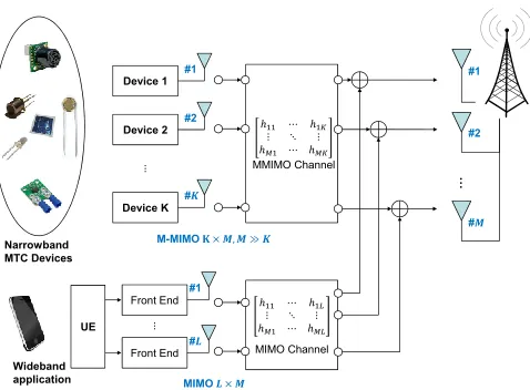
How to enable thousands of low rate devices in a cell without compromising the RAN ?

M-MIMO × , ≫

Fig. 1. Context application: Enabling a great number of low rate MTC devices in a cell.

therein mentioned, review and propose solutions to tackle the scalability issue posed by the random access of tens to hundreds of thousands of MTC devices during the random access/synchronization phase. The solutions presented in these works can accommodate from 30000 to more than 78000 MTC devices per cell with low collision probabilities. However, these works do not deal with the problem involving simul-taneous data transmissions coming from a possible massive number of MTC devices during the Radio Resource Control (RRC) connected state [47].

Although there exist numerous studies on the massive random access problem, there are relatively few publications addressing the massive data transmission problem (i.e., con-gestion due to user data packets) [55], which arises from the simultaneous data transmission of a huge number of devices during the RRC connected state (i.e., during the data transmission phase).

The work presented in [56] tackles the problem of device activity detection and joint channel estimation when non-orthogonal pilot sequences are used by the devices. The authors use approximate message passing (AMP) algorithm in compressed sensing to exploit the sparsity in device activity detection. The work considers a grant-free multiple-access scheme and that the devices are already synchronized to the BS. The drawbacks of the proposed solution are the lack of information on how the devices stay synchronized to the BS and the analysis for multi-cell scenarios. In [57] the authors study the coexistence of HTC and MTC devices under a single-cell massive MIMO setup and assess their joint spectral efficiency, however they do not deal with channel estimation, linear decoding problems and multi-cell scenarios. The authors of [58] develop a stochastic geometry model for dense MTC systems adopting massive MIMO setups however, their focus is on providing a random access solution for such networks, failing to analyze the impact of massive MIMO during the data transmission phase. Additionally, it is worth noticing that all these works assume that all devices are synchronized to the uplink of the base station.

Therefore, we decided to focus our work on the data transmission phase, by proposing a solution where clusters of MTC devices share exclusive and periodic time-frequency resources and simultaneously transmit their data with massive MIMO technology being deployed at the BS to retrieve each one of the device’s transmissions. By using massive MIMO at the BS, a great number of MTC devices can be assigned to the same time-frequency resources, consequently, mitigating the negative effects on human type communications (HTC), e.g., data congestion. The proposed solution allows the addition of MTC services to wireless cellular networks without the necessity of additional time-frequency resources.

III. THEUPLINKMIXED-SERVICECOMMUNICATIONS

PROBLEM

(5)

5

IWT’2015

System Model: Massive MU-MIMO uplink for mixed

device types

CP

⋮

CP

CP IFFT

#1

#2

#𝐾

ℎ₁₁ ⋯ ℎ_1𝐾

⋮ ⋱ ⋮

ℎ_𝑀1 ⋯ ℎ_𝑀𝐾

M M IMO Channel

MMIMO 𝐾 × 𝑀

⋮

#1

#2

#𝑀

CP

CP CP Subcarrier indexes

IFFT

⋮

𝑎₁₁ ⋯ 𝑎_1𝐾

⋮ ⋱ ⋮

𝑎𝑀1 ⋯ 𝑎𝑀𝐾

M M IMO Detector

(Linear Decoding) FFT

FFT

FFT #1

#2

#𝐾 _Subcarrier

Extraction Subcarrier indexes

Subcarrier Extraction Subcarrier Extraction

⋮

෠ℎ11 ⋯ ෠ℎ1𝐾

⋮ ⋱ ⋮

෠ℎ𝑀1 ⋯ ෠ℎ𝑀𝐾

M M IMO Channel

Estimator

⋮

Pilot K Source K

Pilot 2 Source 2

Pilot 1 Source 1

Base Station Matched

Subband Filter Subband Filter

⋮

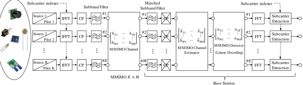
Fig. 2. Block diagram of a Massive MIMO uplink for mixed networks, where the BS simultaneously serves narrowband MTC devices and wideband UEs. The cluster of MTC devices seen at the transmit side share the same time-frequency PRBs, while the sole BS at the receive side is equipped with an antenna array at least one order of magnitude larger than the number of MTC devices.

Fourth Generation (4G) wideband User Equipment (UEs). We propose an approach that enables a huge number of bursty and low rate devices in a cell without compromising the Radio Access Network (RAN) as depicted in Figure 1. Our proposal is in line with the set of MTC features considered in 3GPP [55], [59]: (i) low mobility: the devices rarely move or only move within a certain region; (ii) time controlled: MTC data delivery only occurs during predefined time intervals; (iii) time tolerant: MTC data transfer can be delayed; (iv) small data transmissions: only small amounts of data are exchanged between the device and the BS,i.e., bursty transmissions; (v) mobile originated only: MTC devices utilizing only mobile originated communications; (vi) infrequent transmission: long period between two data transmissions. Treating MTC devices as regular UEs turns out to be an issue, as scheduling Physical Resource Blocks (PRBs) in extremely dense networks is a nontrivial task made harder in the presence of retransmissions and intrinsic uplink synchronization procedures [60]–[63].

Assuming the availability of a Physical Narrowband Shared Channel (PNSCH), exclusively devised to consume data traffic generated by MTC devices, the capacity of the MTC network – and, in turn, that of the mixed-service system – can be increased by clustering MTC devices and letting clusters share the same time-frequency PRBs. The idea behind the PNSCH is to allow the exploitation of the channel’s geometric scattering characteristics to spread MTC signals in the spatial domain. The individual data streams conveyed by spatially spread MTC signals can be separated thanks to the inherent spatial multiplexing properties of massive MIMO technology [39], where the antenna array size at the BS is at least one order of magnitude larger than the number of served MTC devices. Next, we describe the system depicted in Figure 2 in terms of its underlying functional blocks.

A. Signal Generation & Transmission

We assume the transmitted signals of a cluster with K single-antenna MTC devices are detected by a Massive MIMO BS equipped with M receive antennas, M K. All theK MTC sources map data into a set of continuous PRBs in the

frequency domain, with the subcarrier indexes providing the spectral position of the PNSCH at the physical layer level.

As the focus of our work is on the data transmission phase (i.e., during the RRC CONNECTED state [47]), we, therefore, assume that all MTC devices being served by a BS are already synchronized and connected to it before accessing the PNSCH,i.e., the MTC devices have already performed the random access and attach procedures before any data is sent through the PNSCH. Before any transmission, in order to align its uplink transmissions to the BS timing, each one of the MTC devices must perform a random access procedure through the physical random access channel (PRACH) [47], [62], [64]. Upon successful random access procedure, a MTC device holds a Cell-Radio Temporary Identifier (C-RNTI) that is then mapped to a pilot sequence, which will be used uniquely by that device while it is connected to the BS. The MTC device will use the same pilot sequence whenever it needs to transmit data towards the BS. This unique correspondence between a MTC device and a pilot sequence guarantees orthogonality among all the MTC devices being served by the same BS, which is of utmost importance to massive MIMO systems due to the pilot-contamination problem that might arise when pilot sequences are reused [65]. The interested reader is referred to [46], [51], [52] for a list of solutions to the random access problem posed by the large number of random access attempts coming from a massive number of MTC devices.

The BS broadcasts system information blocks (SIB), just like it is done for the PRACH used in current 4G systems (see,e.g.[64] and the references therein), in order to configure the PNSCH at the MTC devices. This allows the number of PNSCH transmission opportunities in the uplink to be sched-uled while taking into consideration discrepancies between the (likely different) capacities of MTC devices and UEs. PNSCH time-frequency resources are semi-statically allocated by the BS, and repeat periodically. Additionally, the SIB messages can carry, for instance, information about the pilot sequence length, which in turn, dictates the capacity of the PNSCH as it will determine the remaining period of time destined to data symbols. The pilot sequence length can be varied so that more MTC devices can be simultaneously served by the BS at the

(6)

6

cost of smaller data capacity. Figure 3 depicts the uplink frame structure devised for the PNSCH. As can be seen in the figure, we assume 1 ms long PNSCH transmission opportunities. The PNSCH is time- and frequency-multiplexed with Physical Uplink Shared Channel (PUSCH), Physical Uplink Control Channel (PUCCH) and PRACH as illustrated in the figure.

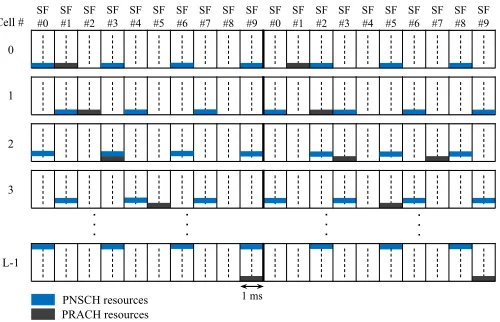
In this work we assume that inter-cell interference is negligi-ble. Inter-cell interference can be heavily mitigated, and there-fore, considered insignificant, if less-aggressive frequency-reuse (e.g., frequency-reuse of 3 or 7) is adopted [74]. Inter-cell interference manifests itself in two ways, namely, coherent and non-coherent interference, being the former caused by contaminating cells (i.e., cells that use the same set of pilots as the home cell, causing pilot-contamination) and the latter caused by non-contaminating cells (i.e., cells that do not use the same pilots as the home cell) [37]. In multi-cell scenarios, pilot-contamination, and consequently, coherent interference, can be disregarded once the PNSCH time-frequency resource intervals in each one of the neighbor cells can be configured to refrain them from overlapping with the intervals chosen for the target cell. This kind of configuration can be implemented in order to improve the overall system performance as pilot-contamination results in degradation of the channel estimate quality, which directly impacts on the spectral efficiency [37]. Figure 4 illustrates one possible configuration for the PNSCH intervals of neighbor cells so that pilot-contamination is mitigated.

We assume the utilization of OFDM block-based trans-missions. We denote the OFDM symbol interval by Ts, the

subcarrier spacing by ∆f, the useful symbol duration by Tu = 1/∆f, and the guard interval (duration of the cyclic

prefix) byTg=Ts−Tu. As in [39], we call the reciprocal of

the guard interval, when measured in subcarrier spacings, the ”frequency smoothness interval”,

Nsmooth=

1 Tg∆f

=Tu Tg

, (1)

whereNsmoothrepresents the number of subcarriers over which

the channel frequency response is considered smooth, i.e., approximately constant [37].

Fig. 3. Uplink Frame Structure with PNSCH.

IWT’2015

. . . . . . . . . . . .

Cell #

0

1

2

3 SF #0

SF #1

SF #2

SF #3

SF #4

SF #5

SF #6

SF #7

SF #8

SF #9

SF #0

SF #1

SF #2

SF #3

SF #4

SF #5

SF #6

SF #7

SF #8

SF #9

PNSCH resources PRACH resources

1 ms L-1

Fig. 4. Possible PNSCH resource configuration throughout different neighbor cells.

A total of τp OFDM symbols are used entirely for pilot

sequence transmission. The remaining symbols, τu, within

the same coherence block are used for data transmission. In general, the response is constant over Nsmooth consecutive

subcarriers and, therefore, the BS can estimate the channel for a total of Kmax=τpNsmooth terminals. We assume that a

coherence block consists of Nsmooth subcarriers and τp+τu

OFDM symbols, i.e., Nsmooth×(τp +τu) subcarriers, over

which the channel response is approximated as constant and flat-fading [41].

1) Pilot Transmission: as widely used in LTE systems [47], we adopt Zadoff-Chu sequences to design the mutually orthogonal pilot sequences allocated to the MTC devices. These sequences present unit-norm elements but also the addi-tional feature that each sequence is the cyclic shift of another sequence [66], [67]. However, any other set of sequences exhibiting the mutual orthogonality property could be used as pilot sequence,e.g., Walsh Hadamard sequences [68]. Within a cell, each terminal is assigned a τpNsmooth pilot sequence,

which is orthogonal to the pilot sequences that are assigned to other terminals in the cell. Collectively, theK≤τpNsmooth

terminals in the cell have the pilot book represented byΦ- a τpNsmooth×K unitary matrix such thatΦHΦ =IK. The pilot

sequence assigned to the k-th MTC device is represented by the column vectorφk.

2) Data transmission: we assume that the modulated sym-bols (carrying data of a MTC device) are randomly and independently drawn from a digital modulation alphabet (e.g., PSK, 16QAM, etc.) with normalized average energy. The modulated symbols are mapped intoτu OFDM symbols.

Each MTC device transmits its signal (i.e., allocated pi-lot sequence and data) by taking the Inverse Fast Fourier Transform (IFFT) of the mapped pilot sequence and data, and subsequently adding a CP.

(7)

7

IWT’2015

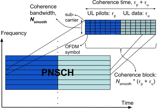
The time-frequency plane

UL pilots: _p UL data: _u Coherence time, _p + _u Coherence

bandwidth,

N_smooth

sub-carrier

. . .

. .

. _Time

PNSCH

The time-frequency plane is divided into coherence blocks in which each channel is time-invariant and frequency-flat

Frequency

OFDM symbol

Coherence block:

N_smooth * (_p + _u)

Fig. 5. Time-frequency plane.

blocks in which each channel is time-invariant and frequency-flat. The fraction of pilot symbols and UL data can be selected based on the network traffic characteristics, i.e., the PNSCH configuration can be modified to increase the number of served MTC devices or the data rate per MTC device by increasing the number of OFDM symbols used for pilot or data transmission accordingly.

As can be seen in Figure 2, filters are added to both transmission and reception chains. These filters are added to the processing chains so that out-of-band emissions (OOBE), which are intrinsic to the OFDM waveform due to the discon-tinuities at its edges, do not interfere with adjacent channels, i.e., Physical Random Access Channel (PRACH), Physical Uplink Shared Channel (PUSCH) and Physical Uplink Control Channel (PUCCH). Additionally, the filters help to mitigate inter-symbol interference (ISI) and inter-carrier interference (ICI) caused by asynchronous transmissions coming random access attempts happening at the PRACH [69]. Note that the received signal is passed through a matched filter, which maximizes the signal-to-noise ratio (SNR). The filter is applied to each time domain OFDM symbol (i.e., after IFFT and CP insertion) to mitigate the OOBE of the PNSCH transmissions. The filters should be carefully designed to (i) maintain the complex-domain orthogonality of OFDM symbols, (ii) exhibit flat passband over the subcarriers in the PNSCH, (iii) have sharp transition band in order to reduce the guard-bands, and (iv) present sufficient stop-band attenuation [70].

B. The Massive MIMO Channel

Let hm,k,n denote the complex propagation coefficient

between the m-th BS antenna and the k-th MTC device in the n-th subcarrier

hm,k,n=gm,k,n

p

dk, (2)

wheregm,k,nis a complex small-scale fading coefficient, and

dk is an amplitude coefficient that accounts for geometric

attenuation and shadowing, i.e. large-scale fading [39]. The large-scale fading coefficients are assumed constant with re-spect to both subcarrier number and with rere-spect to the index

…

BS

- terminals per cell.

-

BS co-located antennas.

ℎ

,

Signal from

k-

th user to the

m-

th BS antenna.

Problem definition

Fig. 6. Propagation model.

of the BS antenna since the geometric and shadow fading change slowly over space [39]. Therefore, between any given BS and a MTC device, there is only one large-scale fading coefficient. Additionally, these coefficients change only when a MTC device significantly change its position. It is normally assumed that in the radius of 10 wavelengths, the large-scale fading coefficients are approximately constant. On the other hand, small-scale fading coefficients significantly change as soon as the MTC device moves by a quarter of the wavelength. Therefore, the large-scale fading coefficients change about 40 times slower than the small-scale fading coefficients [71].

The random channel responses in one coherence block are statistically identical to the ones in any other coherence block, irrespective of whether they are separated in time and/or frequency. Hence, the channel fading is described by a stationary ergodic random process. Therefore, hereafter, our analysis is carried out by studying a single statistically representative coherence block. We assume that the channel realizations are independent between any pair of blocks, which is known as a block fading assumption. Consequently, for notational simplicity we suppress the dependency of hm,k,n

on the subcarrier index and write it ashm,k (see Figure 6).

The elementshm,k of theM ×K channel matrix

H= [h1 h2 . . . hK]

=



 

g1,1 · · · g1,K

..

. . .. ...

gM,1 · · · gM,K



 

| {z }

G

.



 

d1 . ._.

dK



 

| {z }

D

1/2

, (3)

correspond to the complex channel gains from the trans-mit antennas to the receive antennas, where hk ∼

CN(0M, bkIM), ∀k. The channel model in (3) is called

uncorrelated Rayleigh fading or independent and identically distributed (i.i.d.) Rayleigh fading, because the elements of

hk, i.e., hm,k, are uncorrelated (and also independent) and

have Rayleigh distributed magnitudes.

Under the assumption of large M and that the small-scale fading coefficients experienced by each MTC device are i.i.d. random variables with zero mean and unit variance, the column channel vector from different MTC devices becomes

(8)

8

asymptotically orthogonal as the number of receive antennas at the BS grows without bound [39]

HHH=D1/2GHG D1/2M≈→ ∞MD1/2IKD1/2=MD, (4)

where (·)H denotes transpose-conjugate (Hermitian) oper-ation. As can be noticed, the small-scale fading vanishes and only the large-scale fading remains, however, it can be mitigated with power control techniques [72], [73].

One of the key assumptions exploited by massive MIMO systems is that the channel vectors between the BS and the terminals should be nearly orthogonal. This condition, which is shown in (4), is known in the literature asfavorable propagation. With the assumption of favorable propagation, linear processing techniques can achieve optimal performance. For instance, on the uplink side, simple linear detectors can be used to cancel out noise and interference. On the downlink side, by adopting linear beamforming techniques, the BS can simultaneously beamform multiple data streams to multiple terminals without causing mutual interference [74], [75]. We refer the eager reader to [76] for a discussion on this condition, and to [49] for some experimental evidence supporting the assumption of i.i.d. small-scale fading coefficients in Massive MIMO.

C. Linear MMSE Channel Estimation

Here we consider the case where CSI, i.e.,His estimated from the received pilot sequences at the BS. As mentioned earlier, we do not consider the existence of pilot-contamination during the channel estimation phase once the PNSCH intervals in all cells (target and neighbor ones) can be configured to avoid transmission overlapping.

1) De-Spreading of the Received Pilot Signal: the pilot se-quences propagate through the uplink channel and are received by the BS as a M ×τpNsmooth signal,

Y=√ρHΦH+W, (5)

whereρis the uplink transmit power (UL Tx power) and the elements of the M ×τpNsmooth receiver noise matrix, W, are

i.i.d. CN(0,1). The BS performs a de-spreading operation of the received signal by correlating it with each one of the K pilot sequences. This is the equivalent of right-multiplying the received signal matrix by thek-th pilot sequence,φk, resulting

in

y_k= Y√φk ρ

=HΦH φk+ Wφk

√ ρ

=hk+w’,

(6)

wherew’= W_√Φk

ρ is an M×1noise vector, whose elements

are i.i.d. CN(0,1/ρ) because they are related to the original Gaussian noise matrix by a unitary multiplication scaled by 1/√ρ. The de-spread signal, y_k, is Gaussian distributed as follows

y_k∼ CN

0M,

dk+

1 ρ

IM

. (7)

Remark 1: Asρ→ ∞, the variance ofyk→dk.

Equation (6) is also known as the Least Squares (LS) estimator [77],

ˆ

hLS_k =y_k, (8) and its mean-square estimation error per antenna is denoted by

ηLS_k = 1 ME[k

˜

hLS_k k2_{] =} 1 ME[k

ˆ

hLS_k −hkk2] =

1 ρ. (9)

The LS channel estimation error is correlated with both the channel estimate and the de-spread received signal,

1 ME[(˜h

LS k )

H_h_ˆLS k ] =

1 ME[(˜h

LS k )

H_y k] =

1

ρ. (10)

As the LS channel estimate, ˆhLS_k , the estimation error h˜LS_k

is also Gaussian distributed as follows,

˜

hLS_k ∼ CN

0M,

1 ρIM

. (11)

Next, we present the MMSE estimator, which exhibits better performance than that of the LS estimator [65].

2) Channel Estimation: After de-spreading, the BS has a noisy version of the channel vector, which is defined by (6). Under the assumption of independent Rayleigh fading, the elements of the channel vector and the noise vector are statistically independent. By assumption, the large-scale fading coefficients are considered known at the BS, so the prior distribution of hm,k ∼ CN(0, dk), is also known. In

section IV we outline a possible approach for estimation of the large-scale fading coefficients at the BS. The linear MMSE estimator is the estimator achieving minimum MSE among all estimators of such form [41]. That is, it solves the following the optimization problem

ˆ

hMMSE_k = arg min

B∈BM×Mkhk−Bykk 2_,

(12)

wherey_k is defined in (6), B is a matrix that minimizes the mean square error (MSE). After solving (12), we find that the linear MMSE channel estimator is given by

ˆ

hMMSE_k = dk dk+1_ρ

y_k

= ρdk

ρdk+ 1 y_k.

(13)

Note that as ρ → ∞, the MMSE estimator becomes the LS estimator. The mean-square per antenna of the channel estimate is denoted byγk and given by

γk=

1 ME[k

ˆ

hMMSE_k k2_{] =} ρd 2

k

1 +ρdk

. (14)

The channel estimation error is denoted by

˜

hMMSEk = ˆh MMSE

k −hk, (15)

and the mean-square estimation error per antenna is

ηkMMSE=

1 ME[k

˜

hMMSEk k2] =

1 ME[k

ˆ

hMMSEk −hkk2]

= dk

1 +ρdk

=dk−γk.

(9)

9

As ρ → ∞, the mean-square error (MSE) per antenna, ηMMSE

k →0.

The channel estimation error is uncorrelated with both the channel estimate and the de-spread received signal,

1 ME[(˜h

MMSE

k )

H_h_ˆMMSE

k ] = 0. (17)

1 ME[(˜h

MMSE

k )

H_y

k] = 0. (18)

The estimation error h˜MMSE_k and the estimate hˆMMSE_k are jointly Gaussian distributed as follows,

ˆ

hMMSE_k ∼ CN(0M, γkIM). (19)

˜

hMMSE_k ∼ CN(0M,(dk−γk)IM). (20)

Therefore, the fact that they are uncorrelated implies that they are also statistically independent.

Remark 2: Asρ→ ∞, the variance ofhˆMMSE_k →dk.

One final remark about the MMSE estimation is that the MMSE estimator of a Gaussian random variable, hk, that

is observed in independent Gaussian noise, w’, is a linear estimator and thus equals the linear MMSE channel estimator, i.e., there exist no better non-linear Bayesian estimator in this special case [41].

D. Signal Detection

Here we consider the scenario where the K MTC devices simultaneously transmit signals to the BS. Let xk, where E[|xk|2] = 1, ∀k, be the signal transmitted from the

k-th device to k-the BS. Since K devices share the same time-frequency resource, the M ×1 received signal vector at the BS is the combination of all signals transmitted from all K devices [38], [74]:

y=√ρH x+w

=√ρ

K

X

k=1

hk xk+w,

(21)

wherey∈CM×1,√ρxis theK×1vector of symbols

simulta-neously transmitted by theKdevices (the average transmitted power of each device is ρ) and w ∈ CM×1 is a zero-mean

noise vector with complex Gaussian distribution and identity covariance matrix, i.e., CN(0M,IM). The noise variance is

made unitary in order to minimize notation, but without any loss of generality. With this convention,ρcan be interpreted as normalized uplinktransmitSNR or as introduced in subsection III-C, UL Tx power, and is therefore dimensionless [78]. There exist M PNSCH signal versions in (21) for each of the K MTC devices. Hence, the task of the BS consists in detecting K simultaneous MTC transmissions on the basis of estimates of the channel coefficients in (3). Detection techniques need to be employed in order to separate each one of the data streams transmitted by the various devices in a Massive MIMO system. When it comes to separation of data streams in conventional systems, the complex signal processing technique known as Maximum Likelihood (ML) detection provides the optimal

performance. With ML detection, the BS has to search all possible transmitted signal vectorsx, and choose the best one as follows:

ˆ

x= arg min

x∈XKky− √

ρHxk2_, ₍₂₂₎

where X is the finite alphabet of xk, k = 1,2, . . . , K. The

problem (22) is a least squares (LS) problem with a finite-alphabet constraint. The BS has to search over|X|K _vectors,

where |X| denotes the cardinality of the set X. Hence, ML has a complexity which is exponential in the number of MTC devices,K. Therefore, although being the optimal solution for detection, ML is a highly complex solution to be implemented in our case, where hundreds to thousands of MTC devices are envisioned. This is the reason why signal detection is a key problem in Massive MIMO systems. To circumvent this limitation, we discuss in the next section a couple of sub-optimal alternatives with reduced computational complexity [77]. However, when the number of BS antennas is large, it is shown in [39], [49] that linear processing is nearly-optimal. We justify our choices for the detectors adopted in this work in the simulation work presented later on in Section VI.

E. Linear Decoding

Linear decoders (also known as linear detectors) work by spatially decoupling the effects of the channel by a process known as MIMO equalization. This involves multiplying y

with a MIMO equalization matrix A ∈ CM×K to get

ˆ

x(y)∈CM×1[77]. LetAbe anM×Klinear detector matrix

that depends on the estimated channel Hˆ. By using a linear detector, the received signal can be separated into different data streams using Aas follows

r=AHy, (23)

where the vectorrcollects the data streams received at the BS, i.e.the symbols of allKsingle-antenna MTC devices, andA

is a receive matrix that depends on the specific linear detector used at the BS. After linear detection, as seen in Figure 2, each data stream undergoes FFT processing and subcarrier extraction in order to retrieve data symbols.

Inspection of (3) reveals that D is a diagonal matrix, so we can use MRC in the uplink to separate the signals from different MTC devices into different streams with asymptotic no inter-user interference [39]. Thereby each MTC device’s transmission can be seen as signals of a single device passing through a single input single output channel. In the limit, this implies that MRC is optimal when the number of receive antennas is much larger than the number of transmit antennas, i.e. M K, M → ∞ – as can be seen from (4). In MRC the linear detection matrixAis chosen using

AMRC= ˆH (24)

where the dominant computation is due to matrix transposition. With MRC, the BS aims to maximize the received signal-to-noise ratio (SNR) of each MTC device,i.e., stream, ignoring the effect of multiuser interference and therefore, one of its drawbacks is that it performs poorly in interference-limited

(10)

10

scenarios [37]. The associated complexity is of onlyO(M K) multiplications.

In contrast to the MRC decoder, ZF decoders take the inter user interference into account, but neglect the effect of noise, i.e., it choosesAwith the objective of completely eliminating interference, regardless of noise enhancement. With ZF, the multiuser interference is completely nulled out by projecting each stream onto the orthogonal complement of the inter user interference [37]. Specifically, the ZF detector chooses

Aconstrained toAH=I

AZF= ˆH( ˆHHHˆ)−1. (25)

The advantages of ZF are that the signal processing is simple and it works well in interference-limited scenarios. The drawback is that since ZF neglects the effect of noise, it works poorly under noise-limited scenarios. Furthermore, if the channel is not well conditioned then the pseudo-inverse amplifies the noise significantly, and therefore, the performance is very poor. Compared with MRC, ZF has a higher implementation complexity due to the computation of the pseudo-inverse of the channel gain matrix [78]. ZF exhibits a complexity ofO(M K+2M K2_+K3₎_{[49]. A better strategy} is to chooseAso as to balance the signal energy lost with the increased interference. From this point of view, it is better to accept some residual interference provided that this allows the detector to capture more of the desired signal’s energy [77].

One last linear detector that, together with MRC and ZF, poses complexity costs that do not depend on the modulation order is the MMSE. As the name suggests, the MMSE detector chooses theAthat minimizese=E[kAH_y₋_x_k2_|_Hˆ_]_without any additional constraints

AMMSE= ˆH

ˆ

HHHˆ +1 ρcov

w−√ρH˜x

−1

= ˆH

"

ˆ

HHHˆ +1

ρ 1 +ρ

K

X

l=1

E

h

˜

hl˜h H l

i !

IK

#−1

, (26)

where cov(a) denotes the covariance matrix of a random variablea andH˜ is the estimation error, H= ˆH−H˜.

In contrast to ZF, which minimizes interference but fails to treat noise, and to MRC, which minimizes noise but fails to treat interference, MMSE achieves an optimal balance between interference suppression and noise enhancement (it maximizes the received SINR [78]) at the same cost (i.e., complexity) of ZF [49], [79].

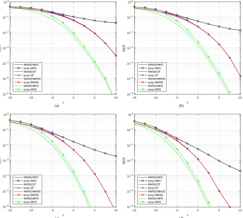
The shortcomings listed in Table I of [48] under iterative filtering, random step search, and tree-based methods suggest that these detection classes perform well but are still too complex to be practical. This indicates that more work is needed on this matter, perhaps towards turbo codes or Low-density Parity-check (LDPC) codes in iterative detection and decoding settings [80]. On the other hand, linear filtering meth-ods that are non-iterative, such as MRC, ZF, and MMSE, seem more feasible candidates for Massive MIMO systems. For 1KM, it is known that linear detection performs fairly well, and asymptotically achieves capacity when M → ∞. [39]. We therefore consider only such linear methods in the simulation work section.

F. Achievable Rates

In this subsection we derive lower bounds on the achievable rate for each one of the studied linear detectors when MMSE channel estimation is considered. Considering that during one PNSCH transmission interval at the target cell there are no other PNSCH transmissions being originated at other cells or that a less-aggressive frequency-reuse factor (e.g., reuse factor of 3 or 7 for instance) is employed, we can analyze and derive the achievable rates as if the target cell was a single-cell system, emphasizing the fact that inter-single-cell interference is inexistent or negligible and therefore, do not need to be accounted for. The rationale behind the single-cell Multi User (MU)-MIMO analysis is that its results are readily compre-hended, they bound the performance of multicell systems and that the single-cell performance can be actually achieved if less-aggressive frequency-reuse is adopted. For the following derivations we use standard capacity bounding techniques from the massive MIMO literature [37], [74], [81].

The received signal vector at the BS can be rewritten as

r=AH√ρHˆx−√ρH˜x+w, (27)

where H˜ = ˆH−H. Due to the properties of the MMSE estimation, H˜ is independent of Hˆ, see (17). Therefore, the received signal associated with the k-th MTC device is given by

rk =

√

ρaH_k Hˆx−√ρaH_k H˜x+aH_k w

=√ρaH_k ˆhkxk

| {z }

desired signal

+√ρ

K

X

l=1,l6=k aH_kˆhlxl

| {z }

intra-cell interference

−√ρ

K

X

l=1

aH_kh˜lxl+aHk w

| {z }

effective noise

,

(28)

where ak, hˆl and h˜l are the l-th columns of A, Hˆ, and

˜

H, respectively. As H˜ and Hˆ are independent, A and H˜

are also independent. As shown in (28), the BS treats the channel estimate as the true channel, and the last three terms in the equation are considered as intra-cell interference and effective noise respectively. Therefore, an achievable rate of uplink transmission for thek-th MTC device is defined by

Rk=E{log2(1 +SINRk)}, (29)

SINRk =

ρ|aH_k ˆhk|2

ρPK

l=1,l6=k|aHkhˆl|2+ρkakk2P K

l=1ηMMSEl +kakk2

,

(30)

(11)

11

1) MRC detector: with MMSE channel estimation, Rayleigh fading, and MRC processing, the achievable rate for the k-th MTC device is lower bounded by

˜

RMRC_k = log₂ 1 + ρ(M−1)γk 1 +ρPK

l=1dl−ργk

!

. (31)

2) ZF detector: with MMSE channel estimation, Rayleigh fading, ZF processing, and forM ≥K+ 1the achievable rate for the k-th MTC device is lower bounded by

˜

RZF_k = log₂ 1 + ργk(M−K) 1 +ρPK

l=1η

MMSE l

!

. (32)

3) MMSE detector: with MMSE channel estimation, Rayleigh fading, MMSE processing, the achievable rate for the k-th MTC device is approximately lower bounded by

˜

RMMSEk = log2(1 + (αk−1)θk), (33)

where

αk=

(M−K+ 1 + (K−1)µ)2

M −K+ 1 + (K−1)κ , (34)

θk=

M−K+ 1 + (K−1)κ

M−K+ 1 + (K−1)µwγk, (35)

where w =h1_ρ+PK

l=1ηMMSEl

i−1

, µ and κare obtained by solving the following two equations:

µ= 1

K−1

K

X

l=1,l6=k

1

M wγl 1−K_M−1 +K_M−1µ+ 1

(36)

κ



1 +

K

X

l=1,l6=k

wγl

M wγl 1−KM−1+ K−1

M µ

+ 12 



=

K

X

l=1,l6=k

wγlµ+ 1

M wγl 1−KM−1+ K−1

M µ

+ 12

(37)

IV. ESTIMATION OFLARGE-SCALEFADINGCOEFFICIENTS

In this section we describe how the large-scale fading coeffi-cients,dk,∀k, can be estimated based on the de-spread signal, yk. We employ the Maximum Likelihood (ML) method to

estimate the the large-scale fading coefficients [82]. Applying the ML method to f(y_k;dk) with distribution defined in (7),

we find the following estimator for dk given the observation y_k

ˆ dk =

ky_kk2

M −

1

ρ. (38)

This estimator exhibits a central Chi-square distribution with 2M degrees of freedom. It has E[ ˆdk] = dk, which shows

that the ML estimator is unbiased, and var( ˆdk) =

(dk+1ρ) 2

M .

The mean-square error of the proposed large-scale fading coefficient estimator is defined as

E[(dk−dˆk)2] =

dk+1_ρ

2

M . (39)

Note that the mean-square error of the proposed estimator is also equal to its variance.

Remark 3:AsM → ∞,E[(dk−dˆk)2] =var( ˆdk)→0.

Remark 3 shows that as M increases, the estimator defined in (38) becomes a deterministic value and that it tends, in the limit, to the actual dk value once the mean-square error

vanishes.

In order to assess the efficiency of the estimator we derive the Cram´er-Rao bound as [82]

var( ˆdk)≥

(dk+1_ρ)2

M . (40)

Therefore, as can be noticed, the ML estimator derived for dkis the minimum variance unbiased estimator (MVUE),i.e.,

it is an unbiased estimator that has the lowest variance among all other possible unbiased estimators [82].

Additionally, we show that the proposed estimator ap-proachesdk as the number of antennasM increases.

lim

M→∞ ˆ

dk = lim M→∞

ky_kk2

M −

1 ρ

a.s.

=dk. (41)

The proof of (41) is provided in Appendix A. This is an example of the strong law of large numbers and can be interpreted as the variations of kykk2

M becoming increasingly

concentrated around its mean value E

h_k_y

kk2

M

i

= dk+ 1_ρ as

more antennas are added.

V. PROPOSEDCHANNELESTIMATOR

In this section we propose a simple and practical channel estimator based on the estimator for the large-scale fading coefficients defined in Section IV. Our proposed approach estimates the large-scale fading coefficients,dk, and replaces

it into the MMSE channel estimator defined in (13), resulting in the following channel estimator

ˆ

hprop_k =

1−M

ρ 1 ky_kk2

y_k. (42)

Remark 4: The proposed estimator asymptotically ap-proaches the ideal MMSE channel estimator in (13) asM → ∞,

lim

M→∞

1−1 ρ

M ky_kk2

y_k=

_ρd

k

ρdk+ 1

y_k. (43)

This can be easily proved by applying Lemma 4 to (42). The proposed estimator has E

h

ˆ

hprop_k i =0M and covariance

matrix given by

Cov[ˆhprop_k ] =_E[ˆhprop_k (ˆhprop_k )H] =(ρdk+ 1)(ρdk−1)(M−1) +M

ρ(ρdk+ 1)(M−1)

IM

= ρd

2

k

(ρdk+ 1)

+ 1

ρ(ρdk+ 1)(M −1) IM

=γk+k,

(44)

(12)

12

wherek = _ρ₍_ρd_k₊₁₎₍1 _M₋₁₎, which is the error introduced by

the estimation of dk.

Remark 5: AsρandM → ∞, the variance ofhˆprop_k →dk.

As can be seen by analyzing equation (44), as M → ∞, Cov[ˆhprop_k ] → ρd2k

1+ρdkIM, which is the covariance matrix of the MMSE estimator. The mean-square estimation error per antenna of the proposed channel estimator is defined as

η_kprop= 1 ME[k˜h

prop k k

2_{] =} 1 ME[khˆ

prop

k −hkk2]

= 1

ρ

_M

M−1 1 1 +ρdk

−1 + 2θk

,

(45)

where θk =

R1

0

R1 −1

κ2_k(1−t)+κkw √

t(1−t)

κ2

k(1−t)+2κkw √

t(1−t)+tfW(w)fT(t)dwdt

andκk,

√

ρdk andfW(w)andfT(t)are defined by

fT(t) =

Γ(2M)

(Γ(M))2[t(1−t)]

M−1

, 0< t <1, (46)

fW(w) =

M πB

₁

2, M

1−w2M− 1

2_, _|_w_|_<_1. ₍₄₇₎

The proof of the mean-square estimation error per antenna is given in Appendix B. The analytical mean-square estimation error expression (45) is useful for system design and perfor-mance evaluation purposes [83].

Remark 6:The mean-square error betweenˆhprop_k andhˆMMSE_k

is defined as

1 ME[k

ˆ

hpropk −ˆh MMSE k k2] =

1

ρ(ρdk+ 1)(M−1)

=k. (48)

The proof of (48) is given in Appendix C. From (48) we observe that the mean-square error decreases when M, ρ anddk increase, which consequently shows that the proposed

channel estimator asymptotically approaches the performance of MMSE channel estimator.

-20 -10 0 10 20 30

[dB]

10-3 10-2 10-1 100 101 102

MSE

LS (analytical) LS (simulated) MMSE (analytical) MMSE (simulated) Prop. (analytical) Prop. (approximated) Prop. (simulated)

Fig. 7. Channel estimation MSE versus uplink pilot power,ρ.

20 40 60 80 100 120 140 160 180 200

M

0.09 0.092 0.094 0.096 0.098 0.1

MSE

Fig. 8. MSE performance versus number antennas,M.

Next, we also present a simpler and more tractable expres-sion for the mean-square estimation error per antenna, which is defined as

1 ME[kh˜

prop k k

2_{] =} 1 ME[kˆh

prop

k −hkk2]≈η

prop(approx.)

k =

=1

ρ

ρdk

1 +ρdk

+ 1

(M −1)(1 +ρdk)

=dk−γk+k.

(49)

Remark 7:AsM orρ→ ∞,η_kprop(approx.)=dk/(1 +ρdk) =

dk−γk.

Remark 7 clearly shows that the approximated mean-square estimation error per antenna of the proposed estimator tends to that of the MMSE estimator whenM → ∞. The proof for the approximated mean-square estimation error per antenna of the proposed channel estimator is given in Appendix D.

The channel estimation error is correlated with the channel estimate and uncorrelated with the de-spread received signal,

1 ME[(˜h

prop k )Hˆh

prop

k ] =k. (50)

1 ME[(˜h

prop k )

H_y

k] = 0. (51)

Remark 8:AsM or ρ→ ∞, then _M1_E[(˜hprop_k )H_h_ˆprop k ] = 0.

The estimation error,h˜propk , have the following mean vector

and covariance matrix,

E[˜h prop

k ] =0M, (52)

(13)

13

A. Complexity Analysis

The computational complexity is a important factor indicat-ing the efficiency of a channel estimator. In this section we assess the computational complexity of the studied channel estimators. Table II summarizes the complexities involved in the calculation of the estimators in terms of number of floating-point operations (flops) and the Big-O notation. The Big-O notation, also called Landau’s symbol, which is a well-known symbolism widely used in complexity theory to describe the asymptotic behavior of algorithms [84]. It basically indicates how fast an algorithm grows or declines. In the table P is the length of the pilot sequence (i.e., τpNsmooth) and D is a

K×K identity matrix with the diagonal elements equal to

ρdk

ρdk+1 ∀kand

1−M

ρ

1 ky_kk2

∀kfor the MMSE and proposed channel estimators respectively. It is important to notice that in this work and in the great majority of works in the literature [65], [85]–[87] the large scale fading coefficients, {dk}, are

assumed perfectly known for the MMSE channel estimation. The LS estimator is the most computational cost efficient among all of them, presenting a complexity of O(M P K), however, as will be shown later, this is the least efficient estimator in terms of MSE. The MMSE estimator is the most efficient in terms of MSE, exhibiting a complexity of O(M K(P + K)), however, as mentioned earlier, the complexity involved in the calculation of large-scale fading coefficients (i.e., the elements ofD) is not taken into account. On the other hand, the proposed estimator, presents MSE efficiency that asymptotically approaches that of the MMSE estimator and has a complexity ofO(M K(P+K+1)), where the calculation (i.e., estimation) of the large-scale fading coefficients is already considered in the presented complexity.

VI. SIMULATIONRESULTS

In this section, we compare the performance of the pro-posed channel estimator with that of LS and MMSE channel estimators. Additionally, we assess the performance of MRC, ZF, and MMSE linear decoders when the MMSE and the proposed channel estimators are employed. The performance of each linear decoder is quantified in terms of its Bit Error Rate (BER) over a range of UL Tx power (i.e.,ρ) values.

We consider two different types of simulation setups for the large-scale fading coefficient, dk, one with fixed values and

other with random values. For the fixed case, we set dk= 1.

For the random case, the MTC devices in the cell (see Figure 6) are uniformly distributed within a ring with radii r0 = 100 m and r1 = 1000 m respectively. The large-scale fading coefficients{dk}are independently generated bydk=

ψ/rk

r0

v

, where v = 3.8, 10 log₁₀(ψ) ∼ N(0, σ2

shadow,dB)

with σshadow,dB = 8, and rk is the distance of the k-th MTC

device to the BS. Both, the path loss exponent, v, and the standard deviation of the log-normal shadowing, σshadow,dB,

are common values for outdoor shadowed urban cellular radio environments [88], [89]. For all simulations we assume K= 10MTC devices.

Figure 7 shows the MSE versus UL Tx power results (ρ) for the case whendk= 1andM = 70. As can be noticed, the

analytical, approximated and simulated MSE curves match for all the studied channel estimators. As expected, the MSE of all estimators decreases as ρ increases. At low ρ values (values lower than -10 dB), the MSE of the proposed estimator is higher than that of the MMSE estimator, however, it is still smaller than that of the LS estimator. On the other hand, with the increase of ρ (for values higher than -10 dB), the gap between the MMSE and proposed estimators decreases.

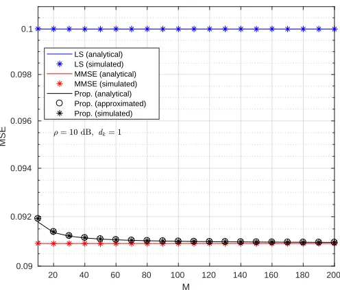
The MSE versus the number of BS antennas,M, is com-pared in Figure 8 for the case when dk = 1 andρ= 10 dB.

The MSE of the proposed estimator decreases asM increases, approaching the MSE of the MMSE estimator, while the MSE of the LS and MMSE channel estimators stay constant. The result showed in the figure is in line with Remark 4. Additionally, it is also worth mentioning that the approximated MSE expression for the proposed channel estimator matches the values of the closed-form expression.

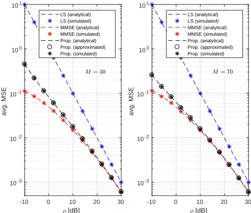
In Figure 9, we assess the variation of the MSE under random large-scale fading {dk} for M = 30 and M = 70

respectively. The results are obtained by averaging the MSE values over10×103 _{realizations of}_{_d

k}. As can be noticed,

the simulated MSE values match the values of the analytical and approximated MSE expressions. It can be also noticed that the MSE of the proposed channel estimator approaches that of the MMSE channel estimator asM increases. The pro-posed channel estimator outperforms the LS channel estimator significantly at low UL Tx power values.

Figures 10 and 11 present the averaged variance and error under random large-scale fading coefficient, {dk},

respec-tively. The results are obtained by averaging the variance and error values over 10×106 _{different realizations of}_{_d

k}. As

can be seen, the variance and consequently the error of the LS and MMSE channel estimators do not depend onM (both of them depend only on ρ), however, the variance of the proposed channel estimator depends on both M and ρ. As M increases, the variance curve for the the proposed channel

-10 0 10 20 30

[dB] 10-3

10-2

10-1 100

101

avg. MSE

-10 0 10 20 30

[dB] 10-3

10-2

10-1 100

101

avg. MSE

Fig. 9. Average channel estimation MSE under randomdk versus uplink

pilot power,ρ.

(14)

14

TABLE II

COMPLEXITIES INVOLVED IN THE STUDIED LINEAR CHANNEL ESTIMATORS.

Estimator Operation Flops O(.)

LS YΦ M K(2P−1)or2M KP ifP is large M KP

MMSE/Prop.

YΦD M K(2P−1) +M K(2K−1)or2M K(P+K)ifP andKare large M K(P+K)

Calculation of the elements inD MMSE: Elements are considered perfectly known

-Prop.: calculation ofkykk2∀k:K(2M−1)flops or2KMifMis large M K

-10 -5 0 5 10 15 20 25 30 35 40

[dB]

10-2 100 102

Variance

LS estimator

M = 10 M = 100 M = 500 M = 1000 Avg. d_k = 0.2162

-10 -5 0 5 10 15 20 25 30 35 40

[dB]

10-4 10-2 100

Variance

MMSE estimator

M = 10 M = 100 M = 500 M = 1000 Avg. d_k = 0.2162

-10 -5 0 5 10 15 20 25 30 35 40

[dB]

10-2 100 102

Variance

Proposed estimator

M = 10 M = 100 M = 500 M = 1000 Avg. d_k = 0.2162

Fig. 10. Comparison of the averaged variances of the channel estimators.

estimator approaches that of the MMSE channel estimator. It is also worth mentioning that the variance of both MMSE and proposed channel estimators converges faster to the average dk than the variance of the LS estimator as can be seen in

Figure 11. These results are in line with Remarks 1, 2 and 5,

-10 -5 0 5 10 15 20 25 30 35 40

[dB]

10-4 10-2 100 102

Error

LS estimator

M = 10 M = 100 M = 500 M = 1000

-10 -5 0 5 10 15 20 25 30 35 40

[dB]

10-4 10-2 100

Error

MMSE estimator

M = 10 M = 100 M = 500 M = 1000

-10 -5 0 5 10 15 20 25 30 35 40

[dB]

10-4 10-2 100

Error

Prop. estimator

M = 10 M = 100 M = 500 M = 1000

Fig. 11. Average of the absolute error between the large-scale fading, dk,

and the variance of the studied estimators.

0 20 40 60 80 100

[dB] 10-20

10-10 100

Distance between estimators

Simulated

M = 10 M = 30 M = 100 M = 200 M = 500

0 20 40 60 80 100

[dB] 10-20

10-10 100

Distance between estimators

Analytical

M = 10 M = 30 M = 100 M = 200 M = 500

Fig. 12. Averaged distance between proposed and MMSE channel estimators.

showing that the variance of all the studied channel estimators tend to the averagedk.

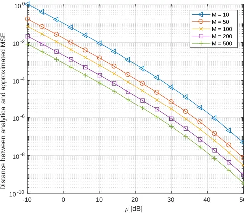
The averaged distance between the proposed and MMSE channel estimators for different number of antennas, M, and

-10 0 10 20 30 40 50

[dB]

10-10 10-8 10-6 10-4 10-2 100

Distance between analytical and approximated MSE

M = 10 M = 50 M = 100 M = 200 M = 500

On the Application of Massive MIMO Systems to Machine Type Communications