Data Accessibility for Resource Selection in Large-Scale Distributed Systems

Data Accessibility for Resource Selection in

Large-Scale Distributed Systems

Bachina Anusha#1 P.Venkata SubbaReddy#2 T.V. Sai Krishna#3

M.Tech Student, Associate Professor in CSE Associate Professor in CSE

QIS College of Engg &Tech., QIS College of Engg &Tech QIS College of Engg &Tech

Ongole,A.P, Ongole,A.P Ongole,A.P

Abstract—Large-scale distributed systems provide an attractive scalable infrastructure for network applications. However, the loosely coupled nature of this environment can make data access unpredictable, and in the limit, unavailable. We introduce the notion of accessibility to capture both availability and performance. An increasing number of data-intensive applications require not only considerations of node computation power but also accessibility for adequate job allocations. For instance, selecting a node with intolerably slow connections can offset any benefit to running on a fast node. In this paper, we present accessibility-aware resource selection techniques by which it is possible to choose nodes that will have efficient data access to remote data sources. We show that the local data access observations collected from a node’s neighbors are sufficient to characterize accessibility for that node. By conducting trace-based, synthetic experiments on Planet Lab, we show that the resource selection heuristics guided by this principle significantly outperform conventional techniques such as latency-based or random allocations. The suggested techniques are also shown to be stable even under churn despite the loss of prior observations.

Keywords—Data Accessibility, resource selection, passive network performance estimation, data-intensive computing, large-scale distributed systems.

1 I

L

scalable infrastructure for network applications. This virtue has led to the deployment of several distributed systems in large-scale, loosely coupled environments such as peer-to-peer computing [1], distributed storage systems [2], [3], [4], and Grids [5], [6], [7]. In particular, the ability of large-scale systems to harvest idle cycles of geographically distributed nodes has led to a growing interest in cycle-sharing systems [8] and @home projects [9], [10]. However, a major challenge in such systems is the network unpredictability and limited bandwidth available for data dissemination. For instance, the BOINC project [11] reports an average throughput of only about 289 Kbps, and a significant proportion of BOINC hosts shows an average throughput of less than 100 Kbps [1]. In such an environment, even a few megabytes of data transfer between poorly connected nodes can have a large impact on the overall application performance. This has severely restricted the amount of data used in such computation platforms, with most computations taking place on small data objects.

Emerging scientific applications, however, are data-intensive and require access to a significant amount of dispersed data. Such data-intensive applications encompass a variety of domains such as high-energy physics [12], climate prediction [13], astronomy [14], and bioinformatics [15]. For example, in high-energy physics applications such as the Large Hadron Collider (LHC), thousands of physicists worldwide will require access to shared, im-mutable data at the scale of pet bytes [16]. Similarly, in the area of bioinformatics, a set of gene sequences could be transferred from a remote database to enable comparison with

Input sequences [17]. In these examples, performance depends critically on efficient data delivery to the computational nodes. Moreover, the efficiency of data delivery for such applications would critically depend on the location of data and the point of access. Hence, in order to accommodate data-intensive applications in loosely coupled distributed systems, it is essential to consider not only the computational capability, but also the data accessibility of computational nodes to the required data objects. The focus of this paper is on developing resource selection techniques suitable for such data-intensive applications in large-scale computational platforms.

Data availability has been widely studied over the past few years as a key metric for storage systems [2], [3], [4]. However, availability is primarily used as a server-side metric that ignores client-side accessibility of data. While availability implies that at least one instance of the data is present in the system at any given time, it does not imply that the data are always accessible from any part of the system. For example, while a file may be available with 5 nines (i.e., 99.999 percent availability) in the system, real access from different parts of the system can fail due to reasons such as misconfiguration, intolerably slow connections, and other networking problems. Similarly, the availability metric is silent about the efficiency of access from different parts of the network. For example, even if a file is available to two different clients, one may have a much worse connection to the file server, resulting in much greater download time compared to the other. Therefore, in the context of data-intensive applications, it is important to consider the metric of data accessibility: how efficiently a node can access a given data object in the system.

The challenge we address is the characterization of accessibility from individual client nodes in large distributed systems. This is complicated by the dynamics of wide-area networks, which rule out static a priori measurement, and the cost of on-demand information gathering, which rules out active probing. Additionally, relying on global knowledge obstructs scalability, so any practical approach must rely on local information. To achieve accessibility-aware resource selection, we exploit local historical data access observations. This has several benefits. First, it is fully scalable as it does not require global knowledge of the system. Second, it is inexpensive as we employ observations of the node itself and its directly connected neighbors (i.e., one-hop away). Third, past observations are helpful to characterize the access behavior of the node. For example, a node with a thin access link is likely to show slow access most of the time. Last, by exploiting relevant access information from the neighbors, it is possible to obviate the need for explicit probing (e.g., to determine network performance to the server), thus mini-mizing system and network overhead.

Our key research contributions are as follows:

. We present accessibility estimation heuristics which employ local data access observations, and demon-strate that the estimated data download times are fairly close to real measurements, with 90 percent of the estimates lying within 0.5 relative error in live experimentation on PlanetLab.

. We infer the latency to the server based on the prior neighbor measurement without explicitly probing the server. For this, we extend existing estimation heuristics [18], [19], [20] to more accurately work with a limited number of neighbors. Our enhancement gives accurate results even with only a few neighbors.

. We present accessibility-aware resource selection techniques based on our estimation functions and compare to the optimal and conventional techniques such as latency-based and random selection. Our results indicate that our approach not only outper-forms the conventional techniques, but does so over a wide range of operating conditions.

. We investigate the impact of churn prevalent in loosely coupled distributed systems. In fact, churn is critical to our resource selection techniques because we assume that nodes lose all past observations when they join the system again. Despite this stringent memory-loss property, the results show that our techniques perform well even under a certain degree of churn.

2 A

-B

R

S

In this section, we present our system model followed by an overview of the accessibility-based resource selection algorithm that uses data accessibility to select appropriate compute nodes in the system.

2.1 System Model

Our system model consists of a network of compute nodes that provide computational resources for executing applica-tion jobs and data nodes that store data objects required for computation.

In our context, data objects can be files, database records, or any other data representations. We assume that both compute and data nodes are connected in an overlay structure. We do not assume any specific type of organization for the overlay. It can be constructed by using typical overlay network architectures such as unstructured [21], [22] and structured [23], [24], [25], [26], or any other techniques. However, we assume that the system provides built-in functions for object store and retrieval so that objects can be disseminated and accessed by any node across the system. Each node in the network can be a compute node, data node, or both.

Since scalability is one of our key requirements, we do not assume any centralized entities holding system-wide information. For this reason, any node in the system can submit a job in our system model. A job is defined as a unit of work which performs computation on an object. To allocate a job, a submission node, called an initiator selects a compute node from a set of candidates. We assume the use of a resource discovery algorithm [7], [8], [27], to determine the set of candidate nodes, though it may not consider data locality in its choice. Once the initiator selects a node, the job is transferred to the selected node, called a worker. The worker then downloads the data object required for the job from the network and performs the computation. When the job execution is finished, the worker returns the result to the initiator.

Formally, job J_i is defined as a computation unit which requires object o_i to complete the task. We assume that objects, e.g., o_i, have already been staged in the network and perhaps replicated to a set of nodes R_i ¼ fr1_i; r2_i; :::g based upon projected demand. The job J_i is submitted by the initiator. From the given candidates C¼ fc₁; c₂; :::g, the initiator selects one (i.e., worker2C) to allocate the job.

2.2 Resource Selection

Fig. 1 illustrates the resource selection process in our system model once the initiator has a set of candidate nodes to choose from. To select one of the given candidates, the initiator first queries the candidates for relevant information that can be used for job allocation, since there is no entity with global information (Fig. 1a). The candidates offer the relevant information (Fig. 1b), based on which, the initiator allocates the job to the selected worker (Fig. 1c). To incorporate the impact of data access on the performance of job execution, our goal is to select the best candidate node in terms of accessibility to a data node (server) holding object o_i.

Due to the decentralized nature of our system, we would like to make this selection without assuming any global knowledge. To achieve this goal, we use an accessibility-based ranking function to order the different candidate nodes. Sinceour goal is to maximize the efficiency of data access from the selected worker node, we use the expected data download time as the metric to quantify accessibility. Thus, given a set of candidates C for job J_i that requires access to object o_i, each candidate node c_m returns its accessibility accessibility_cm ðJiÞ in terms of the

estimated download time for the object o_i, and

Fig. 1. Accessibility-based resource selection. (a) Initiator asks accessibility estimation to candidates. (b) Candidate offers estimated accessibility to initiator. (c) Initiator selects the best candidate based on the reported accessibility.

the initiator then selects the node with the smallest accessibility value. Note that since we are assuming lack of any global knowledge, these estimates are based on the local information available to the individual candidate nodes. Therefore, sometimes the candidate cannot provide any meaningful estimate of its accessibility to the required data object. In this case, the candidate simply returns a value of 1, indicating the lack of any information. The initiator would filter out such a candidate. If all candidates return 1, one of the candidates is randomly selected. Formally, the selection heuristic H_s is defined as follows:

H_s : C ! c_m such that

accessibility

cmð

J

iÞ ¼ n

min

1;::;C ðaccessibility_cn ðJiÞÞ:

¼ j j

Having described the accessibility-based resource selection process, the question is how the candidate nodes can estimate their accessibility using local information (e.g., their own observations to the object if known or their neighbors), and what factors they can use for this estimation. We explore this question in the next section.

3 A

E

3.1 Accessibility Parameters

To answer the above question, we first investigate what parameters would impact accessibility in terms of data download time. Intuitively, a node’s accessibility to a data

object will depend on two main factors: the location of the data object with respect to the node and the node’s network characteristics such as its connectivity, bandwidth, and other networking capabilities. We have explored a variety of parameters to characterize these factors, and found some interesting correlations. For this characterization, we con-ducted experiments on Planet Lab [28] with 133 hosts over three weeks. In these experiments, eighteen 2 MB data objects were randomly distributed over the nodes, and over 14,000 download operations were carried out to form a detailed trace of data download times. To measure internodes latencies, an ICMP ping test was repeated nine times over the three-week period, and the minimal latency was selected to represent the latency for each pair. We next give a brief description of the main results of this study.

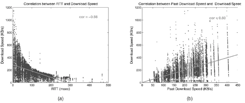
The first result is the correlation of latency and download speed (defined as the ratio of downloaded data size and download time) between node pairs. Fig. 2a plots the relationship between RTT and download speed. We find a negative correlation ðr¼

₃0:56Þ between them, indicating that smaller latency between client and server would lead to better performance in downloading. Thus, latency can be a useful factor when estimating accessibility between node pairs.

In addition, we discovered a correlation between the download speed of a node for a given object and the past average download speed of the node, as shown in Fig. 2b (r¼ 0:6). The intuition behind this correlation is that past download behavior may be helpful to characterize the node in terms of its network characteristics such as its con-nectivity and bandwidth. For example, if a node is

Fig. 2. Correlations of access parameters. (a) Correlation of RTT and download speed. (b) Correlation of download speed and past average

connected to the network with a bad access link, it is almost certain that the node will yield low performance in data access to any data source. This result suggests that past download behavior of a node can be a useful component for accessibility estimation.

Based on the statistical correlations we discovered, we next present estimation techniques to predict data access capabilities of a node for a data object. Note that we do not assume global knowledge of these parameters (e.g., pair-wise latencies between different nodes), but use hints based on local information at candidate nodes to get accessibility estimates. It is worth mentioning that it is not necessary to estimate the exact download time; rather our intention is to rank nodes based on accessibility so that we can choose a good node for job allocation. Nonetheless, if the estimation has little relevance to the real performance, then the ranking may deviate far from the desired choices. Hence, we require that the estimation techniques demonstrate sufficiently accurate results which can be bounded within a tolerable error range.

3.2 Self-Estimation

As described in Section 3.1, latency to the server1 and download speed of a node are useful to assess its accessibility to a data object. We first provide an estimation technique that uses historical observations made by a node during its previous downloads to estimate these parameters. Note that these past downloads can be to any objects and need not be for the object in question. We refer to this technique as self-estimation.

To employ past observations in the estimation process, we assume that the node records access information it has observed. Suppose Hi_h is the ith download entry at host h. This entry includes following information: object name, object size, download elapsed time, server, distance to server, and time stamp. As a convention, we use dotð:Þ notation to refer to an item of the entry, for example, Hi_h:size represents the object size in the ith observation at host h, and jH_hj denotes the number of observations at host h.

We first estimate a distance factor between the node and the server, based on their internode latency. For this, we consider several related latency models for the distance metric: RTT and square root of RTT. These are often used in TCP studies to cope with congestion efficiently to improve system throughput. Studies of window-based [32] and rate-based [33] congestion control revealed that RTT and square root of RTT are inversely proportional to system through-put, respectively. We consider both latency models for the distance metric and compare them to see which is preferable later in this section. The mean distance of node h to the servers is then computed by

1 X

Distance

h

_jH

_j

:distance:

We then characterize the network characteristics of the node by estimating its mean download speed based on

prior observations. The mean download speed of node h is defined as

jHhj i

DownSpeed_h ¼ 1

₃

X

jH j ¼H

Using the above factors, we estimate the expected download time for a host h to download object o as

SelfEstim_hðoÞ ¼ ₃₃_DownSpeedsizeðoÞ ; ð1Þ

h

where

₃

¼

distance

hð

server

o

_:

Distance_h

Here, sizeðoÞ means the size of object o, serverðoÞ means the server for object o, and distance_aðbÞ means the distance between nodes a and b.

Intuitively, The parameter ₃ gives a ratio of the distance to the server for object o to the mean distance it has observed. Smaller ₃ means that the distance to the server is closer than the average distance, and hence, its estimated download time is likely to be smaller than previous downloads. The other part of (1) uses the mean download speed to derive the estimated download time as being proportional to the object size.

To see how well self-estimation performs, we con-ducted a simulation with the data set mentioned earlier in this section. To assess the accuracy, we compute the ratio of the estimated result to the measured one. Thus, an estimated-to-measured ratio of 1 means that the estimation is perfect. If the ratio is 0.5, it means an underestimation by a factor of 2, whereas a ratio¼2 means an over-estimation by a factor of 2. In the simulation, the node attempts estimation using (1) with the observations it measured in the data set. The estimation was performed against all the actual measurements.

Fig. 3 presents the estimation results of self-estimation in a cumulative distribution graph with the ratio of the

estimated to the measured. As can be seen in the figure, p RTT shows better accuracy than the native RTT. Using p RTT , nearly 90 percent of the total estimations occurwithin a factor of 2 (i.e., within 0.5 and 2 in the x-axis). In contrast, the native RTT yields 79 percent of the total estimations within the same error margin. Based on this result, we make use of the square root of RTT as the distance metric.2 With this distance metric, we can see that a significant portion of the estimations occur around the ratio 1, indicating that the estimation function is fairly accurate. We will see in Section 4 that this level of accuracy is sufficient for use as a ranking function to rank different candidate nodes for resource selection.

We then investigated the impact of the number of observations in estimation. For this, we traced how many estimates reside within a factor of 2 against the measured ones, and observed that self-estimation produces fairly accurate results even with a limited number of observations. Initially, the fraction was quite small (below 0.7), but

1. For ease of exposition here, we assume each data object is located on a single server. However, we relax this assumption and consider data replication in our experiments in Section 4.9.

p

2. We set distance¼RTTþ1, where RTT is in milliseconds and 1 is added to

avoid division by zero.

Fig. 3. Self-estimation result. Fig. 4. Snapshot of DP changes.

it sharply increased as more observations were made. With 10 observations, for example, the fraction goes beyond 0.8, and approaches 0.9 with 20 observations. This result allows us to maintain a finite small number of observations (by applying a simple aging-out technique, for example) to achieve a certain degree of accuracy.

Since self-estimation is not required to have prior observations for the object in question, it must first search for the server and then determine the network distance to it. Search is often done by flooding in unstructured overlays [34]or by routing messages in structured overlays [23], [24], [25], [26], which may introduce extra traffic. Distance determina-tion would require probing which adds additional overhead.

3.3 Neighbor Estimation

While self-estimation uses a node’s prior observations to estimate the accessibility to a data object, it is possible that the node may have only a few prior download observations (e.g., if it has recently joined the network), which could adversely impact the accuracy of its estimation. Further, as mentioned above, self-estimation also needs to locate the object’s server and determine its latency to the server to get a more accurate estimation. This server location and probing could add additional overhead and latency to the resource selection.

To avoid these problems, we now present an estimation approach that utilizes the prior download observations from a node’s neighbors in the network overlay for its estimation. We call this approach neighbor estimation. The goal of this approach is to avoid any active server location or probing. Moreover, by utilizing the neighbors’ informa-tion, it is likely to obtain a richer set of observations to be used for estimation. However, the primary challenge with using neighbor information is to correlate a neighbor’s download experience to the node’s experience given that the neighbor may be at a different location and may have different network characteristics from the node. Hence, this work is different from previous passive estimation work [35], [36] which exploited topological or geographical similarity (e.g., a same local network or a same IP prefix). Instead we characterize the node with respect to data access, and then make an estimation by correlating the characterized values to ones from the neighbor, thus

enabling the sharing observations without any topological constraints between neighbors.

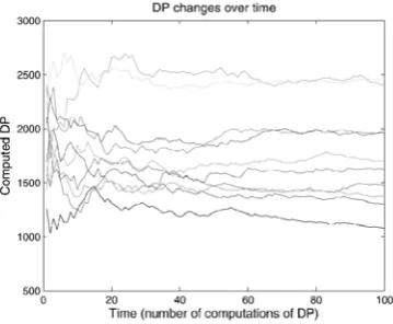
To assess the downloading similarity between a candi-date node and a neighbor, we first define the notion of download power (DP) to quantify the data access capability ofa node. The idea is that a node with higher DP is considered to be superior in downloading capability to a node with lower DP. We formulate DP for a host h as follows:

DP_h 1

jHhj

₃

Hihi:size hi:distance

₃

¼ h Xi1 h:elapse ₃H ð Þ

jH j _¼ H

Intuitively, this metric combines the metrics of download speed and distance defined in the previous section. As seen from (2), DP/download speed which is intuitive, as it captures how fast a node can download data in general. Further, we also have DP/ distance to the server which implies that for the same download speed to a server, the download power of a node is considered higher if it is more distant from the server. Consider an example to understand this relation between download power and distance. Suppose two client nodes, one in the US and one in Asia, access data from servers located in the US. Then, if the two clients show the same download time for the same object, the one in Asia might be considered to have better downloading capability for more distant servers, as the US client’s download speed could be attributed to its locality. Hence, access over greater distance is given greater weight in this metric. To minimize the effect of download anomalies and inconsistencies, we compute DP as the average across its history of downloads from all servers. Fig. 4 shows a snapshot of DP value changes for 10 sampled nodes. We can see that DP values become stable with many more observations over time. According to our observa-tions, node DP changes of greater than ₃10 percent were less than 1 percent of the whole.

Now, we define a function for neighbor estimation at host h by using information from neighbor n for object o:

NeighborEstimhðn; oÞ ¼ ₃₃₃₃ elapsenðoÞ; ð3Þ

where

₃ ¼ DPn ; ₃

¼

distance

hðserverðoÞÞ ; DP_h distance_nðserverðoÞÞ

Fig. 5. Neighbor estimation result.

and elapse_nðoÞ is the download time observed by the neighbor for the object. It is possible that the neighbor has multiple observations for the same object, in which case we pick the smallest download time as the representative.

Intuitively, to estimate the download time for object o based on the information from neighbor n, this function uses the relevant download time of the neighbor. As a rule, the estimation result is the same if all conditions are equivalent to the neighbor. To account for differences, we employ two parameters ₃ and ₃. The parameter ₃ compares the down-load powers of the node and the neighbor for similarity. If the DP of the node is higher than the neighbor, the function gives smaller estimation time because the node is considered superior to the neighbor in terms of accessibility. The parameter ₃ compares the distances to the server, so that if the distance to the server is closer for the node than the neighbor’s, the resulting estimation will be smaller.3 These correlations enable us to share observations between neighbors without any topological restrictions.

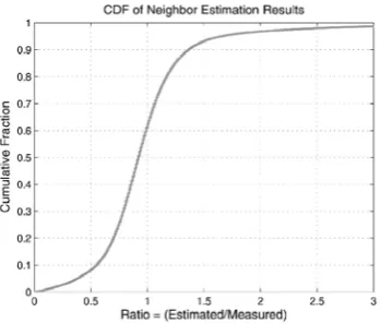
Fig. 5 illustrates the cumulative distribution of neighbor estimation results. Like the simulation in self-estimation, the estimation was made against all the actual measure-ments with a relevant observation measured in any other node. In other words, for the measured one, an estimation was attempted for every single observation that any other node measured for that object. As seen from the figure, a substantial portion of the estimated values are located near the ratio 1. Nearly 84 percent of estimations reside within a factor of 2 of the corresponding measurements. This suggests that neighbor estimation produces useful informationto rank nodes with respect to accessibility.

While neighbor estimation is useful for assessment of accessibility, multiple neighbors can provide different information for the same object. For example, if three neighbors offer their observations to a node, there can be three estimates which may have different values. Thus, we need to combine these different estimates to obtain more accurate results. We examined several combination functions, such as median, truncated mean, and weighted mean, and observed that taking the median value works well even with a small number of neighbors. Given that the number of neighbors providing relevant observations

3. We discuss how the server distance can be estimated without active probing in Section 3.4.

may be limited in many cases, we believe that taking the median should be a good choice. Hence, combining multiple estimates is done by

NeighborEstim_hðoÞ ¼ medianðNeighborEstim_hðn_i; oÞÞ; for all n_i2N0, where N0 is a subset of the neighbor set N (N0₃ N), which only includes neighbor nodes offering

NeighborEstim_hðn_i; oÞ.

We observed that combining multiple estimates with the median function significantly improves the accuracy. Although omitted due to space reasons, estimation with four neighbor observations yielded nearly 90 percent of estimates within a factor of 2, while it was 84 percent with a single neighbor observation. It becomes over 92 percent with eight neighbor observations.

To realize neighbor estimation, it is necessary to gather information from the neighbor nodes. This can be done by on-demand requests, background communications, or any hybrid form of them. Piggybacking on periodic heartbeats in the overlay network can be a practical option to save overhead.

3.4 Inferring Server Latency without Active Probing

While neighbor estimation requires latency to the server as a parameter (see (3)), we can avoid the need for active probing by exploiting the server latency estimates obtained from the neighbors themselves. If a neighbor has contacted the server, it could obtain the latency at that time by using a simple latency computation technique, e.g., the time difference between TCP SYN and SYNACK when perform-ing the download, and this latency information can be offered to the neighbor nodes. By utilizing the latency information observed in the neighbor nodes, it is possible to minimize additional overhead in estimation in terms of server location and pinging.

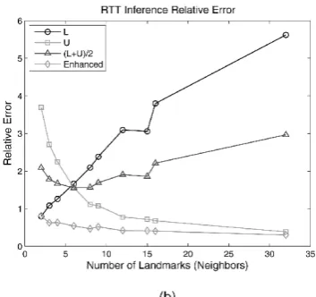
According to the study in [39], a significant portion of total paths (>90%) satisfied the property of triangle inequality. We also observed that 95 percent of total paths in our data satisfied this property. The triangulated heuristic estimates the network distance based on this property. It infers latency between peers with a set of landmarks which hold precalculated latency information between the peers and themselves [20]. The basic idea is that the latency of node a and c may lie between jlatencyða; bÞ₃latencyðb; cÞj and latencyða; bÞ þ latency ðb; cÞ, where b is one of the landmarks (b2B). With a set of landmarks, it is possible to obtain a set of lower bounds (L_A) and upper bounds (U_A). If we define L ¼ maxðL_AÞ and U ¼ minðU_AÞ, then the range ½L; U& should be the tightest stretch with which all inferred results may agree. For the inferred value, Hotz [18] suggested L because it is admissible to use A* search heuristic, while H and all linear combinations of L are not admissible. Guyton and Schwartz [19] employed ðL þ UÞ=2, and most recently, Ng and Zhang reported U performs better than the others [20].

In our system model, we can use neighbors as the landmarks because they hold latency information both to the candidate and to the object server. By applying the triangulated heuristic, therefore, we can infer the latency between the candidate and the server without probing.

Fig. 6. Latency inference results. (a) Absolute error. (b) Relative error.

However, we found that the existing heuristics are inaccurate with a small number of neighbors which may be common in our system model. Hence, we enhance the triangulated heuristic to account for a limited number of neighbors.

Our approach works by handling several situations that contribute to inaccuracy. For example, it is possible to have L > U due to some outliers, for which the triangle inequal-ity does not hold. Consider the following situation: All but one landmark give reasonable latencies, but if that one gives fairly large low and high bounds, the expected convergence would not occur, thus leading to an inaccurate answer. To overcome this problem, we remove all L_i2L_A, which are greater than U, so we can make a new range that satisfies L < U. After doing so, we observed that taking simple mean produces much better results than the existing approaches.

We also observed a problematic situation where a significant portion of the inferred low bounds suggest similar values, but high bounds have a certain degree of variance. This happens where node c is close to a but the landmarks are all apart from node a. For this, we consider a weighted mean based on standard deviations (₃). The intuition behind this is that if multiple inferred bounds suggest similar values for either low or high bounds, it is likely that the real latency is around that point. We take the weighted mean when it fails to converge due to the range being too wide, where picking any one of L, U, and ðLþ UÞ=2 is likely to be highly inaccurate. The weighted mean is defined as follows:

L ₃

₃

₃

₃

₃

₃

þ

₃

₃

₃

₃

:

ð LA þ UAÞ ð LA þ UA Þ

We report the evaluation results with the absolute error as well as the relative error for clarity. For example, if we think of two measured latencies 1 and 100 ms, and the corresponding estimations 2 and 200 ms, then these two estimations give the same picture with respect to the relative error (i.e., relative error ¼ 1 in this example). In contrast, they convey different information with respect to absolute error. In fact, 1 ms difference is usually acceptable, but 100 ms error is not for latency inference.

Fig. 6 demonstrates the inference results. As reported in [20], the heuristic employing U is overall better than the

other two existing heuristics. However, we can see that our enhanced heuristic substantially outperforms the existing heuristics with respect to both relative and absolute error metrics. In particular, the enhanced heuristic works well even when the number of landmarks is small. Since the number of neighbors which can offer the relevant latency information may be limited, the enhanced heuristic is desirable in our design. In other words, it is possible to infer the latency to the server with fairly high accuracy even in the case where only a few neighbor nodes can provide relevant information.

4 E

4.1 Experimental Setup

We conducted over 100,000 actual downloading experi-ments for a span of five months with 241 PlanetLab nodes geographically distributed across the globe. For this, we deployed a Pastry [25], [40] network, a structured overlay based on a DHT ring. We distributed data objects of four sizes: 1, 2, 4, and 8 MB, over the network, each object with a unique key. We then generated a series of random queries so that the selected nodes perform downloading the relevant objects. Table 1 provides the details of the download traces. In the simulations, we use a mixture of all traces rather than individual traces, unless otherwise mentioned.

To evaluate resource selection techniques, we design and implement a simulator which inputs the ping maps and the collective downloading traces and outputs performance results according to the selection algorithms. Initially, the simulator constructs a network in which nodes are randomly connected to each other with a predefined neighbor size without any locality or topological considerations. To

TABLE 1 Download Traces

Fig. 7. Performance over the time.

minimize error due to the construction, we repeated simulations 50 times and report the results with 95 percent confidence intervals as needed. After constructing the network, the simulator runs each resource selection algo-rithm. Initially, it constructs a virtual trace in which the list of candidates and the download time from each candidate are recorded. The candidate nodes are randomly chosen for each allocation. As the candidate may have more than one actual download record for a server, the download time is also randomly selected from them. The simulator then selects a worker based on each selection algorithm. Based on the selected worker, the download time is returned from the virtual trace.

For our evaluation, we compare the resource selection techniques based on our estimation techniques with two conventional techniques: random and latency-based selec-tions. The following describes the resource selection techniques:

. OMNI: Optimal selection; . RANDOM: Random selection; . PROXIM: Latency-based selection;

. SELF: SELF basically performs the selection by self-estimation. One exception is that it allows the node to make an estimation by partial observations if it has any observations to the object server.4 This can improve accuracy. If no estimate is available, it performs random selection;

. NEIGHBOR: NEIGHBOR performs the selection based on

neighbor estimation. If no estimate is available, it performs random selection.

4.2 Performance Comparison over Time

We begin by presenting the performance comparison over time. Fig. 7 compares the performance over the 100,000 consecutive job allocations. As the default, we set both the candidate size and the neighbor size to 8 (and it is applied to all the following experiments, unless otherwise mentioned). Overall the proposed techniques yield good results: SELF is the best across time and

NEIGHBOR works better than PROXIM most of the time. RANDOM

yields poor performance

sizeðoÞ

4. This is done by a simple statistical estimator: DownSpeedhðsÞ , where

DownSpeedhðsÞ stands for the mean download speed from the node to the

server.

with a significant degree of variation, as expected. PROXIM is about three times of optimal with a relatively high degree of variation compared to the suggested techniques. SELF works best approaching about 1.4 of optimal at the end of the simulation. This shows that simple consideration of past access behavior in addition to latency greatly benefits to choose a good candidate.

NEIGHBOR is poor at first, but outperforms PROXIM after

about 6,000 simulation time steps. This is because there may be many more chances of random selection at first stage; after warming up, however, it exploits neighbor observations, leading to better performance. Nonetheless, NEIGHBOR shows a noticeable gap to SELF. This can be explained mainly by the hit rate on the number of relevant observations from the neighbors; we observed that the average number of observations was around 2 even at the end of the simulation, while neighbor estimation yields stable results with more than four observations, as discussed in Section 3.3. Thus, NEIGHBOR could perform better with a higher hit rate; improving hit rate is part of our future work.

4.3 Impact of Candidate Size

In our system model, a set of candidate nodes is evaluated for its accessibility before allocating a job. We now investigate the impact of candidate size (jCj). Fig. 8 demonstrates the performance changes with respect to candidate size. In Fig. 8a, mean ratio to optimal increases along the candidate size. This is because OMNI has many more chances to see better candidates to choose from, resulting in the larger performance gaps. Nonetheless, we can see that the suggested techniques work better with many more candidates, making the slopes gentle compared to the conventional ones. Fig. 8b compares mean download time for the selection techniques. As seen in the figure, SELF continues to produce diminished elapsed times as the candidate size increases, yielding the best results among selection techniques.

NEIGHBOR follows SELF with con-siderable gaps against the

conventional techniques. Inter-estingly, PROXIM shows unstable results with greater fluctuation than RANDOM over the candidate sizes. This result indicates that the proposed techniques not only work better than conventional ones across candidate sizes, but also further improve as the candidate size increases.

4.4 Impact of Neighbor Size

We next investigate the impact of neighbor size on NEIGHBOR

(the other heuristics are not affected by this parameter). Fig. 9 shows how the selection techniques respond across the number of neighbors (jNj). As can be seen in the figures, increasing the neighbor size dramati-cally improves the performance, while the others make no changes as expected. For example, the average download time in jNj ¼16 is dropped to about 70 percent of the time for jNj ¼2. The ratio to optimal is also dropped from 4.0 at jNj ¼ 2 to 2.6 at jNj ¼ 16. This is because it has morechances to obtain relevant observations with many more neighbors, thus decreasing the possibility of random selection. This result suggests that NEIGHBOR will work better in environments where the node has connectivity with a greater number of

Fig. 8. Impact of candidate size. (a) Mean ratio to optimal. (b) Mean download elapsed time.

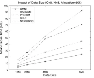
4.5 Impact of Data Size

We continue to investigate how the selection techniques work over different data sizes. Since the size of accessed objects can vary depending on applications in reality, selection techniques should work consistently across a range of data sizes. In this experiment, we run the simulation with individual traces rather than the mixture of the traces. In Fig. 10, we can see linear relationship between data size and mean download time. However, each technique shows a different degree of slope: SELF

and NEIGHBOR increase more gently than the conventional heuristics. With simple calculation, the slopes (i.e., ₃y=₃x) of the techniques are RANDOM = 10.9, PROXIM = 8.1, SELF = 3.8, and

NEIGHBOR = 5.1. This result implies that the proposed

techniques not only work consistently across different data sizes, but they are also much more useful for data-intensive applications.

4.6 Timeliness

While it is crucial to choose good nodes for job allocation, it is also important to avoid bad nodes when making a decision. For instance, selecting intolerably slow connec-tions may lead to job incompletion due to excessive downloading cost or time-outs. However, it is almost impossible to pick good nodes every time because there are many contributing factors.

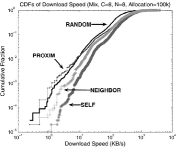
We observed how many times the techniques choose slow connections. Fig. 11 shows the cumulative distributions of the speed of connections with log-log scales, and we can see that the proposed techniques more often avoid slow connections. SELF

most successfully excludes low-speed connections, and

NEIGHBOR also performs better than the conventional techniques.

When we count the number of poor connections selected, SELF

chose connections under 5 KB/s less than 30 times,while PROXIM

made more than 290 selections, which is almost an order of magnitude larger than SELF. One interesting result is that PROXIM

selects poor connections more frequently than RANDOM (293 and 194 times, respec-tively). This implies that relying only on latency information alone greatly increases the chance of very poor connections, thus leading to unpredictable response time. Compared to this, our proposed techniques successfully reduce chances to choose low speed connections by taking accessibility into account.

4.7 Multiobject Access

Many distributed applications request multiple objects [41], which means that a job of such applications accesses more than one object to complete the task. For example, bioinformatics applications such as BLAST [15] repeatedly access remote gene databases to compare patterns. We conducted experiments to see the impact of multiobject access. Fig. 12 shows the results where jobs require to access

Fig. 11. Cumulative distribution of download speed. Fig. 12. Multiobject access.

multiple objects. As can be seen in the figure, the ratio to optimal gradually decreases with increasing number of objects for all selection techniques. This is because even optimally selected nodes may not have good performance to some objects, resulting in greatly increased download times. SELF and NEIGHBOR not only consistently outper-form the conventional techniques over the number of objects, but they also approach optimal (ratio = 1.24 and 1.55 when the number of objects is 8). To sum it up, the suggested techniques also work better than the conven-tional techniques for multiobject access.

4.8 Impact of Churn

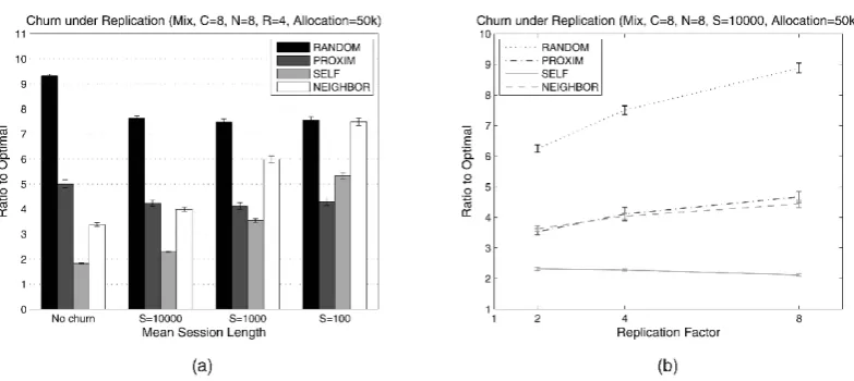
Churn is prevalent in loosely coupled distributed systems. To see the impact of churn, we assume that mean session lengths of nodes are exponentially distributed. In this context, the session length is equivalent to the simulation time. For example, if the session length of a node is 100, the node changes its status to inactive after 100 simulation time steps. The node then joins again after another 100 time steps. We assume that nodes lose all past observations when they change status. Therefore, churn will have a greater impact on our selection techniques because we rely on historic observa-tions. In contrast, the conventional techniques suffer little from churn since they do not have any dependence on past observations. The virtual trace excludes objects for which the relevant servers are inactive. We tested three mean session lengths: s¼100, s¼1;000, and s¼10;000, corresponding to extreme, severe, and light churn rates, respectively.

Fig. 13 illustrates the impact of churn. As mentioned, there is little impact on conventional techniques, while our techniques are degraded in performance due to loss of observations. In Fig. 13a, SELF is comparable to PROXIM even under extreme churn.

NEIGHBOR degrades and becomes worse than PROXIM under

severe churn (s¼1;000). This is because NEIGHBOR is likely to fail to collect the relevant observations, thus relying more on random selection, while SELF can perform reasonably accurate estimation with only a dozen of observations. Nonetheless,

NEIGHBOR still works better than PROXIM in light churn (s ¼

10;000) with lower overhead. Fig. 13b explains why NEIGHBOR

suffers under severe and extreme churn. In the figure, the neighbor estimation rate means the fraction that NEIGHBOR

success-fully estimates based on neighbor estimation rather than random selection. Under light churn, the neighbor estimation

rate is still over 90 percent, but it drops to 60-70 percent in severe churn, implying that 30-40 percent of the decisions have been made by random selection. Under extreme churn, the neighbor estimation rate drops below 10 percent, so it essentially reduces to

RANDOM.

To summarize, the proposed techniques are fairly stable under churn in which nodes suffer from loss of observations. The result shows that SELF is comparable to

PROXIM even under extreme churn, while NEIGHBOR is

comparable to PROXIM when churn is light.

4.9 Impact of Replication

In loosely coupled distributed systems, replication is often used to disseminate objects to provide locality in data access as well as high availability. We investigate the impact of replication to see if the proposed techniques consistently work in replicated environments.

For this, we construct replicated environments in which same-sized objects in the traces are grouped according to the replication factor and the object in the group is considered as a replica. The virtual trace is then constructed based on the group of the objects. In detail, for all objects in the group, a randomly selected download time from each candidate is recorded in the virtual trace. The simulator then returns the download time according to the selected candidate and the replica server.

RANDOM will work the same as in no-replication environment

with a random function to choose both a candidate and a replica server. PROXIM measures latencies from every candidate to every server, and then the pair with the smallest latency will be selected. SELF is similar to PROXIM: each candidate calculates the accessibility for each server and reports the best one. In the case

of NEIGHBOR, the candidate gathers all the relevant information

from the neighbors. If it finds more than one server, Neighbor EstimðoÞ function is performed against each server, andthen the best one is reported to the initiator. For both SELF and

NEIGHBOR, the initiator finally selects the candidate with the best

accessibility.

Fig. 14 shows performance changes across replication factors (jRj). It is likely that the performance of all selection techniques improve as the replication factor increases because of data locality, and the result agrees with this expectation, as shown in Fig. 14b. PROXIM has significantly diminished mean download time (nearly half) under

Fig. 13. Impact of churn. (a) Mean download elapsed time. (b) Neighbor estimation rate.

replication, but it is still worse than the proposed techniques. SELF and NEIGHBOR outperform the conven-tional techniques over all the replication factors. In Fig. 14a, we can see that SELF

further reduces ratio to optimal as replication factor increases, while the others increase. NEIGHBOR widens the gap against conventional techniques with increasing replication factor.

Next, we investigate the impact of churn in replicated environments. First, we fix the replication factor at 4, and observe the performance change over a set of mean session lengths. As can be seen in Fig. 15a, the results are fairly similar with the ones under churn in the nonreplicated environment. However, SELF is a little worse than PROXIM under extreme churn. NEIGHBOR is comparable to PROXIM under light churn, but degrades under severe and extreme churn as in no replication. Then we investigate performance sensitivity to the replication factor under light churn (i.e., s ¼ 10,000). As seen in Fig. 15b, SELFis much better than PROXIM across all replication factors. NEIGHBOR is fairly comparable to PROXIM under light churn despite greater chance of random selection.

To summarize, the proposed selection techniques consistently

outperform the conventional techniques in replicated environ-ments. The results under churn are fairly consistent with the results

without replication: SELF is comparable to PROXIM

under severe churn and NEIGHBOR is comparable to PROXIM

under light churn.

5 R

W

5.1 Resource Discovery and Allocation

The work on resource discovery and allocation is closely related to ours. Condor [42] provides a matchmaking framework which provides a stateless matching service. In [7], the authors presented a decentralized matchmaking based on aggregation of resource information and Content Addressable Network (CAN) routing [24]. The Cluster Computing on the Fly (CCOF) project [8] seeks to harvest CPU cycles by using search methods in a peer-to-peer computing environment. SWORD [27] provides distributed resource discovery by a multiattribute range search against a DHT on which the periodic measures of each node are stored. All these techniques focused more on per-node characteristics of individual nodes, e.g., CPU, memory, disk space, network interface, etc. In contrast, our approach is more interested in pairwise characteristics for the resource selection with considerations of impact on end-to-end data access. SWORD [27] provides network coordinates as the location information by using Vivaldi [37], but the latency is not sufficient for bandwidth-demanding applications.

Fig. 14. Performance under replicated environments. (a) Mean ratio to optimal. (b) Mean download elapsed time.

Fig. 15. Impact of churn under replication. (a) Replication factor = 4. (b) Mean session length ¼ 10,000 (light churn).

5.2 Network Performance Estimation

Much research has been carried out in network perfor-mance estimation for selection problems over the past decade. To infer network performance, many estimators were employed. Some research in [35], [43], [44], [45] focused on estimating available bandwidth, the minimum available bandwidth of the links along a path. Predicting RTT [20], [37], [46], [47], [48] has also been extensively studied because it is a widely used metric in the Internet today. TCP throughput [49], [50], [51] is also a frequently used metric for network performance. In this paper, we employ accessibility to quantitatively determine data access capability between a pair of nodes.

Network performance estimation techniques fall into three classes with respect to the measurement methods: active probing, partial probing, and passive observing. Active probing injects a chain of packets to measure the network performance. Thus, the estimation is often believed fairly accurate based on current network conditions, but it requires not only time delay but also incurs additional traffic overhead for the actual measurement. Meanwhile, many latency prediction techniques uses partial probing. These techniques infer latency of n2 pairs by OðnÞ probing. However, as latency may not be directly correlated to network bandwidth, selections relying only on latency can mislead bandwidth-demanding applications. Passive techniques utilize past collected observations for the estimation. This approach is attractive because it makes a timely prediction with little additional traffic. However, existing techniques are limited by topological regions (e.g., LANs or IP prefixes) for sharing observations. In contrast to this, our passive estimation technique, neighbor estimation, has no such topological or geographical constraints, and yields good accuracy, sufficient for the selection problems to which it has been applied.

6 C

Accessibility is a crucial concern for an increasing number of data-intensive applications in loosely coupled distributed systems. Such applications require more sophisticated resource selection due to bandwidth and connectivity unpredictability. In this paper, we presented decentralized, scalable, and efficient resource selection techniques based on accessibility. Our techniques rely only on local, historic

observations, so it is possible to keep network overhead tolerable. We showed that our estimation techniques are sufficiently accurate to provide a meaningful rank order of nodes based on their accessibility. Our techniques outper-form conventional approaches and are reasonably close to the optimal selection. In particular, the self-estimation-based selection approached 1.4 of optimal over time, the neighbor estimation-based selection was within 2.6 of optimal with 16 neighbors, compared to a proximity-based selection that was over three times the optimal. With respect to the mean elapsed time, the self- and neighbor-estimation-based selections were, respectively, 52 and 70 percent more efficient than proximity-based selection. We also investi-gated how our techniques work under node churn and showed that they work well under churn circumstances in which nodes suffer from loss of observations. Finally, we showed that our techniques consistently outperform conventional techniques in replicated environments.

In this work, we focused on performance for the accessibility metric. The next step is to capture availability as well as performance to take dynamism into account. In addition to this, we plan to extend our work by providing system-wide dissemination of observations so that the node has more chances to see relevant observations in estimation. This is reasonable since neighbor estimation has no constraints on topological or geographical similarities to utilize observations coming from other nodes.

R

[ 1] D.P. Anderson and G. Fedak, “The Computational and Storage Potential

of Volunteer Computing,” Proc. IEEE Int’l Symp. ClusterComputing

and the Grid (CCGRID ’06), pp. 73-80, 2006.

[2] A. Haeberlen, A. Mislove, and P. Druschel, “Glacier: Highly Durable,

Decentralized Storage Despite Massive Correlated Fail-ures,” Proc.

Symp. Networked Systems Design and Implementation(NSDI ’05), May 2005.

[3] J. Kubiatowicz, D. Bindel, Y. Chen, P. Eaton, D. Geels, R. Gummadi, S. Rhea, H. Weatherspoon, W. Weimer, C. Wells, and B. Zhao,

“Oceanstore: An Architecture for Global-Scale Persistent Storage,”

Proc. ACM Int’l Conf. Architectural Support for Programming Languages and Operating Systems (ASPLOS ’07), Nov. 2000.

[4] R. Bhagwan, K. Tati, Y.-C. Cheng, S. Savage, and G.M. Voelker, “Total Recall: System Support for Automated Availability

Management,” Proc. Symp. Networked Systems Design and

Imple-mentation (NSDI ’04), p. 25, 2004.

[5] A. Chien, B. Calder, S. Elbert, and K. Bhatia, “Entropia: Architecture

and Performance of an Enterprise Desktop Grid System,” J. Parallel

and Distributed Computing, vol. 63, no. 5 pp. 597-610, 2003.

[6] D. Kondo, A.A. Chien, and H. Casanova, “Resource Management for

Rapid Application Turnaround on Enterprise Desktop Grids,”

Proc. ACM/IEEE Conf. Supercomputing (SC ’04), p. 17, 2004.

[7] J.-S. Kim, B. Nam, P. Keleher, M. Marsh, B. Bhattacharjee, and

A. Sussman, “Resource Discovery Techniques in Distributed Desktop

Grid Environments,” Proc. IEEE/ACM Int’l Conf. GridComputing

(GRID ’06), Sept. 2006.

[8] D. Zhou and V. Lo, “Cluster Computing on the Fly: Resource Discovery

in a Cycle Sharing Peer-to-Peer System,” Proc. IEEE Int’l Symp.

Cluster Computing and the Grid (CCGRID ’04), pp. 66-73, 2004.

[9] D.P. Anderson, J. Cobb, E. Korpela, M. Lebofsky, and D. Werthimer,

“Seti@home: An Experiment in Public-Resource Computing,” Comm.

ACM, vol. 45, no. 11, pp. 56-61, 2002.

[10] “Search for Extraterrestrial Intelligence (SETI) Project,” http:// setiathome.berkeley.edu, 2009.

[11] “BOINC: Berkeley Open Infrastructure for Network Computing,” http://boinc.berkeley.edu/, 2009.

[12] “PPDG: Particle Physics Data Grid,” http://www.ppdg.net, 2009.

[13] N. Massey, T. Aina, M. Allen, C. Christensen, D. Frame, D. Goodman, J. Kettleborough, A. Martin, S. Pascoe, and D. Stainforth, “Data Access and Analysis with Distributed Federated Data Servers in

climateprediction.net,” Advances in Geosciences, vol. 8,

pp. 49-56, June 2006.

[14] G.B. Berriman, A.C. Laity, J.C. Good, J.C. Jacob, D.S. Katz, E. Deelman, G. Singh, M.-H. Su, and T.A. Prince, “Montage: The Architecture and Scientific Applications of a National Virtual Observatory Service for Computing Astronomical Image Mosaics,”

Proc. Earth Sciences Technology Conf., 2006.

[15] “BLAST: The Basic Local Alignment Search Tool,” http:// www.ncbi.nlm.nih.gov/blast, 2009.

[16] W. Hoschek, F.J. Jae´n-Martı´nez, A. Samar, H. Stockinger, and

K. Stockinger, “Data Management in an International Data Grid

Project,” Proc. IEEE/ACM Int’l Conf. Grid Computing(GRID ’00),

pp. 77-90, 2000.

[17] Y.-M. Teo, X. Wang, and Y.-K. Ng, “Glad: A System for Developing

and Deploying Large-Scale Bioinformatics Grid,” Bioinformatics, vol.

21, no. 6, pp. 794-802, 2005.

[18] S. Hotz, “Routing Information Organization to Support Scalable Interdomain Routing with Heterogeneous Path Requirements,” PhD dissertation, 1994.

[19] J.D. Guyton and M.F. Schwartz, “Locating Nearby Copies of Replicated

Internet Servers,” SIGCOMM Computer Comm. Rev., vol. 25, no. 4,

pp. 288-298, 1995.

[20] E. Ng and H. Zhang, “Predicting Internet Network Distance with

Coordiantes-Based Approaches,” Proc. IEEE INFOCOM ’02,

pp. 170-179, 2002.

[21] E. Cohen and S. Shenker, “Replication Strategies in Unstructured

Peer-to-Peer Networks,” Proc. ACM SIGCOMM ’02, pp. 177-190, 2002.

[22] Q. Lv, P. Cao, E. Cohen, K. Li, and S. Shenker, “Search and Replication

in Unstructured Peer-to-Peer Networks,” Proc.ACM SIGMETRICS

’02, pp. 258-259, 2002.

[23] I. Stoica, R. Morris, D. Karger, M.F. Kaashoek, and H. Balakrishnan, “Chord: A Scalable Peer-to-Peer Lookup Service for Internet

Applications,” Proc. ACM SIGCOMM ’01, pp. 149-160, 2001.

[24] S. Ratnasamy, P. Francis, M. Handley, R. Karp, and S. Schenker, “A

Scalable Content-Addressable Network,” Proc. ACM SIG-COMM ’01,

pp. 161-172, 2001.

[25] A. Rowstron and P. Druschel, “Pastry: Scalable, Distributed Object

Location and Routing for Large-Scale Peer-to-Peer Sys-tems,” Proc.

IFIP/ACM Int’l Conf. Distributed Systems Platforms(Middleware ’01), pp. 329-350, Nov. 2001.

[26] B. Zhao, L. Huang, J. Stribling, S. Rhea, A. Joseph, and J. Kubiatowicz, “Tapestry: A Resilient Global-Scale Overlay for Service Deployment,”

IEEE J. Selected Areas in Comm., 2003.

[27] D. Oppenheimer, J. Albrecht, D. Patterson, and A. Vahdat, “Design and

Implementation Tradeoffs for Wide Area Resource Discovery,” Proc.

Int’l Symp. High Performance Distributed Comput-ing (HPDC),

2005.

[28] “PlanetLab,” http://www.planet-lab.org, 2009.

[29] S.G. Dykes, K.A. Robbins, and C.L. Jeffery, “An Empirical Evaluation

of Client-Side Server Selection Algorithms,” Proc. IEEEINFOCOM

’00, pp. 1361-1370, 2000.

[30] Using Using Data Accessibility for Resource Selection in Large-Scale Distributed Systems, IEEE Conference, June 2009.

A

Bachina Anusha Revieved B.Tech in 2008. She is pursuing M.Tech in QIS College of Engineering & Technology, Ongole.She is very interested in Distributed systems and Netwoking.

VENKATA SUBBAREDDY PALLAMEDDY received M.E degree in Computer Science & Engg in 2007. His Research Areas are Data Ming, Networking, Data ware housing and Artificial Intelligence.He has published large number of papers in different National & International Conferences and International journals . He is Editorial

Board Member for International Journal of Computer Technology and Applications (IJCTA), International Journal of Computer Trends and Technology (IJCTT), International Journal of Engineering Trends and Technology (IJETT) and Technical reviewer of many International journals. He is a member of International Association of Engineers, IACSI and ISTE.

T.V.Sai Krishna Received His M.Tech From JNTU in 2007.He is currently Research Scholar of JNTU Kakinada.His Research Areas are data mining ,Data Ware housing & Image Processing.