Study on the impulsive pressure of tank oscillating by force towards multiple degrees of freedom

(1)

Study on the impulsive pressure of tank oscillating by force

towards multiple degrees of freedom

Shigeyuki Hibi1,*

1_{The National Defense Academy, Department of Mechanical Systems Engineering, 1-10-20 Hashirimizu,} Yokosuka, Kanagawa 239-8686, Japan

Abstract. Impulsive loads should be excited under nonlinear phenomena with free surface fluctuating severely such as sloshing and slamming. Estimating impulsive loads properly are important to recent numerical simulations. But it is still difficult to rely on the results of simulations perfectly because of the nonlinearity of the phenomena. In order to develop the algorithm of numerical simulations experimental results of nonlinear phenomena are needed. In this study an apparatus which can oscillate a tank by force was introduced in order to investigate impulsive pressure on the wall of the tank. This apparatus can oscillate it simultaneously towards 3 degrees of freedom with each phase differences. The impulsive pressure under the various combinations of oscillation direction was examined and the specific phase differences to appear the largest peak values of pressure were identified. Experimental results were verified through FFT analysis and statistical methods.

1 Introduction

Impulsive loads[1,2] should be excited under nonlinear phenomena with free surface fluctuating severely such as sloshing and slamming in the field of naval architecture. Many studies about not only the estimation of the impulsive loads but also elastic behavior of structures have been carried out along with the recent developments of the numerical simulation methods. However the number of experiments to verify those numerical techniques is not enough because of the nonlinearity of the phenomena.

In this study an apparatus which can oscillate a tank by force was introduced in order to investigate impulsive pressure on the wall of the tank. This apparatus can oscillate it simultaneously towards 3 degrees of freedom (up-down, left-right and rotation) with each phase differences. It could happen that larger impulsive pressure is excited under oscillating the tank simultaneously towards multiple degrees of freedom than under single direction oscilation. The author examined the impulsive pressure under the various combinations of oscillation direction and identified the specific

phase differences to appear the largest peak values of pressure. Therefor the author showed larger impulsive pressure could appear under the oscillation towards multiple directions in comparison with the oscillation towards a single direction.

In the meantime the uncertainty of the result of experiments has been settled by the GUM[3] (Guide to the Expression of Uncertainty in Measurement) since 1993. Based on this a FFT analysis about measured pressure values was carried out and the confidence interval of them

based on t-distribution was also determined. At

last uncertainty analysis based on the GUM was executed and the reliability of the experiment was assured.

2 Experimental apparatus and

measuring instruments

2.1 Specification of oscillation apparatus

(2)

The size of tank is 400400100 (mm)

(Height WidthDepth).

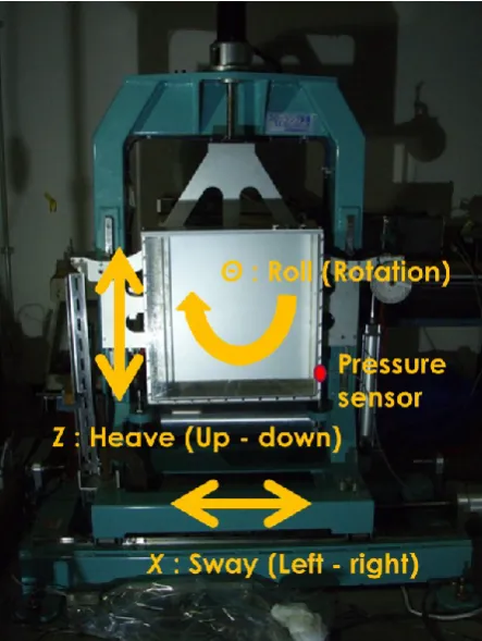
We define the symbols for the oscillation directions of 3 degrees of freedom as follows in Fig.2. Heave oscillation (Up – down) stands for Z and Sway oscillation (Left – right) stands for

X and Roll oscillation (Rotation) stands for .

Fig. 1. Oscillation apparatus with 3 degrees of freedom.

Fig. 2. Oscillation direction and pressure sensor position.

Table 1. Specification of the apparatus about oscillation.

Direction of

oscillation Maximum amplitude Minimum period

Heave (Z)

(Up-down) 50 mm 1.0 sec. Sway (X)

(Left-right) 50 mm 1.0 sec.

Roll ()

(rotation) 45 deg. 1.0 sec.

2.2 Measuring instruments

(1) Potentiometer

In order to confirm the acculacy of the roll oscillation control of a servo motor a potentio-meter is attached to measure a rotation angle at every moment.

(2) Laser displacement gauge

In order to confirm the acculacy of both heave and sway oscillation control of servo motors laser displacement gauges are placed to measure displacements at every moment.

(3) Pressure sensor

A pressure sensor is attached on the right side of the tank mounted on the apparatus. The position of the sensor is 40mm from the bottom. The pressure receiver is a round with a diameter of 8mm.

3Analytical methods for measured data

3.1. FFT (Fast Fourier Transform)analysis

A FFT analysis are applied to the measured pressure data of time history in this study. Frequency components including in each data wave profile are discussed.

3.2 Determining the confidence intervals based on the t-distribution

Independent randam variables subject to the normal distribution X1, X2, ... XN are assumed

that mean values are  and variances are _2

(usually unkonwn). Then sample mean X and

unbiased variance _u2 _{are defined by eq. (1).}



 

 



 N

i i

N

i i

X X N

u X N X

1

2 2

1 1 ( )

1 ,

(3)

Then randam variable T defined by eq. (2) is

subject to Student’s t – distribution of N −1

degree of freedom.

T



X 



/



u/ N



(2)

Probability density function of the t –

distri-bution fN1

 

t is given by eq. (3).

 





2 / 2

1 1 ₁

2 1 1

2 N

N _N _Nt

N N t f                             (3)

Here is the gamma function.

Therefore in case of a sample of size N the

confidence interval at a confidence level z % is

given by eq. (4).

N u z t x N u z t

x N1( %)    N1( %) (4)

3.3 Uncertainty analysis

Uncertainty about measuring according to the GUM guidance is evaluated as follows. First of all we determine factors of dispersion in the measuring procedure.

There are 2 types of methods for the estimation of uncertainty in the GUM guidance. One is called ‘A’ type of uncertainty. Its type is based on a statistical method. We estimate uncertainty of each factor using mean values and standard deviations in this type of uncertainty.

The other is called ‘B’ type of uncertainty. Its type is based on another method (e.g. technical information or some experience) without a statistical approach.

After we select the dispersion factors into 2 types of uncertainty, we combine the result to estimate the total uncertainty. the expanded

uncertainty U is obtained by multiplying the

combined standard uncertainty uc(y) by a

coverage factor k (k = 2. This means the 95%

confidence level).

4 Experiment and discussion

4.1 Investigating phase differences during simultaneous oscillation towards 2 degrees of freedom

The reliability of oscillation amplitude towards each degree of freedom is assured even with a period close to the natural period of the tank by previous study.

In this study we chose 3 pairs of 2 degrees of freedom from 3 one. Those will be subscribed

as follows ( X,  Z, XZ). The oscillation

period is uniformly 1.08 (sec.) which is close to the natural period of the tank in case of the water depth is 60 mm (fixed). The oscillation

amplitudes are 15 mm for X and Z and 20

degrees for .

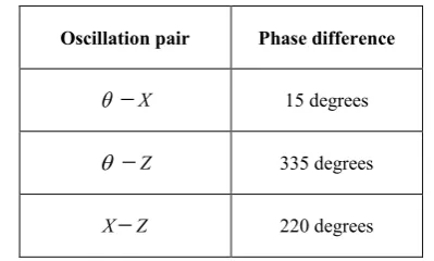
We measured time historys of pressure on the wall of the tank repeatedly while changing the phase difference from 0 degree to 360 degrees. We identified the phase difference which cause the largest peak value of pressure for each oscillation pair ( X,  Z, XZ).

The results are shown in Table 2.

Table 2. Phase difference which cause the largest peak value.

Oscillation pair Phase difference

 X 15 degrees

 Z 335 degrees

XZ 220 degrees

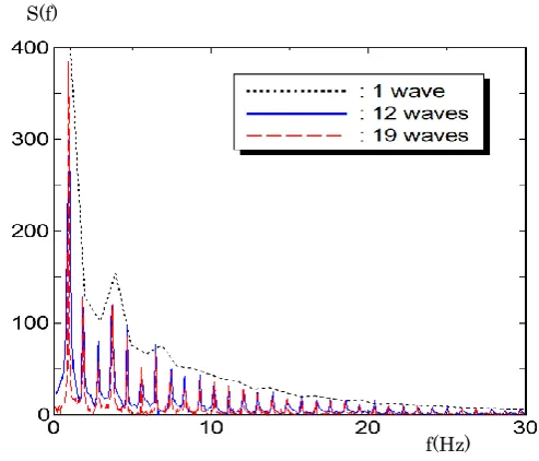
Example results of time history of pressure for each oscillation pair are shown in Figs. 3(a), (b) and (c). In any cases it can be deduced that there is periodicity in the pressure fluctuation, but it is found that the peak values have variations.

4.2 FFT analysis for measured time history of

pressure

(4)

interval contains the ones for 12 and 19 period intervals. We can also deduce that although the obtained

peak values varies, the waveform itself seems periodic.

Fig. 3(a).Time history of pressure about  X oscillation.

Fig. 3(b).Time history of pressure about  Z oscillation.

Fig. 3(c).Time history of pressure about XZ oscillation.

Fig. 4(a).FFT analysis about  X oscillation.

Fig. 4(b).FFT analysis about  Z oscillation.

Fig. 4(c).FFT analysis about XZ oscillation. p (Pa)

p (Pa)

S(f) S(f)

S(f)

f(Hz)

(5)

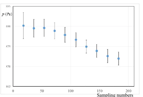
4.3 Estimation of confidence intervals for the confidence level 95%

Experiments were repeated as one measurement for 20 seconds. Peak values were extracted from the time history of pressure for each oscillation pair. Next confidence intervals for the confidence level 95 % were determined. The results are shown in the Fig. 4.

Although the width of the confidence interval tends to decrease when the number of samples increases, it is considered that there is a significant width, which may indicate the nonlinearity of the present experimental data.

Fig. 5(a). Estimation of peak values at confidence level 95% about  X oscillation.

Fig. 5(b). Estimation of peak values at confidence level 95% about  Z oscillation.

Fig. 5(c). Estimation of peak values at confidence level 95% about XZ oscillation.

4.4 Determining the expanded uncertainty

Expanded uncertainty was determined according to the budget table shown in Table 3.

The function fused to estimate the uncertainty

when measuring pressure values is in eq. (5).

_f ___g_a__V₍_d₎__V₍₂₀₎_ (5)

Where  is the density of water and g is the

gravitational acceleration. ‘a’ is the coefficient for conversion from voltage to pressure. V(d) is the voltage value of an amplifier at the d mm water depth and V(20) is the voltage value of an amplifier at the 20 mm water depth.

The expanded uncertainty calculated from Table 3 is 101.9 (Pa). The number of iterations used here is 11 times. In most cases it can be seen that the peak value varies around a mean value at this interval.

5 Conclusion

In this study impulsive pressure on the tank wall were measured and some information were found about it as below.

・ The fluctuation measured had some

periodism but the peak values had variation.

・From the estimation of confidence intervals

for the measured values at the confidence level 95% significant intervals were found to exist.

・Since characteristics of impulsive pressure

for the oscillation directions of 2 degrees of freedom is known, confirmation of that for the oscillation directions of 3 degrees of freedom is a future task.

Sampling numbers

(6)

References

1. Hakan Akyildiza, Erdem U¨nal, Ocean Engineering

32, 1503 (2005)

2. P. Temarel, W. Bai, A. Bruns, Q. Derbanne, D. Dessi,S. Dhavalikar, N. Fonseca, T. Fukasawa, X. Gu, A. Nestegård,A. Papanikolaou, J. Parunov, K.H. Song m, S. Wang, Ocean Engineering 119, 274 (2016)

3. JCGM2008, Evaluation of measurement data - Guide to the expression of uncertainty in measurement, (2008)

Table 3. Budget table for the estimation of uncertainty

Cause of

uncertainty uncertaintyType of probabilistic distributionShapes of MeanvalueSensitivityfactor uncertaintyStandard

Coefficient for conversion

from voltage to pressure Repeated experiment A Normal 159.0 3.888 0.8828 Voltage value at the

20mm water depth Repeated experiment A Normal 2.815 1558 0.03199 Calibration of

the pressure sensor Calibration error ofthe pressure sensor B Uniform 2.418 1 4.35 Calibration of

the amplifier Calibration errorof the amplifier B Uniform 5.00 1 9.00 Combined

standart uncertainty 50.96(Pa)

Expanded

uncertainty 101.9(Pa)

Factors of uncertainty :

a

 20

V

2 / 2 0pdt



Vp

c

u

i

xf  

Vamp

u

x

i