Vol. 4, Issue 5, May 2015
Data Mining Techniques with a Case Analysis
Using Clementine
Sathish.S.N
Project Manager, Infosys Limited, Mysore, India
ABSTRACT: This paper aims to explain the concept of Data Mining features by taking a case study/project for analysis.
KEYWORDS: Data Mining; Data Warehouse; Clementine; Association Rule; SPSS I. INTRODUCTION
Introduction to Case:
This case is about analyzing crimes which was recorded a stored in a data file. Objective of the case analysis is to find the following:
Explore data and explain patterns in “volume” crimes
Find related crimes which seem to have been committed by the same offender Find related crimes even if they are widely distributed in time and geography
Introduction to Data:
The fictional crime reports used for the demo consist of 662 crimes (rows) which has taken place in a city. Each record contains 46 fields. These data are available in a .csv file. Let’s look at the fields which will go through analysis.
Field Name Description of Field Crime Report Information – Reference, Time & Place
Crno Crime Reference Number
Date Date of Crime Report
Day Day of Week
Time Time of Day
GridRef Grid Reference of Crime Location – X & Y combined
Modus Operandi (MO) – Features of Method
MOentry Method of entry to premises – break-in, artifice etc.
MOpoint Point of entry to premises
MOsec Security features – alarmed, locked, unlocked, open
MOalarm Method of dealing with alarm if any – disabled, evaded, not set, etc.
MOpose Who did the offender pose as (where applicable) in order to gain entry
MOexit Was a point of exit prepared? (Y/N)
MOdoorsec Was the door secured? (Y/N)
MOtidy Did the offender perform a tidy search? (Y/N)
Vol. 4, Issue 5, May 2015
MOcontain Did the offender take a container (e.g. bag or suitcase) (Y/N)
MOentfea Features of entry to premises (e.g. smashed lock)
Property Stolen or Damaged
Paud Audio equipment
Pvid Video equipment
Pcomp Computer equipment
Pfur Furs
Pmoney Cash
Pchqcrd Cheque card or credit card
Pmed Medicines
Pphone Telephones
Pclock Clocks
Pcalc Calculators
Palch Alcoholic beverages
Prec Music recordings
Pjewel Jewellery
Ppurse Purse or wallet
Pdoor Door damaged
Pwind Window damaged
Pcashpnt Cash-point or “hole in the wall machine” damaged
Pvend Vending machine damaged
Pphonebox Phone box damaged
Pstrfurn Street furniture damaged
Crime Classification
HOcode Code indicating type of crime as used by Police forces & Home Office
Short Description Description of type of Crime e.g. Burglary, theft from person etc.
Derived Fields
Hour Hour of day (0-23)
DayNum Day of week as a number (1-7)
MonthNum Month of year as a number (1-12)
DayOfMonth Day of month
DayOfYear Day of year (0-364)
GridX Grid reference X component
GridY Grid reference Y component (negated so that plot give map orientation)
MonthStr Month number expressed as a string
Vol. 4, Issue 5, May 2015
Crime Report Information
o Ref no., date, time, day of week, grid reference of location Modus Operandi
o Method of entry, point of entry, security features, method of dealing with alarm, what the offender posed as etc.
Property stolen or damaged
o Audio equipment, video equipment, computer, purse etc.
Other
o Home Office code, short description
II. STREAM
Streams are created by drawing diagrams of data operations relevant to your business on the main canvas in the interface. Each operation is represented by an icon or node, and the nodes are linked together in a stream representing the flow of data through each operation.
Based on the case, we have designed the below stream:
Vol. 4, Issue 5, May 2015
Nodes Node Names Node Usage
Variable File Node A Variable File node, which you set up to read the data from the data source. It reads data from delimited column text file. For example reading data from .CSV file.
Table Node The Table node displays the data in table format, which can also be written to a file. This is useful anytime that you need to inspect your data values or export them in an easily readable form.
Plot Node The Plot node shows the relationship between numeric fields. You can create a plot by using points (a scatter plot) or lines.
Distribution Node The Distribution node shows the occurrence of symbolic values, such as mortgage type or gender.
Histogram Node The Histogram node shows the occurrence of values for numeric fields. It is often used to explore the data before manipulations and model building.
Filter Node The Filter node filters (discards) fields, renames fields, and maps fields from one source node to another.
Select Node The Select node selects or discards a subset of records from the data stream based on a specific condition. For example, you might select the records that pertain to a particular sales region.
Analysis:
1. Figure 1 and 2 below shows the percentage (%) and the count of various types of crimes done from the dataset.
Node used for this is:
Vol. 4, Issue 5, May 2015
From the above diagram we can conclude that Crime like “Burglary Dwelling” do happens more often. This represents % of occurrence and the number of occurrence of each crime from the dataset. Below figure (Fig-2) also represents the same information as above.
Fig - 2
2. The below figure (Fig -3) is depicting the total number of crimes occurring on different days of a week. (Representing week days from 1 to 7).
Node used for this is:
Vol. 4, Issue 5, May 2015
Based on the output, we can say the maximum crime happens in Day2 and Day4. But, it is not very significant. Then, let us find what are the types of crime happens on those days and also, which crime is significant on that day.
3. Below figure (Fig-4) represents the percentage of crimes occurring on each day. We observe that on day maximum number of crimes.
Node used for this is:
Fig – 4
From the above, we found that on Day2 and Day4 the ‘Theft from Pick Pocketing’ crime is happening. It leads one more question ‘what are events which happens on those day i.e Day2 and day4 which leads to the crimes?”
4. Below figure (Fig-5) represents the occurrence of crimes month wise and observation gives outcome as 6th month we do see more crimes.
Node used for this is:
Vol. 4, Issue 5, May 2015
5. Below figure (Fig-6) represents the occurrence of various crimes month wise and observation gives outcome as 6th month we do see more crimes.
Node used for this is:
Fig – 6
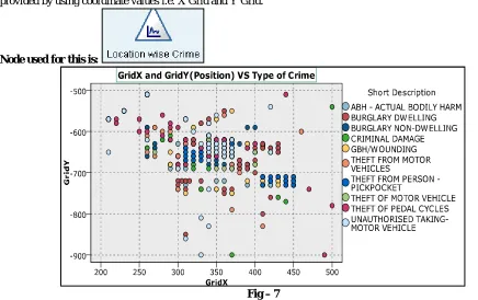
6. Below figure (Fig-7) represents the occurrence of various crimes location wise. In the data file location is provided by using coordinate values i.e. X Grid and Y Grid.
Node used for this is:
Fig – 7
Vol. 4, Issue 5, May 2015
Node used for this is:
Fig – 8
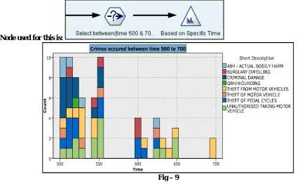
8. Below figure (Fig-9) represents the occurrence of various crimes based on the timing between 500 to 700. Here we have done slicing based on Fig-8 analysis. Here we have taken the help of “Select” Node to filter specific records.
Node used for this is:
Fig – 9
Vol. 4, Issue 5, May 2015
Node used for this is:
Fig - 10
10. Below figure (Fig-11) represents the various crimes which have occurred during month number 6 and on 5th Day.
Node used for this is:
Fig - 11
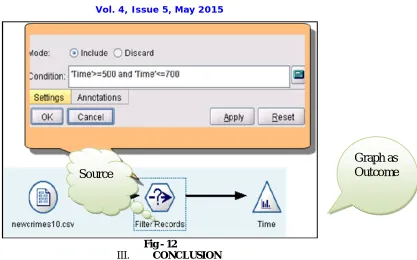
Vol. 4, Issue 5, May 2015
Fig - 12
III. CONCLUSION
As we have said at the beginning that, from a huge dataset, how quickly we can be able to find out information which can help us in doing better planning. This tool do have very good features to do various kind of analysis. Here we have taken only those nodes or functionality in to consideration, which was required for this case.
REFERENCES
1. Building the Data Warehouse William H. Inmon
2. The Data Warehouse Toolkit Ralph Kimball
3. www.spss.com/clementine
4. Data Mining Techniques by Arun k. Pujari