Bottleneck Effect on Evolutionary Rate in the Nearly Neutral Mutation Model

(1)

Bottleneck Effect on Evolutionary Rate

in

the Nearly Neutral Mutation Model

Hitoshi Araki

and Hidenori Tachida

Department of Biology, Faculty of Science, Kyushu University, Fukuoka, 812 Japan

Manuscript received December 2, 1996 Accepted for publication June 13, 1997

ABSTRACT

Variances of evolutionary rates among lineages in some proteins are larger than those expected from simple Poisson processes. This phenomenon is called overdispersion of the molecular clock. If population size Nis constant, the overdispersion is observed only in a limited range of 2Nu under the nearly neutral mutation model, where u represents the standard deviation of selection coefficients of new mutants. In this paper, we investigated effects of changing population size on the evolutionary rate by computer simulations assuming the nearly neutral mutation model. The size was changed cyclically between two numbers, N, and N2 (N, > N2), in the simulations. The overdispersion is observed if 2N2u is less than two and the state of reduced size (bottleneck state) continues for more than -0.1 / u generations, where u is the mutation rate. The overdispersion results mainly because the average fitnesses of only a portion of populations go down when the population size is reduced and only in these populations subsequent advantageous substitutions occur after the population size becomes large. Since the fitness reduction after the bottleneck is stochastic, acceleration of the evolutionary rate does not necessarily occur uni- formly among loci. From these results, we argue that the nearly neutral mutation model is a candidate mechanism to explain the overdispersed molecular clock.

T

HE mechanism of molecular evolution has been debated for a long time and we still do not have a clear-cut answer to this issue (see LEWONTIN 1974; KIMURA 1983; GILLESPIE 1991 )

. However, recent ad-

vances in molecular techniques enables us to test various hypotheses on the evolutionary mechanism by com- paring theoretical expectations of quantities with their estimates obtained from sequence data.

One such quantity is the evolutionary rate. Under the neutral theory of molecular evolution ( MMuRA 1968), evolutionary rates equal mutation rates. Thus, if the mutation rate is constant, the evolutionary rate becomes constant (molecular clock) and the substitution process is approximated by a Poisson process. There- fore, one way to test the neutrality of the substitution process with a supplementary condition of equal mutation rate among lineages is to examine whether it is Poisson or not ( OHTA and KIMURA 1971; LANGLEY and FITCH 1974). A useful parameter to characterize the substitution process is the dispersion index, I ( t ) , de- fined as (see, for example, TAKAHATA 1987)

where X ( t ) represents the number of substitutions in t generations and E and Var designate the expectation and variance operators, respectively. If X ( t ) is a Poisson process, the dispersion index I ( t ) is 1. GILLESPIE (1989) estimated I ( t ) using 20 mammalian proteins

Corresponding author: Hidenori Tachida, Department of Biology, Faculty of Science, Kyushu University, 33, Fukuoka, 812 Japan. E-mail: htachscbQmbox.nc.kyushu-u.ac.jp

analyzed by LI et al. (1987) and obtained estimates much larger than 1 (about

7-8)

.

Thus, the substitution process in this case is overdispersed. Since I ( t ) is one under the assumptions of the selective neutrality and constancy of mutation rates, it is worthwhile to investigate the behavior of I ( t ) in various other models (see TAKAHATA 1987, 1991; GILLESPIE 1991).

One such model worth investigating in this context is the nearly neutral mutation model proposed by OHTA (1972, 1992a) in which the substitution rate depends on the effective population size. Indeed, some of the recent data of mammals and Drosophila (e.g., OHTA 1993a,b; EASTEAL and COLLET 1994;

BALLARD

and KREITMAN 1994; NACHMAN et al. 1996) are indicative of nearly neutral evolution of nonsynonymous substitutions. Since population size is expected to change through time and among lineages, we expect fluctua- tion of substitution rates and larger dispersion indices if nearly neutral mutations contribute significantly to molecular evolution. However, effects of size change on evolutionary rate in the nearly neutral mutation model have not been quantitatively understood.

The main purpose of the present paper is to study effects of population bottlenecks (severe reductions of population size ) on evolutionary rate in the nearly neutral mutation model. TAKAHATA (1987) studied bottleneck effects on the dispersion index in a slightly deleterious mutation model and found that a very severe bottleneck with a fairly long duration is necessary to inflate the dispersion index. In the study, he used a mutation scheme called the shift model (OHTA 1977) in which the difference between the fitness of the mutated and

(2)

908 H. Araki and H. Tachida

original alleles was assumed to have a fixed distribution. OHTA and TACHIDA (1990) proposed the house-of- cards model of KINCMAN (1978) as a mutation model of protein evolution. In the house-of-cards model, the fitness of the mutant allele, not the difference between the mutated and original alleles as in the shift model, has a fixed distribution. This model was considered more appropriate as a mutation scheme for protein evolution since no limit is imposed on the fitness of protein in the shift model and this leads to, unrealisti- cally, infinite improvement or deterioration by succes- sive substitutions ( OHTA and TACHIDA 1990; OHTA 1992). Although there is no direct evidence to show that the house-of-cards model is appropriate for protein evolution, it is certainly worthwhile to theoretically investigate its property as a viable model. Here we adopt the house-of-cards model to characterize effects of mutation and investigate the dispersion index I ( t ) when population size cyclically fluctuates. Large dispersion indices are known to result under the house-of-cards model, though only in a small parameter range, even if the population size is kept constant ( GILLESPIE 1994; see also IWASA 1993). In the following, we first describe the model briefly. Then results of computer simulation are mentioned. Since we want to observe long term evolution when population size fluctuates, we use an approximate method in the simulation whose accuracy was checked by the exact Wright-Fisher type simulation. Finally, we develop an approximate formula to compute

I ( t ) and use this to obtain the time duration of bottlenecks necessary to make I ( t ) larger than one. We found that a fairly short duration of bottlenecks can inflate the dispersion index.

MODEL AND SIMULATION

Model: A haploid Wright-Fisher model is assumed in this paper. We assume that the size of the population is first Nl for tl generations and then shifted to N2 for

b2 generations ( Nl

>

N 2 ) . These two periods constitute one cycle and evolution in several cycles is investigated. Here, all of the four parameters, N, and tL’s, are constant. This constancy seems unrealistic because we expect these parameters to be randomly determined among lineages and through time in nature. However, we make this assumption to concentrate on the effect of population bottlenecks on the evolutionary rate elim- inating those from differences in Ni and ti and only a limited amount of simulation was carried out to see effects of stochasticity oft, . We adopt the house-of-cards model for mutation (KINGMAN 1978). Let u be the mutation rate. In this model, all new mutations result in new alleles (the infinite allele model of K”RA and CROW 1964) and the selection coefficient of a new mutant is drawn from a fixed probability distribution (see OHTA and TACHIDA 1990; TACHIDA 1991 ) . The mean and variance of the distribution are assumed to be zero

and D ‘ , respectively. Since 2 N p is an important param-

eter in the nearly neutral mutation model for character- izing its behavior, we designate it by a,.

Simulation: Since it takes much time to simulate the

Wright-Fisher model exactly by changing gene frequen- cies each generation (We call this the W-F simulation hereafter), we use an approximation that is expected to work when

Nu

is much smaller than one, where N

represents population size. This approximation is based on a Markovian jump process in which the fixation or loss of a mutant in the population occurs instantaneously. Consequently, the population is fixed with one allele at any moment and thus characterized by the selection coefficient of the fixed allele. We briefly describe this approximate method (see TACHIDA 1991 for more detail). We first determine the number, K ( t ) , of mutants that occurred in a duration t . I(( t ) is distributed as Poisson with a mean, Nut. We number mutants in the order of their occurrence times. Let h (

&,

S,) be the fixation probability of the kth mutant with selection coefficient Rk in the population fixed with an allele whose selection coefficient is

&.

In other words, Sk is the average selection coefficient of the population when the kth mutant occurred. The fixation probability was obtained by KIMURA (1962) and is expressed as

With this probability, the kth mutant is fixed and S,,,

=

&.

If the kth mutant is not fixed, then

Sk+]

=

&.

In our model, the population size is changed cyclically between Nl and N2 with duration tl and b , respectively. Therefore, in the implementation of the simulation, we determine K ( T ) and follow the change of Sk

for each period ( T = tl or and N = Nl or N 2 ) . The connection of two consecutive periods is made through equating the average selection coefficient of the population at the time junction. In the simulations, we first use the normal distribution as the probability distribution of mutant effects. The effect of the shape of the distribution will be examined by employing the uniform distribution later. The number, X ( t ) , of substitutions up to time t is expressed as

K ( 1 )

x ( t )

=

c

X ( h ( & , S k ) ) , ( 3 )

k= 1

where

x

( p )

is a random variable that returns one with probability p and zero with a probability 1 -

p . Then,

from the definition ( 1 ) of the dispersion index, I ( t ) can be estimated by replicating simulations. Note that

(3)

TABLE 1

Comparison of average number of substitutions and the dispersion index between

the approximate and W-F simulations

2(

t )

i(

t) a

2 N 1 ~ a 2 W-Fb Approx.' W-F' Approx."

0.1 2.0 5.50 5.40 1.650 5 0.100 1.618 2 0.097

0.2 20 4.03 4.21 0.393 t 0.017 0.405 +- 0.017

2.0 5.50 5.39 1.677 2 0.089 1.573 2 0.095

0.2 16.52 17.13 0.809 2 0.035 0.885 2 0.039

0.5 2.0 5.36 5.55 1.610 t 0.086 1.545 t 0.098

1

.o

2.0 5.15 5.57 1.778 2 0.087 1.576 t 0.099

2.0 2.0 4.97 5.77 1.917 +- 0.109 1.650 2 0.085

Other parameters are as follows: a1 = 200, utl = ut, = 10, UT = 30 (total generation length times mutation

"Values are +- SE, estimated by the jackknife method. 'Values computed from the W-F simulations.

'Values computed from the approximate simulations. rate), and r = 1000 (number of replications).

BULMER (1989) (see also GOLDMAN, 1994) and we do not consider this statistical problem in the following. The parameters that characterize the process are ai =

2N,a and ut, in this approximation ( i = 1, 2; see TA- CHIDA 1996). We tried several combinations of different values of these parameters. In all simulations, the initial selection coefficient is 0 and 1000 replications are made for each parameter set. In addition to the estimate of I ( t )

,

we also computed the variance of the estimate of I ( t ) using the jackknife method (see, for example, WEIR 1990, p. 137).

Accuracy of approximation: First, we checked the approximation method by carrying out the W-F simulation. The accuracy of this approximation was examined by TACHIDA ( 1991 ) when population size was constant and this approximation was found to work well for

2

Nu 4 1. Here, we examined only one and a half cycles (i.e., tl

+

4,

+

tl generations) because the W-F simulation takes much more time than the approximate method. Some of the results of the W-F simulations and the approximate simulations with the same parameter sets are shown in Table 1. The difference between the two simulations is expected to be large as 2N, u becomes large. But even for 2N1u = 0.5, fairly good agreements are found and for smaller 2N1u ( <0.2) , the approximate method works quite well. Thus, we can use this approximation if 2N,u is small.

Simulation result: The parameter ranges we studied are 0.02 I a2 I a 1 I 2000 and 0.01 5

ut,

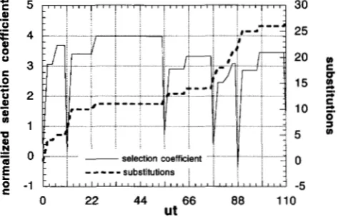
5 utl 5 10

in the approximate simulations. In all simulations, 10 cycles are observed. Figure 1 shows the fitness change and the accumulated number of substitutions in a typi- cal run of simulation. In this example, the length of a cycle, ut]

+

uk, is 11. Note that most changes of fitness and substitutions occur around multiples of 11 when population size is reduced and then recovered. One thousand replications of such runs are made for each parameter set and the columns with a header cyclic in

Table

2

shows estimates of the mean number of substitutions and dispersion index in the simulations when population size changes cyclically. To remove the effects of initial conditions, substitutions in the last seven cycles of bottleneck events were used to compute the values in the table. First note that the number,

x(

t )

,

of substitutions is a decreasing function of both

a1

and

a p . The equilibrium substitution rate was shown to be a decreasing function of population size when the size is constant (TACHIDA 1996) and our results indicate that this is a general characteristic of the house-of-cards model. For a = 2.0, I ( t ) is reported to be larger than one even when the population size is constant ( GILLES PIE 1994), and this is observed in our approximate simulation ( a 1 = a2 = 2.0). The dispersion index is larger than one also when bottlenecks are introduced ( a p 5

0 . 2 ) . However, in these cases, population bottlenecks rather reduce the dispersion index.

In contrast, a different pattern appears when a1 is

30

25

20

15

10

5

0

I

---substitutions i . .

'

~

c -5

0 22 44 66 88 110

ut

FIGURE 1.-Changes of the average selection coefficient and accumulated number of substitutions. Average selection coefficient normalized by D and accumulated number of s u b stitutions are plotted. Parameters are utl = 10, ut2 = 1, a1 =

(4)

910 H. Araki and H. Tachida

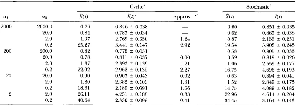
TABLE 2

Average number of substitutions and dispersion indices (normal distribution)

Cyclic" Stochastich

f f l f f P

2(

t )

i(

t ) Approx. T'

?(

t )

i(

t )

2000 2000.0 0.76 0.846 ? 0.038 - 0.60 0.851 ? 0.035

20.0 0.84 0.783 ? 0.034 - 0.62 0.865 t 0.038

2.0 1.07 2.769 ? 0.350 1.24 0.87 2.155 ? 0.231

0.2 25.27 3.441 t 0.147 2.92 19.54 5.903 ? 0.243

200 200.0 0.82 0.775 ? 0.031 - 0.58 0.805 ? 0.033

20.0 0.78 0.811 ? 0.037 0.00 0.59 0.819 +- 0.026

2.0 1.37 2.393 2 0.139 1.21 1.06 2.555 ? 0.177

0.2 22.02 2.962 ? 0.132 2.27 16.75 4.696 ? 0.193

20 20.0 0.90 0.903 ? 0.043 0.02 0.63 0.894 ? 0.041

2.0 1.80 2.382 ? 0.109 1.31 1.52 2.849 ? 0.173

0.2 18.61 2.189 ? 0.091 1.66 14.75 4.089 ? 0.182

2 2.0 26.11 4.251 ? 0.188 0.33 22.96 4.614 t 0.204

0.2 40.64 2.330 ? 0.099 0.41 34.45 3.164 ? 0.143

Other parameters are as follows: utl = 10, ut, = 1, uT = 110 (total generation length times mutation rate), and r = 1000

a Bottlenecks occur cyclically.

(number of replications). Approximate I w a s not computed when no shift occurs and consequently a = 0.

'Bottlenecks occurs stochastically.

'Values are -+ SE, estimated by the jackknife method. Values computed from the approximate formula.

larger. In these cases, I ( t ) is smaller than one when the population size is kept constant as observed by TACHIDA

( 1996). But when bottlenecks occur ( a g

<

a l ) , the dispersion index sometimes becomes larger than one. There seem to be optimal bottleneck sizes for large dispersion indices to be observed ( a 2 = 2.0 for a1 = 20.0 and a2 = 0.2 for a 1 = 200.0 and 2000). Thus, population bottlenecks inflate the dispersion index when selection is strong and the reduction of the population size is severe. In the next section, we consider why this happens and derive an approximate formula to compute I ( t )

.

Also reason for the existence of optimal bottleneck size for large I ( t ) will be considered there. To investigate the generality of the above finding, we employed the uniform distribution as the distribution of mutant effects and carried out simulation with the same parameter sets. Because the uniform distribution has very different tails from those of the normal distribution, different results were expected. Indeed, TA- CHIDA (1996) showed that substitutions continue to occur even when 2Na is 20 if the uniform distribution is used, while substitutions stop occurring after a while if we use the normal distribution. However, qualitatively similar results are obtained as shown in Table 3. The overdispersion is again observed for large Nl and small

N,, though the range of overdispersion is a little wider for the uniform distribution. Thus, large dispersion indices observed here when population size is changed seem to be general phenomena in the house-of-cards mutation model.

We also examined the effect of random occurrences of bottleneck events. We assumed that both utl and ut2 are exponentially distributed with the same means as

those o f the cyclic case and a1 and a2 are constant. The results are shown in the last two columns of Table 2 . If we introduce stochasticity, the dispersion index increases significantly when a 1 is large and a2 is small.

APPROXIMATE ANALYSIS

We consider a compound point process whose behavior mimics that of the Markovjump process investigated in the simulation. As shown in Figure 1, if a 1 is large, a burst of substitutions occur occasionally when the population size is reduced and then recovered ( ut =

11, 5 5 ,

77,

88 in this example )

.

We regard this episode of fitness reduction and recovery an event. Other than these, substitutions rarely occur for large a ] . In the approximation, we assume these multiple substitutions occur instantaneously in each event in some lineages. To accommodate stochastic bottleneck events, we assume that the number, M ( t ) , of events up to time t is a random variable and we designate its mean and variance by p M and

aL,

respectively. Also let be the number of substitutions in the ith event and its mean and variance are pLy and a:, respectively. We assume that M and Y,s are all mutually independent. Using a similar argument as that described in GILLESPIE (1991, p. 125),

Z(

t ) is computed to be

Z ( t ) =

#&/A;

+

( 4 ) For our problem of the deterministic bottleneck

PMP Y

model ( 0 % = O ) ,

a:

I ( t ) = - . ( 5 )

(5)

91 1

TABLE 3

Average number of substitutions and dispersion indices (uniform distribution)

a 2

i(

t )

I(

t ) Approx.

2000 2000.0

20.0 2.0 0.2 200 200.0

20.0 2.0 0.2

20 20.0

2.0 0.2

2 2.0

0.2

0.56 1.18 7.80 24.19 0.88 1.30 6.94 20.70 4.31 8.81 20.58 40.79 48.13

0.841 2 0.036 1.854 2 0.116 3.531 ? 0.170 2.438 t 0.104 1.007 ? 0.047 1.310 t 0.064 2.665 ? 0.111 2.289 +- 0.101 1.476 t 0.060 1.930 ? 0.085 1.759 ? 0.077 1.741 t 0.076 1.490 2 0.069

0.027 1.08 2.87 2.02 0.10 0.59 2.1 1 1.66 0.13 1.04 1.09 0.11 0.18

Other parameters are as follows: utl = 10, ub = 1, UT =

110 (total generation length times mutation rate), and T =

1000 (number of replications).

"Values are ? SE, estimated by the jackknife method. 'Values computed from the approximate formula.

Further simplification results if a bottleneck event in- duces a fitness reduction followed by recovery resulting in a substitutions with a probability

p

( the shift probability) or does not induce a fitness reduction resulting in 6 substitutions with a probability 1 -

p

( a

>

6 ) . Then

Using this expression, we can approximately compute

I(

t )

,

once we know a , 6, p . Unfortunately, it is difficult

to compute these parameters analytically. Thus, we need to estimate them from simulation and ( 6 ) does not seem useful. However, as shown below, the averages

of a and 6 are fairly constant for u& 5 1. Furthermore,

the shift probability

p

is computed given ut2 and the expected average selection coefficient, so, of the population just before the bottleneck event. Thus, ( 6 ) has some predictive power for u& 5 1 even though a , 6, so

are estimated from simulation.

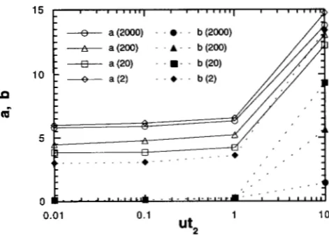
First, we examine the dependency of a and 6 on u& estimating them from the simulation (Figure 2 ) . In each bottleneck event (reduction and recovery of population size), if the fitness at the beginning of a bottleneck period is higher than that at the end of it, we regard that the shift occurred and the number of substitutions in the cycle (bottleneck and recovery) is counted as a . Otherwise, the number of substitutions is counted as 6. We averaged a and 6 obtained in this way in the last seven cycles as in the previous section. As shown in the figure, a is almost independent of ut2 for uL2 5 1.0. Probably most of a substitutions are non-

neutral occurring just after the size changes and thus

a becomes fairly constant as ut2 changes in this range. Next, we compute the shift probability,

p (

uh) , as

10

5

0

"8- a(2000) - - 0 - - b(2000)

+

a (200) - - A - - b (200)

"0- a (20) - - - - b (20)

+

a(2) - - e - . b(2)

0.01 0.1 1

ut2

10

FIGURE 2.-Dependency of a and b on the length of bottleneck. a ( x ) and b (x) represent a and b , respectively, for a ,

= x. The length of bottleneck is standardized by the mutation

rate. Other parameters are a2 = 0.2 and utl = 10.

a function of uh. For the shift to occur, at least one deleterious substitution has to occur after the population size reduction. Although precisely one-half of sub- stitutions are deleterious in the equilibrium state under the house-of-cards model ( GILLESPIE 1994), the first substitution after the reduction of population size is most likely a deleterious one, since the fixation probability of deleterious mutations increases very much after the reduction. Thus, from

(2),

the transition rate, A, for a shift may be approximately expressed as

where f( s ) is the standardized distribution of mutation effects and S, is the standardized fitness of the population just before the bottleneck. As a rough estimate of

S,

, we use its average, so, estimated from simulation to compute A and the shift probability

p

( ub) is expressed as

Estimates of s,,, a and 6 are shown in Table 4. Using these estimates, ( 8 ) and ( 6 ) , we can approximately compute I( t ) and the approximate values thus computed are shown in Tables 2 and 3. For a 1 2 20 and

a 2 5 0.2, the approximate values are similar to those

obtained by the simulation although the former always underestimate the latter (see also Figure 3 ) . The reason for the underestimation may be due to neglecting the variance of the number of substitutions, a , when the shift occurs. Indeed, if we put the estimated variance of a into ( 5 ) , we obtain better agreements (data not shown )

.

(6)

912 H. Araki and H. Tachida

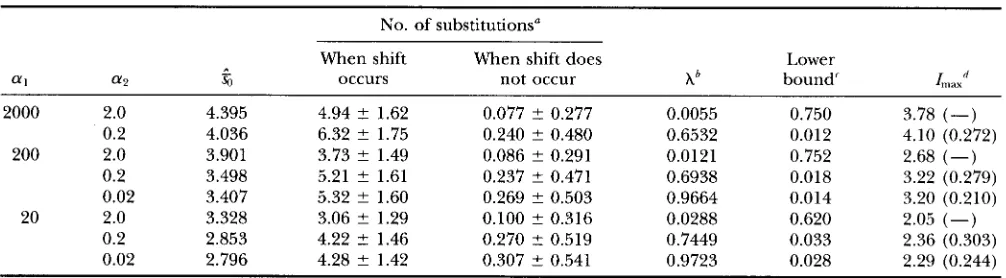
TABLE 4

Estimates of SO, a, b from simulation, approximate values of the lower bound of ut2 that produces overdispersion and the maximum dispersion index

No. of substitutions"

When shift When shift does Lower

f f l f f 2 %J occurs not occur Ab bound'

Lax''

2000 2.0 4.395 4.94 ? 1.62 0.077 ? 0.277 0.0055 0.750 3.78 (-)

200 2.0 3.901 3.73 ? 1.49 0.086 ? 0.291 0.0121 0.752 _2.68(-)

0.2 4.036 6.32 ? 1.75 0.240 ? 0.480 0.6532 0.012 4.10 (0.272)

0.2 3.498 5.21 ? 1.61 0.237 ? 0.471 0.6938 0.018 3.22 (0.279)

0.02 3.407 5.32 ? 1.60 0.269 ? 0.503 0.9664 0.014 _{3.20 (0.210)}

0.2 2.853 4.22 2 1.46 0.270 ? 0.519 0.7449 0.033 2.36 (0.303)

0.02 2.796 4.28 ? 1.42 0.307 ? 0.541 0.9723 0.028 2.29 (0.244)

20 2.0 3.328 3.06 ? 1.29 0.100 ? 0.316 0.0288 0.620 2.05 (-)

Parameters so, a, b are estimated from simulation with utl = 10, ut, = 1, UT = 110 and r = 1000 (number of replications). "Values are ? SD.

* Rate of a shift [see

(7)].

'The approximate lower bound of ut when Z( ut2) becomes larger than one.

dApproximate values of the maximum, I,,,, and ~h~~~ (in parentheses) that produces the maximum Z when ut, is changed. -, if is more than one, it was not computed (see text)

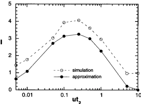
approximate values. From the figure, we can see that the approximation captures the behavior of I as ut2 changes fairly well for ut2

<

1 although the approximation mostly underestimates the true values as pointed out before. The qualitative agreement between the observed and approximate values suggests that the approximate treatment of the process essentially captures the mechanism to produce large I ( t )

.

In the derivation of ( 6 ) , we assumed that a burst of substitutions occur randomly when an event occurs in each lineage. Thus, if bottlenecks occur in the nearly neutral mutation model, multiple substitutions occur in some lineages while very few substitutions occur in other lineages and this is responsible for the overdispersion observed when

a 1 is large and a2 is small.

The magnitude of the dispersion index depends on the proportion of populations undergoing shift. If no population undergoes shift or all populations undergo shift, numbers of substitutions would not differ much among populations and the index will be small. Thus, an optimal proportion of shift is expected to exist for a large dispersion index to be observed. We can estimate the lower bound of

uh

for Z to be larger than one and the

uh

that maximizes I when N l , tl

,

N2 are kept constant from ( 6 ) . The upper bound of ut2 cannot be estimated because it is usually larger than one, and a and b are no longer constant as ut2 changes. The pre- dicted lower bound and maxima are computed from estimates of a, b , and shown in Table 4. As shown in the table and figure, I is larger than one even when ut2 is 0.02 and fairly large I is observed for ut2 around 0.1. Finally, we can assess the effect of random occurrences of bottleneck events from ( 4 ) . To derive ( 6 ) , we assumed that bottleneck occurs regularly and thus

U L

= 0. If

U L

>

0, I ( t ) is inflated because

crL

appears

only in the numerator of I ( t ) in ( 4) and this is indeed observed in our simulation (see Table 2 )

.

DISCUSSION

In the present paper, we investigated the effect of changing population size on the substitution rate in the nearly neutral mutation model. We found from the simulation that if the population size fluctuates between large ( N l ) and small ( N 2 ) with conditions, a , s 20 and

a2 5 2.0, the dispersion index becomes larger than

one. From the approximate analysis, the large dispersion indices are considered to result from multiple substitutions that occur only in a portion of populations when the reduction and recovery of population size take place. The approximate analysis shows that bottleneck events with fairly short periods (ut2

-

0.1 or less) can inflate the dispersion index.

(7)

I

3

2

1

0

\

-

-e

- - simulation

"-4- approximation

' 1

b -

0.01 0.1 1

ut*

10

FIGURE 3.-Estimates of Zfrom simulation and approximation. Z is plotted as a function of u k . Other parameters are

a , = 200, a2 = 0.2 and utl = 10.

because not many degrees of freedom are left for test- ing. In Goldman's analysis, only four and three species were used for a-hemoglobin and cytochrome oxidase

2,

respectively. What GILLESPIE (1989) did is to remove lineage effect by the average nonsynonymous substitutions of all ( 20) protein genes analyzed. Thus, a large estimate of Z by GILLESPIE ( 1989) cannot be ascribed to the inclusion of lineage effects. Also the inflation of the estimate of Zdue to covariance terms pointed out by BULMER (1989) is not much because corrections for multiple hits is small in the estimation of nonsynonymous substitutions (see p. 120 of GILLESPIE 1991 )

.

Re- cently OHTA ( 1995) analyzed 49 mammalian protein data and obtained an estimate of 5.6 when the average of nonsynonymous rate is used to weight the branches. Although OHTA'S estimate is a bit smaller than that of GILLESPIE, the dispersion index in mammals seems to be five or larger. In our simulation, the dispersion index as large as five or six was observed when the population size is changed stochastically. Thus, the nearly neutral mutation model with changes of population size may be sufficient to account for the estimate of the dispersion index in mammals.

To save computation time, we used a Markovian jump process to approximate the process. If we consider the points where substitutions occur, this is a continuous time-dependent version of the semi-Markov process studied by TAKAHATA (1991; see also IWASA 1993). In the subsequent analysis, we further approximated the process by a compound point process and suggested that random occurrences of multiple substitutions are responsible for the overdispersion. Since multiple substitutions are known to be a source of overdispersion (TAKAHATA 1987), it is not surprising to find overdispersion in the present case from the standpoint of the theory of point processes. However, point processes are descriptive models of substitution processes. There- fore, substitution processes of many different evolution-

ary models can be described by the same point processes. For example, TAKAHATA ( 1987) lists intramolec- ular interactions and some mutational changes creating more than one nucleotide change as causes of multiple substitutions at a time. What we showed here is that the house-of-cards mutation model as a mechanistic model of molecular evolution gives rise to overdispersion under certain conditions when population size is changed. Although this scenario was verbally stated by OHTA

( 1995) and GILLESPIE ( 1995) , we quantified their pre- diction and examined the process by approximating it with a compound process.

TAKAHATA (1987) studied effects of the reduction of population size on the evolutionary rate of slightly deleterious mutations. He found that very severe bottlenecks whose mode differs among lineages and a very high mutation rate are necessary for the contribution from deleterious mutations to inflate the dispersion index. His result seems to contradict what we obtained here because fairly short durations of bottlenecks can inflate the dispersion index above one in our simulation. The reason for the discrepancy lies in the different mutation schemes adopted in the two studies. TAKA- HATA (1987) used the shift model (see OHTA and TACHIDA 1990) as a mutation scheme and all mutations are deleterious. Thus, the substitution rate never ex- ceeds the mutation rate. On the other hand, we used the house-of-cards model and multiple substitutions in- cluding deleterious and advantageous ones occur in a short period. Thus, only a short duration of the reduction of population size ( utz, = -0.1 or less) is necessary to inflate the dispersion index above one. Moreover, since multiple substitutions occur randomly among lineages, the mode of bottlenecks needs not be different among lineage. So the condition for larger dispersion indices is less stringent in the house-of-cards model than in the shift model.

One of the questions in assessing the validity of the present model to explain the overdispersion is whether bottlenecks of lengths considered here (ut2 = -0.1 or even less) are plausible or not. Since estimated values of mutation rate are in the order of or so per year in the nuclear genes (MUKAI and COCKERHAM 1977; NEEL et al. 1986), the length of the bottleneck must be longer than

lo5

years or so. One candidate mechanism that causes bottlenecks of this scale is the 100-kyr glacial- interglacial cycle observed in the past 800 kyr (see GATES 1993). For many species living in warmer areas, population sizes were expected to be reduced in glacial periods. For mitochondrial genes that have higher mutation rates, even shorter bottlenecks may inflate the dispersion index.

(8)

914 H. Araki and H. Tachida

be considered as an evidence against the hypothesis that the acceleration is due to slightly deleterious mutations fixed by bottleneck events. However, as shown in the present paper, even if the distribution of mutant effect is the same, a burst of substitutions occur in some genes but very few substitutions occur in other genes in the same organism when bottlenecks occur. Thus, such an argument cannot be used to reject the nearly neutral mutation theory.

We thank M. IIZUKA and two anonymous referees for valuable com- ments on the manuscript. This research was partially supported by a grant-in-aid to H.T. from the Ministry of Education, Science and Culture of Japan and Sumitomo Foundation.

LITERATURE CITED

BAI-LARD, J. W. O., and M. KREITMAN, 1994 Unraveling selection in the mitochodrial genome of Drosophila. Genetics 138: 757-772. BULMER, M., 1989 Estimating the variability of substitution rates.

Genetics 123: 615-619.

EASTEAL, S., and C. COLLET, 1994 Consistent variation in amino-acid substitution rate, despite uniformity of mutation rate: protein evolution in mammals is not neutral. Mol. Biol. Evol. 11: 643- 647.

GATES, D. M., 1993 Climate Change and Its Biolvpal Consequences. Sinauer Associates, Sunderland,

MA.

GILLESPIE, J. H., 1989 Lineage effects and the index of dispersion of molecular evolution. Mol. Biol. Evol. 6: 636-647.

GILLESPIE, J. H., 1991 The Causes of Molecular Evolution Oxford Uni- versity Press, New York.

GILIXSPIE, J. H., 1994 Substitution processes in molecular evolution.

111. deleterious alleles. Genetics 138: 943-952.

GILLESPIE, J. H., 1995 On Ohta’s hypothesis: most amino acid substitutions are deleterious. J. Mol. Evol. 4 0 64-69.

GOLDMAN, N., 1994 Variance to mean ratio, R ( t ) , for Poisson processes on phylogenetic trees. Mol. Phylogenet. Evol. 3: 230-239. IWASA, Y . , 1993 Overdispersed molecular evolution in constant envi-

ronments. J. Theoret. Biol. 164: 373-393.

KIMURA, I C , 1962 On the probability of fixation of mutant genes in a population. Genetics 47: 713-719.

KIMURA, M., 1968 Evolutionary rate at the molecular level. Nature

217: 624-626.

KIMURA, M., 1983 The Neutral T h e q of Molecular Evolution. Cam-

bridge University Press, Cambridge.

KIMURA, M., and J. F. CROW, 1964 The number of alleles that can he maintained in a finite population. Genetics 4 9 725-738.

KINGMAN, J. F. C., 1978 A simple model for the balance between selection and mutation. J. Appl. Probab. 15: 1-12.

LANGLEY, C. H., and C. H. FITCH, 1974 An estimation of the constancy of the rate of molecular evolution. J. Mol. Evol. 3: 161-

177.

LEWONTIN, R. C., 1974 The Genetic Basis of Evolutionaly Change. Cc-

lumbia University Press, New York.

LI, W-H., M. TmIwuRAand P. M. SHARP, 1987 An evaluation of the molecular clock hypothesis using mammalian DNA sequences. J.

MUM, T., and C. C. C O C K E ~ , 1977 Spontaneous mutation rates at enzyme loci in Drosophila melanogaster. Proc. Natl. Acad. Sci. USA 74: 2514-2517.

NACHMAN, M. W., W. M. BROWN, M. STONEKING and C. F. AQUADRO, 1996 Nonneutral mitochondrial DNA variation in humans and chimpanzees. Genetics 1 4 2 953-963.

NEEL, J. V., C. SATOH, K. GORIKI, M. FUJITA, N. TAKAHASHI et al., 1986 The rate with which spontaneous mutation alters the electropho- retic mobility of polypeptides. Proc. Natl. Acad. Sci. USA 83:

OHTA, T., 1972 Population size and rate of evolution. J. Mol. Evol.

OHTA, T., 1973 Slightly deleterious mutant substitutions in evolution. Nature 246: 96-98.

OHTA, T., 1977 Extension to the neutral mutation random drift hypothesis, pp. 148- 167 in Molecular Evolution and Polymmphzsm,

edited by M. KIMURA. National Institute of Genetics, Mishima, Japan.

OHTA, T., 1992 The nearly neutral theory of molecular evolution. Annu. Rev. Syst. Ecol. 23: 263-286.

OHTA, T., 1993a Amino acid substitution at the Adh locus of Drosoph- ila is facilitated by small population size. Proc. Natl. Acad. Sci.

OHTA, T., 199313 An examination of the generation-time effect on molecular evolution. Proc. Natl. Acad. Sci. USA 90: 10676-

10680.

OHTA, T., 1995 Synonymous and nonsynonymous substitutions in mammalian genes and the nearly neutral theory. J. Mol. Evol.

40: 56-63.

OHTA, T., and M. KIMURA, 1971 On the constancy of the evolutionary rate of cistrons. J. Mol. Evol. 1: 18-25.

OHTA, T., and H. TACHIDA, 1990 Theoretical study of near neutrality. I. Heterozygosity and rate of mutant substitution. Genetics

TACHIDA, H., 1991 A study on a nearly neutral mutation model in

TACHIDA, H., 1996 Effects of the shape of distribution of mutant

TAKAHATA, N., 1987 On the overdispersed molecular clock. Genet-

TAKAHATA, N., 1991 Statistical models of the overdispersed molecu-

WEIR, B. S., 1990 Genetic Data Analysis. Sinauer, Sunderland, MA. Mol. Evol. 25: 330-342.

389-393.

1: 305-314.

USA 90: 4548-4551.

126 219-229.

finite populations. Genetics 128: 183-192.

effect in nearly neutral mutation models. J. Genet. 75: 33-48.

ics 116: 169-179.

lar clock. Theoret. Popul. Biol. 3 9 329-344.