20th International Conference on Structural Mechanics in Reactor Technology (SMiRT 20) Espoo, Finland, August 9-14, 2009 SMiRT 20-Division III, Paper 2489
Systematic Errors in the Numeric Analyses of Computer Programs Employed
for the Determination of the Flexible Structure Seismic Response
Viorel Serban, Marian Androne
SITON - Subsidiary of Technology and Engineering for Nuclear Projects, Bucharest, Romania, [email protected]
Keywords: Initial velocity, long periodical component, response spectra, accelerogram, seismogram.
1
ABSTRACT
At present the determination of the building seismic response is done by finite element computer models, by in-time or frequency dynamic response analyses of the building.
For the in-time analyses, the computation is just the solving of a differential equation system of 2nd degree in the relative displacement variables, for which the initial conditions (displacement and velocity) need to be specified. All the current computer programs known by the authors are considering null values for both relative displacement and velocity as initial conditions. In the most cases, the initial relative velocity cannot be zero and considering it null is introducing errors in the determination of the seismic response. These errors are important when speaking about flexible buildings such as tall buildings, seismically isolated buildings or buildings where plastic hinges are accepted.
The paper is an evaluation of the calculation errors resulted from the computer programs employed today (the examples are based on the results obtained with a commercial computer program, called “CP” in the paper) in the calculations for structures and it also includes solutions to eliminate such errors. Also, the errors occurring in the determination of the relative displacement response spectra for earthquakes with time-history acceleration records are performed.
2
INTRODUCTION
The analysis on the building seismic behaviour is made by solving a differential equation system whose size depends on the mesh of finite elements used for modelling the structures. In order to relieve the systematic calculation errors in the current computer programs for structures and their quantification as to the theoretical solutions, the analyses are conducted for a simple system with one degree of liberty, SDOF. With systems of several degrees of freedom, the errors are similar. The analyses are aimed to determine the in-time variation of SDOF response (relative displacement, absolute displacement and acceleration), subjected to a harmonic excitation such as a seismogram and accelerogram.
3
EVALUATION OF ERRORS OF THE REPONSE IN DISPLACEMENTS FOR AN
OSCILLATING SYSTEM
3.1 Errors resulting from the initial velocity
In the conducted analysis, the SDOF model – which may model a building of mass, m, damping, c, and stiffness k, is subjected to a ground oscillating movement, marked by u(t), which is represented by a harmonic movement of Uo amplitude and Ts period, of the following form:
T
U
S t t t
u( )= 0sin", " = 2
!
(1)( ) ( ) ( )
t cx t kxt mu( )
t xm&& + & + =! &&s (2a)
( ) ( ) ( )
t cyt kyt ku( )
t cu( )
t ym&& + & + = s + &s (2b)
For eq. (2a) some computer programs employ (3a) as initial conditions (Ifrim, 1984, Cornea et al., 1987). For (2b), which has the total displacement as unknown variable, the initial conditions must be (3b):
( )
t
=
0
x
,x
&
( )
t
=
0
(3a)( )
t
=
0
y
,y
&
( )
t
=
0
(3b)From mathematical point of view, the conditions (3a) and (3b) are not equivalent and that will lead to calculation errors for the displacement variable (and generally, in the cinematic response of the system). Conditions (3b) which are assumed for the total displacement are evidently correct, namely:
( ) ( )
0
=
x
0
+
u
(
0
)
=
x
( )
0
+
0
=
0
y
, and y&( ) ( )
0 =x& 0 +V0 =0 . Starting from that situation, the initial conditions in the relative displacement variable need to be:( )
t
=
0
x
,x&( )
t =!V0 (3a’)(where V0 is the ground initial velocity) instead of the ones in (3a).
Fig. 3.1 shows the relative displacement of the SDOF system and the displacement excitation of 10cm amplitude and 1s period. The system relative displacement is obtained with eq. (2a) with initial conditions (3a) on systems with the vibration period (T = 10s) much greater than the excitation period (Ts = 1s), while
Fig. 3.2 illustrates the same results obtained with eq. (2b) and initial conditions (3b). The obtained results are very different as an effect of the incorrect initial conditions (3a).
Figure 3.1. Relative displacement of the system, using eq. (2a) and (3a) Input: time-history acceleration obtained from eq. (1) by derivation,
As(t) = 4sinΩt (m/s2).
Figure 3.2. Relative and total displacement of the system and the ground displacement, using eq. (2b) and (3b). Input: seismogram Us(t) = 0.1sinΩt (m).
Figure 3.3 illustrates the ground displacement obtained with “CP” computer program, considering the time-history acceleration As(t) = 4sinΩt (m/s
2
) as input. The exaggerated increase of the ground displacement at values of 2.55 m obtained from the two-times integration of the time-history acceleration is due to the fact that the program does not know the initial velocity which is considered zero in the analyses. Analyzing the diagrams, it results that in case of eq. (2a) and initial conditions (3a) the solution supplied by the computer program, is wrong. Evidently it is expected that for an eigen period of 10s, the system actually remains motionless, the total displacement being about zero and the relative displacement being equal and contrary as sign with the ground displacement (as presented in fig. 3.2).
Variatia in timp a deplasarii relative si a deplasarii terenului.
-1 -0.8 -0.6 -0.4 -0.2 0 0.2 0.4 0.6 0.8 1
0 5 10 15 20
Tim p, [s ]
D
e
p
la
s
a
re
,
[m
]
Figure 3.3. Ground displacement (measured in meters) obtained with “CP” computer program. Input: accelerogram As(t) = 4sinΩt (m/s2).
Figure 3.4. Relative and total displacement of the system and the ground movement, using eq. (2a) (3a’). Input: accelerogram As(t)=4sinΩt (m/s2).
From the analytical point of view, (Ifrim, 1984), such a thing implies the addition of a term proportional with the initial ground velocity, V0, and SDOF period, T, to the SDOF equation solution, x(t),
initially calculated with conditions (3a):
t
e
V
x
x
=
+
! " t#
!#
$#
sin
~
0(4)
a correction which becomes significant for long periods (flexible systems). This additional term is part of an analytical general solution which vanishes once the null initial velocity is considered. Therefore, for rigid and half-rigid systems the error generated by the initial conditions (3a) is having a small weight in the oscillating systems response, while for flexible systems, the error generated by the initial conditions (3a) has a great weight in the seismic response of buildings.
3.2 Errors generated by long harmonic periods of initial accelerograms
One should also consider the fact that the response in the displacements of an oscillating system in the long period range is strongly amplified by the presence of long period components in the excitation, though they may not be clearly found in the response in accelerations.
Let’s consider an accelerogram with two periodic components of equal amplitude. The absolute accelerations response spectrum has very close amplitudes, where the difference is given by the crossed contributions of the two components (fig. 3.5). In case of the relative displacement response spectrum the long period components are much amplified, proportionally with the vibration period (fig. 3.6), the crossed contributions of the two components being very small. The big difference between the amplitudes in the displacement response spectrum occurs when the two components are much spanned from each other.
Figure 3.5. Response spectrum of the absolute acceleration.
Figure 3.6. Response spectrum of relative displacements.
contributions of the other components, which generally are very small, mainly for distanced periods)
becomes: 2 2 2
8
2
ii
i i
i
T
A
A
X
=
!
"
=
#
$
#
which shows that the long period components lead to large amplitudes in the displacement response spectrum, even if that amplitude of the time-history component Ai is verysmall. Thus, the in-excess increases of the relative displacement amplitudes in the response spectra are due to two effects, namely: the phenomenon of real amplification of some long periods harmonic components (real or false in time series) in the seismic movement and the non-null initial velocity which is not considered in the calculation of the response spectra. Figure 3.6 shows that starting with T = 3s, the relative displacement response spectrum is affected by the effect of the initial velocity consideration. This example evidences the cumulated result of the two effects: the consideration of the null initial velocity and the amplification of the high period components.
3.3 Analysis of possible errors in recorded accelerograms
In order to outline the influence of the initial velocity and of the long period amplification on the response in the relative displacement for a real time-history, herein below it is a presentation of the results of the analyses conducted with real recorded time-histories, namely, for the earthquake “1952 KERN COUNTY”, figs. 3.7-3.8 and “1994 NORTHRIDGE EARTHQUAKE”, figs. 3.9-3.10.
The analyses consist in the comparative presentation on the same graph of the in-time variation of the relative displacements (figs. 3.7, 3.9), as follows: the calculation of the relative displacements by the direct application of the seismogram and the calculation of the relative displacements by using the accelerogram with the initial velocity estimated by Fourier method, the initial velocity given by the velocity time-history and using its zero value.
Figure 3.7. The “1952 KERN COUNTY”
earthquake. The relative displacement. Vibration period T = 100s. For v0 = 0 the maximum relative
displacement, Dmax = 365mm.
Figure 3.8. The “1952 KERN COUNTY”
earthquake. The relative displacement response spectrum.
Figure 3.9. The “1994 NORTHRIDGE
EARTHQUAKE”. The relative displacement. Vibration period T = 100s. For v0 = 0 the maximum
relative displacement, Dmax = 200mm.
Figure 3.10. The “1994 NORTHRIDGE
EARTHQUAKE”. The relative displacement response spectrum. For v0 = 0 the maximum
relative displacement, Dmax = 200mm.
Using Accelerogram as input (eq. 2a), with initial velocity from
Fourier Method Using Accelerogram as input
(eq. 2a), with initial velocity from Velocity Time-History
Using Accelerogram as input (eq. 2a), setting zero
for initial velocity Using Seismogram as input
The case of “1952 KERN COUNTY” earthquake. For T = 100s the maximum relative displacement obtained with “CP” computer program is Dmax= 374 mm, a value close to the value calculated independently
(fig 3.7). The comparison confirms that “CP” computer program is using the null initial velocity for the system response. If different initial velocities estimated by various methods (fig. 3.7) were used, small responses would be obtained: 136mm with Fourier method or 86mm (employing the initial velocity from velocity time-history). Directly applying the seismogram, one may obtain the maximum relative displacement Dmax= 68mm, identical with the ground maximum displacement (from seismogram) which is
Umax= 68mm.
The case of the “1994 NORTHRIDGE EARTHQUAKE”. For all the periods up to 100s the results are similar for all the applied methods, except the curve for which the seismogram and the initial velocity from the velocity time-history have been used. Even for T = 100s the maximum relative displacement obtained with SAP29000 is Dmax= 200mm (fig. 3.10), a value equal to the value in the independent calculation (fig.
3.9) for the methods: Fourier to estimate the initial velocity and the null initial velocity imposed. In case of using the seismogram, Dmax= 152mm. The comparison confirms that the initial velocity associated to the real
earthquake is very close to zero (V0=1 mm/s calculated by Fourier method), case in which the correction
term is negligible.
4
EVALUATION OF THE ERRORS IN THE RESPONSE SPECTRUM OF
DISPLACEMENTS
Considering the definition of the relative displacement response spectrum, such displacements need to fall-in some limit requirements which are also a measure of their determination, for example:
- the spectra need to have about zero value at very small periods;
- the spectral relative displacement need to be practically equal with the maximum ground displacement for very long periods;
- considering that the seismic movement contains several spectral components, it results that the response spectrum of the displacements shall be amplified in the long period range, with important amplitudes even for the acceleration time-history components of very low amplitude;
- the periods from which the response spectrum of the displacements starts to get asymptotically limited, depend on the frequency-content of the accelerogram. In case of the accelerogram having long period spectral components (such components may be introduced by the recording instrument or its location), the area of asymptotic limitation will start after these spectral components.
If several response spectra of displacements during important earthquakes published in literature are analyzed (Kelly, 2001), one may find that most of them do not satisfy the minimum requirements in point of correctness (fig. 4.1 and similar), namely: (i) the displacements response spectra are actually increasing uniformly in the range of long periods without evidencing the possible resonance zone of the seismic movement, and, (ii) in the range of long periods (over 2-3s in some cases, or 5-10s in other cases) the displacements are not asymptotically limited to the maximum ground displacement. Generally, they are continuously increasing, while for the response spectra of displacements in fig. 4.2 (and similar) they have a shape that meets the principles of physics.
Figure 4.1. Response spectrum of accelerations and displacements in horizontal plane for “1952 KERN COUNTY” earthquake.
Instead, for the absolute accelerations response spectra of analyzed earthquakes, the general requirements for correctness are fully satisfied. The reasons for the errors in the calculations of the relative displacement response spectra are the incorrect initial conditions specified. For response spectra whose shape and value are approximately meeting the general correctness requirements, it is likely that the ground velocity at moment t = 0 be V0
!
0, which makes that the additional term brings no contribution (fig. 4.2).5
SDOF ANALYSIS FOR THE 3s EIGEN PERIODS FOR A HARMONIC GROUND
MOTION
The purpose of the analysis is to estimate the system response and the associated errors for flexible systems of usual periods or seismically isolated systems.
Assume a sinusoidal seismogram (displacement time-history) of the period Ts= 1s that is to be used in
eq. (2b). One calculates the acceleration time-history corresponding to the seismogram that is to be used in eq. (2a) in two hypotheses: with zero and non-zero initial relative velocity. The results obtained by the use of the accelerogram in the two hypotheses shall be compared with the results obtained by the directly use of the seismogram and those supplied by the “CP” computer program. The seismogram is compatible with the accelerogram in point of amplitude and vibration period.
The calculations are done for an eigen vibration period T= 3s, value which is typical for high buildings or seismically isolated buildings. The numeric results presented in the following figures, consist in: Disp0 – ground displacement; Rel_Disp – relative displacement and Abs_Disp - absolute displacement.
Figure 5.2 Input: Seismogram Us(t)=0.05sinΩt.
Maximum relative displacement = 7.3cm. Maximum absolute displacement = 2.4cm.
Figure 5.4. Input: Accelerogram As(t)=2sinΩt.
Maximum relative displacement = 7.4cm. Maximum absolute displacement = 2.4cm. V0≠ 0.
Figure 5.6. Input: Accelerogram As(t)=2sinΩt.
Maximum relative displacement = 21.5cm. Maximum absolute displacement = 16.5cm. V0 = 0.
Figure 5.8. Relative Displacement Response Spectra. Results performed by “CP” computer program. Input: Accelerogram As(t) = 2sin Ωt.
Figure 5.9. Relative displacement performed with “CP” computer program and with independent numerical method and V0 = 0. Input: Accelerogram As(t) = 2sin Ωt (m/s2); Maximum relative
displacement, X = 21.5 cm (“CP” computer program results) and X = 21.5 cm (numeric calculation).
Remark 1. The “CP” computer program is calculating the ground displacement by double integration, for the us(0)=0 and u&s(0)=0conditions which are incorrect. Since the ground acceleration:
t A
t
u&&s( )= 0sin! ; A0 =2m/s2, then the analytic calculation of the ground movement becomes:
t A t A t
us !
! " # !
= sin )
( 0 02 ; T s
s =1 ; ⇒ us(40s)=12.73m, that is a value identical with the value given by
“CP” computer program, a fact that confirms its calculation procedure and its incorrectness. The analytical calculation was conducted by the double integration of the time-history considering null initial conditions for displacement and relative velocity. As a conclusion, for the calculation of the total displacement of a system “CP” computer program is calculating separately the ground displacement by the double numeric integration of the acceleration, without controlling the constants of integration which insert a linear term in time. Such a value is added to the value of the relative displacement which in its turn, is evaluated incorrectly, for the reasons presented above. Fortunately, the large error calculations of the total displacements do not introduce significant errors in the calculation of forces, moments and stresses because these are determined as gradient of the relative displacements along the calculated element.
Remark 2. It is found that for any SDOF eigen periods (analyzed being T=2s, 3s, T=4s in Serban et al., 2007, and 10s), the in-time variation of the relative displacements calculated by “CP” computer program and numerically calculated for a null initial velocity are identical. Such a fact is leading to the conclusion that “CP” computer program is employing null initial conditions for displacement and velocity in the determination of the relative displacements (generally the system response), conditions that are not correct. The initial ground displacement must be zero because the ground was at rest before the earthquake, meaning that the SDOF relative displacement becomes x(0) = 0, which is a correct initial condition. The ground initial velocity is not mandatorily zero (neither in this case, nor generally). It results,
0 ) 0 ( )
0 ( ) 0 ( ) 0
( = y "us ="us !
x& & & & , which mandatorily imposes that the initial relative velocity of SDOF be
equal with the ground initial velocity of changed sign. From the analytical point of view, this thing implies
the keeping of the term
u
!e
" t#
!t
#
$#
sin
0&
to the general analytical solution of SDOF equation, that is
computer code (which in calculations, consider null initial conditions for the initial velocity) are very much shifted from the real value, specially for flexible systems. This is the case of the response spectra which are increasing as the increase of the SDOF period (fig. 4.1)
Remark 3. Suppose the case when the seismic design codes (Romanian code P100/2006, European standards and others) base their seismic isolation procedure on the results supplied by accepted computer programs in which the response spectra are increasing with the increase of the period (which are erroneous, like the case in fig. 4.1 and similar). Then it is expected that the procedure and the sizing method in the design codes are not correct and lead to wrong design values. The computation error highlighted in this paper is affecting the sizing of flexible buildings such as the reinforced concrete framework buildings, seismic isolated buildings and quite high buildings where plastic hinges are accepted.
Remark 4. To correct the computer programs in view of eliminating or reducing the computation errors it is possible to apply the following alternatives:
1. The further use of the existing numeric computation procedures on basis of the generated/real/design accelerograms (eq. 2a) but the using of the initial conditions:x0 =0 andx&0 =!V0, where V0 – is the initial
ground velocity. The initial ground velocity might be obtained in several ways: (i) from the velocity time-history recorded by the modern seismographic stations; (ii) from the estimation of the accelerogram surface in the first recorded time step, and (iii) the decomposition of the accelerogram in Fourier components and the determination of the associated velocity time-history. The seismogram shall be correspondingly corrected considering that the real seismogram cannot have a linear trend.
2. The re-writing of the computer programs in the total displacement variable. The initial conditions are simple: y0 =0,y&0 =0 in all cases. The numeric computation procedure is the same, except the source term
which has the form: kus
( )
t +cu&s( )
t . This thing implies the use of the seismogram rather than theaccelerogram. The associated velocity time-history is about correct calculated by derivation of the seismogram, eliminating thus the computation errors which occur on the acceleration integration, as is the case now. The response computation procedure may use: (i) the seismogram supplied by the modern seismic stations, or, (ii) the seismogram estimated by the integration either of the velocity time-history (recommended), or of the accelerogram, both of them supplied by the seismic station. Such a thing is requiring the application of correct interpolation procedures that are not introducing integration errors.
Remark 5. Considering that, on one side, the amplifications in the displacement response spectrum at long periods are important and the fact that when generating the artificial time-histories the purpose is to have only the acceleration compatible-response spectrum, the resulted artificial accelerogram may contain long period harmonic components which strongly vitiate the system response in displacements. This fact leads actually to an erroneous displacement response spectrum, uniformly increasing for long periods, amplifying ground motion component which cannot be traced in the response spectrum of the accelerations.
Besides, in the recorded accelerograms it is also possible to have period harmonic components included by the oscillating system of the recording instrument or by its location. In this case, the sectional strains resulted from the relative displacements of the oscillation system are erroneous. In line with the above, the proposal is to introduce some criteria to limit the long period components when generating the acceleration time-history (e.g. the maximum period component should not be greater than 1/3 ÷ 1/4 of the earthquake dominant duration) and in case of recorded accelerograms, spectral analyses should be conducted to extract those long period harmonic components because they cannot actually be traced in the seismic movement and cannot excite the building.
6
APPLICATION
As an application, a design generated accelerogram compatible with the response spectrum at a site was used to show the procedures applied to correct it (fig. 6.1). The ground displacement assessed from the original accelerogram (without any correction) was calculated at Dg = 6.45m (fig. 6.3). Using “CP” computer
with the earthquake duration, which suggests the existence of a non-balanced component, proportionally with time. In the first step, the initial velocity correction was performed in order to get the displacement at the end of the earthquake to zero. A value of the initial velocity V0 = -0.16m/s resulted.
The original accelerogram corrected to the initial velocity V0 = -0.16m/s has led to a maximum ground
displacement of Dg = 1.08m, which occurs during the earthquake, and the remaining displacement is
becoming zero (fig. 6.3).
This maximum displacement is still highly unrealistically, which suggests the need for making the correction for the large components period. For this purpose a Fourier analysis of the original generated accelerogram was made. Although the spectral maximum period included in the generated accelerogram was T = 5s, (Krutzik et al., 1994), non-zero periodic components for spectral periods greater than 5s were found. These components were: T>5s = 5.7s, 6.7s, 8s, 10s, 13.3s, 20s and 40s. The periodical components larger than
5s, 5.7s, 6.7s and 8s were successively removed. The initial velocity was then calculated and the ground displacement was performed applying the initial velocity correction.
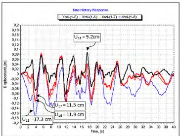
Thus, the following maximum displacements (fig. 6.4) were obtained: U18 = 9.2cm - Acc08, where 1-8
spectral components were removed (i.e. the spectral periods T = 5s ÷ 40s); U17 = 11.5cm - Acc07, where 1-7
spectral components were removed (i.e. the spectral periods T = 5.7s ÷ 40s); U16 = 11.9cm -Acc06, where
1-6 spectral components were removed (i.e. the spectral periods T = 1-6.7s ÷ 40s); U15 = 17.3cm – Acc05,
where 1-5 spectral components were removed (i.e. the spectral periods T = 8s ÷ 40s). According to the purpose of this study it results that the representative accelerogram should be Acc07, that is the original accelerogram from which the periodical spectral periods T > 5s were eliminated. Therefore, we consider that the maximum ground displacement is Dg = 11.5cm. This value is quite close to the value resulted by
applying the Eurocode8 - design code, which gives the value of 10.5cm.
The original and corrected accelerograms - Acc05, Acc06, Acc07 and Acc08 - were used to determine the absolute acceleration and relative displacement response spectra of the critical damping ratio, = 5% (fig. 6.5-6.6). One should note that the acceleration response spectra for the original and corrected accelerogram do not present significant differences. This means that the dynamic results obtained on the basis of these spectra, especially outside isolation range, T < 3s, are not influenced by the initial non-zero velocity and by the incorporated unrealistic long period components (fig. 6.5). Instead, the relative displacement response spectrum from the original accelerogram differs greatly from that of the corrected accelerograms, for spectral periods, T > 5s (fig. 6.6).
Thus, in case of seismic base-isolation analysis the relative displacement response spectra cannot be directly used anymore and making necessary the two corrections analyzed in the paper. Note that the increasing trend of relative displacement response spectrum is small for corrected accelerogram compared with the original accelerogram, being 1-2mm/s, in the first case, compared to 160mm/s in the second case. This conclusion is applicable to both artificial and recorded accelerograms.
Figure 6.1. The acceleration response spectra for critical damping ratio, = 5% on the original accelerogram.
Figure 6.3. The ground displacement calculated from original accelerogram and corrected to the initial velocity, V0 =-0.16m/s.
Figure 6.4. The ground displacement calculated from original and corrected accelerogram.
Figure 6.5. The absolute acceleration response spectra for accelerogram "Orig" and corrected accelerograms.
Figure 6.6. The relative displacement response spectra for accelerogram "Orig" and corrected accelerograms.
7
CONCLUSION
The actual paper identifies and evaluates the
errors in the response of relative displacements for an
oscillating system modelled as a single degree of freedom. The identified errors are: (i) e
rrors resulting from the initial velocity and, (ii) errors generated by long harmonic periods in initial accelerograms. Based on these aspects, an analysis of possible errors in many known recorded accelerograms and their relative displacement response spectrum was performed. In the paper only two cases was presented. The effect of errors on SDOF for the 3s eigen period (usual period for flexible systems or seismically isolated systems) acted by a harmonic ground motion is emphasized. Solutions to correct the errors analyzed in the paper are proposed.Finally, an application to correct a design generated accelerogram was presented to show the effect of taking into consideration of the errors analyzed.
REFERENCES
Ifrim M. 1984. Dinamica structurilor si inginerie seismica. Ed. Did. Si Ped. Bucuresti, Ed. 2.
Cornea, I., Oncescu, M., Marmureanu, G., Balan, F. 1987. Introducere in mecanica fenomenelor seismice si inginerie seismica. Ed. Academia RSR.
Kelly, T. E. 2001. Base Isolation of Structures. Design Guidelines. Holmes Consulting Group Ltd., Rev.0.
Serban V., Androne, M. 2007. Eroare sistematica in programele de calcul si literatura de specialitate referitoare la raspunsul seismic al constructiilor. UTCB.