Performance of the modulation diversity technique for κ μ fading channels

(1)

R E S E A R C H

Open Access

Performance of the modulation diversity

technique for

κ

-

μ

fading channels

Rafael F Lopes

1,3,4*

, Wamberto J L Queiroz

2,3

, Waslon T A Lopes

2,3

and Marcelo S Alencar

2,3

Abstract

The performance of wireless communication systems can be significantly improved using the modulation diversity technique, which is based on the combination of a suitable choice of the reference angle of a signal constellation with independent interleaving of the symbol components. This technique has been evaluated considering different fading channel models, such as Rayleigh, Rice and Nakagami-m. However, in some specific scenarios, the tails of those fading distributions do not properly fit the experimental measured data, which demands the use of more general channel distributions. This article presents a performance evaluation of the modulation diversity technique forκ-μfading channels. New expressions for the PEP (Pairwise Error Probability) are obtained using numerical integration, series representation and upper/lower bounds. The evaluation, based on Monte Carlo simulation, demonstrates that the performance gain of the modulation diversity increases as the fading becomes more severe. Communications channels exhibit some degree of time correlation, which cannot be perfectly estimated, affecting the performance of the modulation diversity system. Thus, a performance evaluation of the system, concerning the presence of temporal correlation and estimation errors in the channel is also presented in the article.

Keywords: Modulation diversity,κ-μfading, Wireless communications

1 Introduction

Multipath fading can signiﬁcantly degrade the perfor-mance of communication systems. Several techniques have been proposed to mitigate the eﬀects of fading to improve their performance, and diversity techniques appear as a solution to the problem [1-3]. Diversity tech-niques provide replicas of the transmitted signals to the receiver [4].

A useful diversity technique is based on the combination of a suitable choice of a reference constellation rotation angle (θ) with the independent interleaving of the symbol components before the transmission [4,5]. The optimal rotation angle depends on the chosen constellation order (M), as well as on the fading severity degree [6]. In this article, this technique is referred to as modulation diver-sity [4,7], but it is also known as constellation rotation [8], signal space diversity [9,10] and rotation and component interleaving diversity [11].

*Correspondence: [email protected]

1D.Sc. Student of the Federal University of Campina Grande (UFCG), Electrical Engineering Post Graduate Program–COPELE, Campina Grande, Brazil 3Institute for Advanced Studies in Communications, Campina Grande, Brazil Full list of author information is available at the end of the article

The performance of the modulation diversity tech-nique has been evaluated considering diﬀerent scenarios, which include M-ary phase shift keying (M-PSK) and

M-ary quadrature amplitude modulation (M-QAM) con-stellations for Rayleigh fading channels [5,7,8,12], Rician fading channels [13,14] and Nakagami-mfading channels [11,15]. However, in some speciﬁc scenarios, the tails of those fading distributions do not properly ﬁt the experi-mental measured data, as discussed in [16].

Yacoub [17] proposed two fading distributions, namely κ-μ and η-μ, to allow flexibility to model the wireless channels fading fluctuations. Those distributions are fully characterized in terms of measurable physical parame-ters. Theκ-μdistribution includes the Rice (Nakagami-n), Nakagami-m, Rayleigh and One-Sided Gaussian distribu-tions as special cases. On the other hand, theη-μ dis-tribution includes the Hoyt (Nakagami-q), Nakagami-m, Rayleigh and One-Sided Gaussian distributions as special cases. As discussed in [17], the versatility provided by the use of those distributions shows a good fit to experimen-tal data (particularly for low values of the fading envelope) [17]. It is worth to mention that this article is focused on

(2)

κ-μdistribution, but the proposed methodology could be extended toη-μdistribution.

Recently, many articles deal with theκ-μandη-μ dis-tributions. Considering the application of diversity tech-niques, useful formulas for the pdf (probability density function) and CDF (Cumulative Distribution Function) of the sum of squared κ-μ variates were presented [18], and an analytical expression for the switching rate of a dual branch selection diversity combiner was derived in [19]. A systematic investigation on the fad-ing characteristics experienced in body to body commu-nications channels, for ﬁre and rescue personnel, was presented in [20], and the parameters κ and μ were obtained for transmission in the 2.45 GHz range. Using a similar approach, the authors in reference [21] inves-tigated the distribution of signal phase in body area networks.

This article presents a performance evaluation of the modulation diversity technique for the κ-μ fading dis-tribution. Novel approximate expressions for the PEP (Pairwise Error Probability) forκ-μ fading channels are derived. Based on the degrees of freedom provided by theκ-μdistribution, the optimum rotation angle and the system performance are evaluated for diﬀerent scenarios, including time correlated channels, subject to estimation errors. It is shown that modulation diversity improves the performance of digital communication systems, especially under severe fading.

The remaining sections are organized as follows. Section 2 presents the system and channel models adopted in this article. An analytical framework for the optimization of modulation diversity technique for κ-μ fading channels is described in Section 3. The perfor-mance evaluation results are presented in Section 4. Section 5 discuss the eﬀects of the temporal correla-tion in the performance of the system, while the results concerning the presence of channel estimation errors are presented in Section 6. Section 7 is devoted to the conclusions.

2 System and channel models

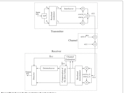
The modulation diversity technique mitigates the eﬀects of the multipath fading in the transmitted signals. In this technique, the introduction of redundancy can be obtained by combining the rotation of the signal constel-lation, by an appropriate reference angleθ, with the inde-pendent interleaving of the symbol components. Figure 1 illustrates the block diagram for the modulation diversity technique [4].

The channel model is characterized by a slowly varying ﬂat fading. Thus, the received signal, denoted byr(t), can be written as

r(t)=α(t)ejφ(t)s(t)+n(t), (1)

in whichs(t)represents the transmitted signal,α(t)is the fading amplitude,φ(t)is the phase shift produced by the channel andn(t) represents the additive noise, modeled as a complex white Gaussian process (AWGN), with zero mean and varianceN0/2 by dimension.

The fading amplitudeα(t)is modeled as aκ-μ station-ary random variable. The κ-μ distribution is a general fading distribution that can be used to represent the small-scale variation of the fading signal in a line-of-sight condition. It is modeled by the parametersκ andμ, that deﬁne the shape of the distribution. Theκ-μdistribution includes Rice (κ = K, μ = 1), Nakagami-m(κ → 0, μ = m), Rayleigh (κ → 0, μ = 1) and One-Sided Gaussian (κ →0,μ=1/2) distributions as special cases [17].

The fading model for theκ-μdistribution considers a signal composed of clusters of multipath waves, propagat-ing in a non-homogeneous environment. The phases of the scattered waves, within each cluster, are random and have similar large delay times. Furthermore, the clusters of multipath waves are assumed to have scattered waves with identical powers, but a dominant component is found within each cluster, which presents an arbitrary power [17].

Theκ-μnormalized probability density function (pdf ) is expressed as [17]

p(α)= 2μ(1+κ)

μ+1 2

κμ−21 _{exp [μκ}_]

αμexp−μ(1+κ)α2

×Iμ−1

2μκ(1+κ)α

, α≥0,

(2)

in which E[α2]= 1, Iν(·) denotes the modified Bessel function of the first kind and orderν([22], 8.431),κ ≥ 0 is the ratio between the total power of the dominant com-ponents and the total power of the scattered waves, and μ > 0 is given byμ = _Var[α1 ₂_]_(1+κ)1+2κ₂. It is assumed that the fading amplitude is perfectly estimated at the receiver, i.e., α(ˆ t) = α(t). Moreover, by coherent detection, the effect of the fading on the phase of the received signal is completely compensated.

For the rotated and interleaved system, the transmitted waveform model can be written as

s(t)= +∞

n=−∞

xnp(t−nTS)cos(ωct)

+ +∞

n=−∞

yn−kp(t−nTS)sin(ωct),

(3)

(t)

φ

^

φ(t) j

Channel Estimation

Compensation of

Input bits

bits

Channel

Output

n(t)

Transmitter

Receiver

(t) e

α

(t)

α^ a_n

b_n y_n

x_n

the phase fading

cos(w t)c

c

sin(w t) cos(w t)c

sin(w t)c

S/P

s(t)

r(t)

Detector

Baseband modulator

Interleaver

Baseband

demodulator

Deinterleaver

Figure 1Block diagram for the modulation diversity technique.

symbol pulse shape,TS is the symbol period, ωc is the carrier frequency and

xn=ancosθ−bnsinθ, (4a)

yn=ansinθ +bncosθ. (4b)

In addition,

an,bn= ±d,±3d,. . .,±( √

M−1)d,

in whichdis the minimum distance between the constel-lation points andMis the modulation order.

Since the transmitted symbols do not share common components, theIandQcomponents are independently aﬀected by fading. Thus, after the deinterleaving, each received symbol vectorrcan be expressed as

r=[rI(t), rQ(t)] , (5)

r=[αI(t)sI(t)+nI(t), αQ(t+k)sQ(t)+nQ(t+k)] , (6)

in which sI(t), sQ(t)are the I and Q signal components of the symbols(t),α_I(t),α_Q(t)represent the fading that

aﬀects the I and Q components, andnI(t),nQ(t)are the I and Q components of noise. Finally, the receiver applies maximum likelihood (ML) metric on the deinterleaved signals to detect the source symbol, as follows

ˆ

s=argmin

s∈S (|r−αs|

2_), ₍₇₎

ˆ

s=argmin s∈S

(|rI(t)−αI(t)sI|2+ |rQ(t)−αQ(t+k)sQ|2), (8)

in which| · |denotes the standard Euclidean norm, rep-resents the component-wise product andSrepresents the signal constellation withMsignals.

3 Optimization analysis of the modulation

(4)

two ways: (a) by using Monte Carlo simulation; or (b) by the optimization of the system SER (Symbol Error Rate) expression.

The first approach requires more computing power than the second one, since many simulations must be per-formed in different settings and with different rotation angles. On the other hand, obtaining an exact closed-form expression for the SER of diversity modulation systems is a difficult problem, and a common approach to evaluate the error probability of a two-dimensional signal constellation is the use of upper bounds, such as the union bound (UB) [23]. Assuming equiprobable symbols, the SER is upper bounded by [12]

in whichSrepresents the signal constellation withM sig-nals andP(s → ˆs)is the pairwise error probability (PEP) andˆsis estimated by the receiver whenshas been trans-mitted (i.e., if|r−αsˆ|2<|r−αs|2). Furthermore, if only the nearest neighbors of each symbol are considered in the performance evaluation,Pecan be approximated by

Pe≈PNNe = Since interleaving is employed for the transmitted sym-bols, the I and Q symbol components experience indepen-dent fading. Letα_I andα_Q be theκ-μdistributed fading amplitudes in the I and Q channels, respectively. Thus, the PEP for a system with modulation diversity, subject toκ-μ fading, is given by [23]

P(s→ ˆs)= Euclidean distances between the symbolssandˆsin the I

and Q components, respectively. The distances are given by

d2_I =[cos(φ1+θ )−cos(φ2+θ )]2, (13) d2_Q=[sin(φ1+θ )−sin(φ2+θ )]2, (14) in which φ1, φ2 represent the phases of the two signal constellation points under consideration.

Applying Craig’s formula for the Q(·) function [24], given by

into (12), the PEP expression becomes

P(s→ ˆs)= 4μ

The integral in (16) can be calculated in diﬀerent ways, as presented in the following sections.

3.1 Exact numerical integration

Different numerical integration techniques can be used to calculate the PEP. In order to make the calculations easier and computationally efficient, the authors have sim-plified (16). After performing the integration in αI and αQ, using the change of variablex = cos2φ and some analytical manipulations, the PEP expression becomes

P(s→ ˆs)= 1 deﬁned function that should be numerically evaluated. This function is deﬁned as

(5)

The function in (18) can be computed using a software package, such as Mathematica, Maple or Matlab.

3.2 Series representation

An alternative form for the PEP can be obtained using a series representation for the Bessel function of the ﬁrst kind in the integrand of (16), which can be expressed by the following expression ([22], 8.445)

Iν(x)=

Introducing (19) into (16), performing the integrations and other analytical manipulations, the PEP expression becomes

in whichF1(·)represents the Appell hypergeometric func-tion ([22], 9.180.1) and B(·) is the Beta function ([22], 8.380.1).

The inﬁnite series form presented in (20) can be trun-cated to a few number of terms, becoming an approxima-tion for the PEP expression. Thus, (20) can be rewritten as

P(s→ ˆs)≥ exp [−2μκ]

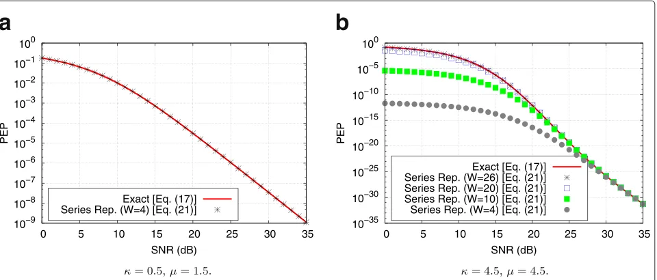
The number of terms in each series (denoted byWand assumed equal in both summations) should be adjusted according to the severity of the fading. Since the PEP approximation is composed of a double summation, a number of W2 terms should be computed. Figure 2 depicts the PEP approximation based on the series rep-resentation considering diﬀerent values of W and the randomly chosen symbols 0.3162+0.9487jand 0.9487− 0.3162j.

As can be seen in Figure 2a, a small number of terms is required to obtain a precise approximation when the channel is characterized by severe fading (κ = 0.5,

μ = 1.5) – in this case, a total number ofW2 = 16 terms is used. However, in a less severe fading scenario (κ =4.5,μ=4.5), as illustrated in Figure 2b, more terms are required for a better precision (in this case, a total number ofW2₌_{676 terms is used).}

An important characteristic of the proposed approxi-mation is that it converges to the exact PEP for high SNR values, even using a small number of terms in the series.

3.3 Lower bounds

A classical approach to derive approximations for analyti-cal functions is the use of bounds. Thus, the authors have derived lower and upper bounds for the PEP expression to be used in the evaluation of the modulation diversity inκ-μfading. In this article, two diﬀerent lower bounds were derived. The ﬁrst lower bound (referred to asLower Bound A) is obtained truncating the PEP series form, pre-sented in (21), to only one term (i.e.,m=0 andn=0). In this case, (21) can be rewritten as

P(s→ ˆs)≥ exp [−2μκ] B

Another lower bound can be derived replacing the exponential functions of (16) by their equivalent power series ([22], (1.211)) and applying ([22], (3.211)). After the analytical manipulations, the PEP function can be rewritten as

(6)

10−9

10−8

10−7

10−6

10−5

10−4

10−3

10−2

10−1

100

0 5 10 15 20 25 30 35

PEP

SNR (dB) Exact [Eq. (17)] Series Rep. (W=4) [Eq. (21)]

a

10−35

10−30

10−25

10−20

10−15

10−10

10−5

100

0 5 10 15 20 25 30 35

PEP

SNR (dB) Exact [Eq. (17)] Series Rep. (W=26) [Eq. (21)] Series Rep. (W=20) [Eq. (21)] Series Rep. (W=10) [Eq. (21)] Series Rep. (W=4) [Eq. (21)]

b

Figure 2Series approximation for the PEP considering the randomly chosen symbols0.3162₊0.9487jand0.9487₋0.3162j.The ﬁgure presents the performance of the series approximation proposed in (20) for the PEP of modulation diversity.

The lower bound presented in (24) is much sim-pler than the one presented in (22), since it does not require the computation of the Appell hypergeometric function.

3.4 Upper bounds

Two PEP upper bounds are proposed to evaluate the modulation diversity system. The ﬁrst upper bound is obtained assuming that (1 + cI) and (1 + cQ) in the denominator of (23) converge, respectively, tocI andcQ at high SNR values, the F1(·) function converges to 1 at high SNR values, and the series become exponen-tial functions. Since, for low SNR values, [(1+cI)(1 + cQ)]μ (cIcQ)μ and [(1+cI)(1+cQ)]

μ

(cIcQ)μ F1(·)

func-tion, then (23) becomes an upper bound and can be rewritten as

Ps→ ˆs≤ B

2μ+ 1₂,1₂ 2πcμ_Icμ_Q

×exp

−μκ

cI 1+cI +

cQ 1+cQ

. (25)

Furthermore, if κ → 0 and μ = m, then (25) coin-cides with the PEP upper bound for Nakagami-mfading channels presented in ([11], Eq.(13)).

The second upper bound is based on the use of the

Chernoﬀ bound (i.e.,Q(x) ≤ 1₂e−x 2

2 _{). It is obtained} sub-stituting the Chernoﬀ bound into (12) and performing the

integration in αI andαQ. Finally, the PEP can be upper bounded by (26)

Ps→ ˆs≤ μ

2μ₍₁₊_κ)2μ

2

×

γd2_I

4 +μ(1+κ)

γd2 Q

4 +μ(1+κ)

−μ

×exp

−γ κμ

d2_I d2

Iγ+4(1+κ)μ

+ d

2 Q

d_Q2γ+4(1+κ)μ

.

(26)

3.5 Performance evaluation of the PEP bounds

The proposed bounds serve as approximations for the PEP function and are used to optimize theθ angle. However, each proposed approximation exhibits a diﬀerent perfor-mance when compared to the exact PEP value, as well as diﬀerent complexity.

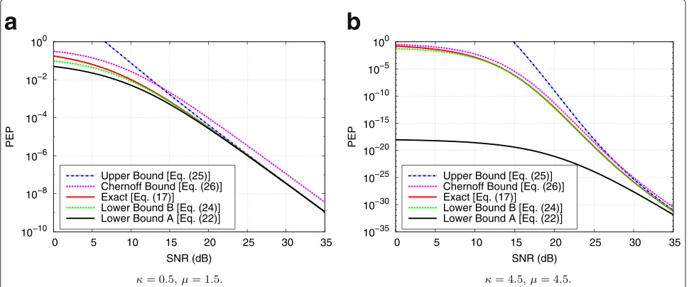
A performance comparison of the proposed lower and upper bounds for the PEP is presented in Figure 3. In the evaluation diﬀerent values ofκ andμand the constella-tion symbols 0.3162+0.9487jand 0.9487−0.3162jare considered.

(7)

10−10

10−8

10−6

10−4

10−2

100

0 5 10 15 20 25 30 35

PEP

SNR (dB) Upper Bound [Eq. (25)] Chernoff Bound [Eq. (26)] Exact [Eq. (17)]

Lower Bound B [Eq. (24)] Lower Bound A [Eq. (22)]

a

10−35

10−30

10−25

10−20

10−15

10−10

10−5

100

0 5 10 15 20 25 30 35

PEP

SNR (dB) Upper Bound [Eq. (25)] Chernoff Bound [Eq. (26)] Exact [Eq. (17)]

Lower Bound B [Eq. (24)] Lower Bound A [Eq. (22)]

b

Figure 3PEP bounds considering the symbols0.3162+0.9487jand0.9487−0.3162j.Figure 3 depicts a comparison among the proposed PEP approximations (namelyUpper Bound,Chernoﬀ Bound,Exact,Lower Bound AandLower Bound B) forκ-μchannels. The same symbols and fading scenarios from Figure 2 are used in Figure 3.

that, whenever a lower bound is used as a PEP approxima-tion, the union bound becomes an approximation and not an upper bound anymore.

4 Results

The adoption of the κ-μfading model allows the eval-uation of communication systems in channel conditions which are not covered by other channel models, such as the Nakagami-m. The ﬂexibility provided by the κ-μ distribution is adequate to evaluate the perfor-mance of modulation diversity. This section presents the performance analysis of the diversity modulation tech-nique for a κ-μ fading channel. Numerical evaluations and Monte Carlo simulations were performed, respec-tively, to optimize the θ angle in (13) and (14), and to verify the gains obtained by the modulation diversity scheme considering diﬀerent channel parameters and PEP expressions.

4.1 Evaluation of the optimum rotation angleθ

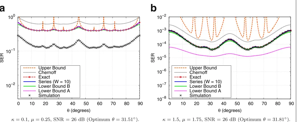
The performance of the modulation diversity technique is directly affected by the constellation rotation angle θ, requiring its optimization, to obtain the value of θ that generates the lowest overall SER. The evaluation of the optimal rotation angle is accomplished by replacing the different PEP expressions in (9). The evaluation was performed considering QPSK and 16-QAM constellations and two different channel scenarios: (a) severe fading con-ditions (κ = 0.1, μ = 0.25) and (b) typical fading conditions (κ=1.5,μ=1.75) [25].

Figures 4 and 5 depict the SER of the modulation diver-sity system (with QPSK and 16-QAM constellations) for

aκ-μfading channel. As can be seen in the ﬁgures, the optimal angle depends on the constellation order and the channel characteristics. Moreover, the SER curves are symmetric with respect to the angle 45◦, since analogous constellations are generated regardless of the rotation direction (i.e., clockwise or counterclockwise).

Comparing Figures 4 and 5, one can note that the overall performance of the PEP approximations depends on the fading parameters κ and μ. For severe chan-nel conditions (i.e., Figures 4a and 5a), the Cher-noﬀ bound presents the worst performance considering the SER approximation. One can note that the other bounds exhibit a similar performance to theExact PEP calculation.

On the other hand, in typical fading scenarios (i.e., Figures 4b and 5b), the upper bound shown in (25) performs worse than the Chernoﬀ bound. The Exact,

Series and Simulation curves are indistinguishable, and theLower Bound Bcurve is very close to them. Finally, the

Lower Bound Aapproximation has the worst performance when compared to theExactPEP.

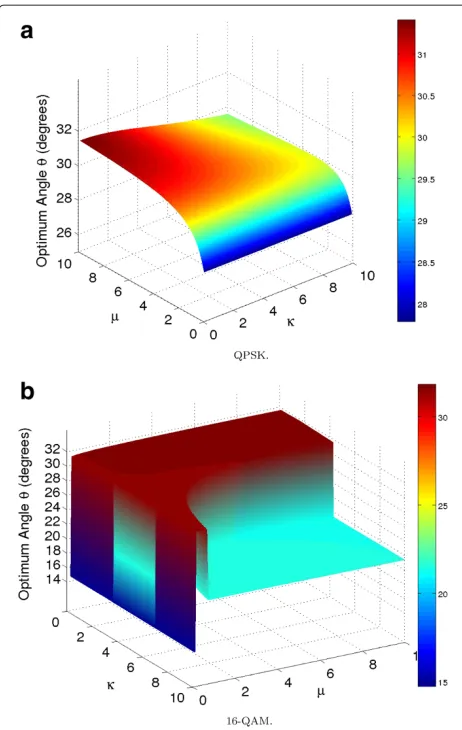
An overview of the optimum rotation angle in modu-lation diversity systems subject to κ-μ fading is shown in Figure 6 which contains the curves of the optimal θ as a function of the parametersκ andμand considering the use of QPSK and 16-QAM constellations, respec-tively. The optimization process was conducted using the

Lower Bound Bapproximation, due to its simplicity and accuracy.

(8)

10−2

10−1

100

0 10 20 30 40 50 60 70 80 90

SER

θ (degrees)

Upper Bound Chernoff Exact Series (W = 10) Lower Bound B Lower Bound A Simulation

a

10−8

10−7

10−6

10−5

10−4

10−3

10−2

0 10 20 30 40 50 60 70 80 90

SER

θ (degrees)

b

Figure 4SER of the QPSK modulation diversity system as a function of the rotation angleθ.The simulated and approximated SER values for a modulation diversity system (with QPSK) are shown in the ﬁgure. Two fading scenarios were used in the evaluation:(a)severe fading (κ=0.1,

μ=0.25) and(b)typical fading (κ=1.5,μ=1.75). The fading scenarios were evaluated for an SNR=20 dB.

at high values of μand low values of κ (i.e., the fading conditions are less severe). In contrast, the lowest opti-mum angle value (27.8◦) should be used for lowκandμ values (i.e., in very severe channel fading). Furthermore, other intermediate values should be selected according to the channel fading conditions, using the results shown in Figure 6a.

Figure 6b presents the optimum rotation angle θ for the 16-QAM constellations as a function of the chan-nel fading parameters. As shown in the ﬁgure, there are abrupt transitions in the graphic, the result of small changes in the minimum values of the system SER (i.e.,

minor changes in the sidelobes of the SER curves—refer to Figure 5).

If a Nakagami-m channel fading model is considered (i.e.,κ → 0 andμ = m), the optimumθ values are con-ﬁrmed by the values presented in ([11], Table one) (for QPSK constellations), which conﬁrms the precision of the

Lower Bound Bapproximation.

4.2 Evaluation of the execution time

In addition to the SER evaluation, the authors evalu-ated the average execution time of 900 union bound calculations, considering the diﬀerent proposed PEP

10−2

10−1

100

0 10 20 30 40 50 60 70 80 90

SER

θ (degrees)

a

10−8

10−7

10−6

10−5

10−4

10−3

10−2

0 10 20 30 40 50 60 70 80 90

SER

θ (degrees)

b

(9)

Figure 6Optimum angleθas a function of diﬀerent channel fading parameters.The evaluation was performed using the proposedLower Bound BPEP approximation (presented in (24)).

approximations. Furthermore, each round of the experi-ment was executed 30 times, in order to provide statis-tical inferences. Table 1 shows the execution times for the QPSK and 16-QAM union bounds considering the proposed PEP expressions.

As can be seen in the table, considering the most accu-rate approximations (as discussed in Section 4.1), the

Lower Bound Bpresented the lowest execution time. Its running time is slightly above the Chernoﬀ and Upper Bound approximations, but presents an improved accu-racy, and is attractive to use in the rotation optimization process.

4.3 Evaluation of the System Symbol Error Rate

Based on the use of the of theLower Bound B approx-imation, this section presents the SER evaluation of communication systems that use the modulation diver-sity technique for κ-μ fading channels. Monte Carlo

Table 1 Average execution time for 900 calculations of the union bound considering the proposed PEP

approximations

Constellation Fading PEP expression Exec. time (sec.)

QPSK Severe Upper bound 0.020

Chernoﬀ 0.022

Exact 0.922

Series 148.490

Lower bound A 1.064

Lower bound B 0.023

Typical Upper bound 0.026

Chernoﬀ 0.019

Exact 1.701

Series 168.540

Lower bound A 1.985

Lower bound B 0.031

16-QAM Severe Upper bound 0.170

Chernoﬀ 0.124

Exact 17.924

Series 2956.030

Lower bound A 20.827

Lower bound B 0.167

Typical Upper bound 0.172

Chernoﬀ 0.126

Exact 30.335

Series 3226.570

Lower bound A 34.965

Lower bound B 0.187

Table 1 presents the average execution time for 900 calculations of the union bound considering the proposed PEP approximations and simulations. Two fading scenarios were used in the evaluation:(a)severe fading (κ₌0.1,

μ=0.25) and(b)typical fading (κ=1.5,μ=1.75).

simulations were performed to evaluate the eﬃciency as modulation diversity is used for fading. The sys-tem dynamically adapts the rotation angle according to the channel SNR using the golden section search method ([26], Section 10.2). The same channel and system parameters used in the experiments of Section 4.1 were adopted (Figures 4 and 5).

(10)

10−3 10−2 10−1 100

0 5 10 15 20 25 30 35 40

SER

SNR (dB) Union Bound − exact PEP Nearest Neighbor − Lower Bound B Simulation − without rotation Simulation − with rotation

10−6 10−5 10−4 10−3 10−2 10−1 100

0 5 10 15 20

SER

a

b

Figure 7SER of a QPSK system with and without rotation in severe and typical fading conditions.

In a conventional transmission, the fading peaks can completely degrade the information of the transmitted symbols (in-phase and quadrature components). How-ever, using the modulation diversity technique, the symbol components are transmitted at different instants of time, creating a redundancy between those components. In this context, the gain provided by the modulation diversity is higher under severe fading conditions, but it does not affect the system performance when the signals are trans-mitted in AWGN channels, since the Euclidean distance between the symbols remains constant regardless of the rotation angleθ. This aspect can be verified in Figures 7 and 8, the rotated constellation outperforms the refer-ence system (i.e., without rotation). However, one can note that the gain provided by this technique decreases as the fading severity is reduced (i.e., as the values ofκ andμ are increased).

For the QPSK system, the modulation diversity gain is 16.86 dB (for a SER of 4.35× 10−2) considering severe fading conditions (κ = 0.1, μ = 0.25), and is 4.80 dB (for a SER of 4.04 × 10−4) in a typical fading scenario (κ = 1.5,μ=1.75). On the other hand, for the 16-QAM system, a gain of 11.28 dB (for a SER of 9.30×10−2) is obtained in severe fading, while in typical fading, the mod-ulation diversity system has a gain of 3.74 dB (for a SER of 1.34×10−3).

Another important aspect to note is that the union bound is not a good approximation for channels sub-ject to severe fading conditions, but it becomes a suitable approximation for better channel conditions. Instead, the nearest neighbor, with the Lower Bound B PEP, ﬁts well in severe fading (e.g., Figure 7a), but becomes a lower bound in typical fading scenario (e.g., Figure 7b).

10−2 10−1 100

0 5 10 15 20 25 30 35 40

SER

10−5 10−4 10−3 10−2 10−1 100

0 5 10 15 20 25

SER

a

b

(11)

5 Performance evaluation of the modulation diversity technique in time correlated channels The previous evaluation of the modulation diversity tech-nique considered that the in-phase (I) and quadrature (Q) components are independently affected by the fading. That assumption is based on the fact that the interleaving depth (i.e., the temporal shift between a pair of inter-leaved symbols, denoted byk) is larger than the channel coherence bandwidth. However, in an actual scenario, the channel conditions constantly change, and the perfect channel state information may not be available, preventing the system from dynamically adapt the interleaving depth. Moreover, the coherence bandwidth changes according to the Doppler frequency, which depends on the relative velocity between the transmitter and the receiver. There-fore, some degree of temporal correlation between the fading coefficients appears, affecting the performance of the modulation diversity technique.

This section presents an evaluation of the modulation diversity assuming a time correlated channel. An analysis of the inﬂuence of the correlation on the rotation angle and on the performance of the technique is also shown.

5.1 Generation of a time correlatedκ-μfading channel The ﬁrst challenge to be faced in the proposed evalua-tion is the generaevalua-tion of a time correlatedκ-μfading. The developedκ-μtime correlated fading generator is based on the adaptation of the classical time correlated Rayleigh fading generator, on the properties of the Gaussian pro-cesses and on theκ-μfading physical model.

According that model [17], the received signal is a composition of multiple clusters, each one consisting of scattered waves of identical powers and of a dominant component of arbitrary power. Thus, the envelopeRof the κ-μdistribution can be deﬁned in terms of its in-phase and quadrature components, as follows

R2=

in which Xi and Yi are independent Gaussian random processes with meansE[Xi]= E[Yi]= 0 and variances V[Xi]=V[Yi]=σ2,piandqiare, respectively, the mean values of the in-phase and quadrature components of the

ith cluster andnis the number of clusters.

As discussed in Section 2, the parametersκandμdeﬁne the shape of the distribution, withκrepresenting the ratio between the total power of the dominant components and the total power of the scattered components, analytically deﬁned as follows [17]

κ =

The parameterμ extends the original meaning of the parameternto include some speciﬁc channel character-istics, such as [17]: (a) non-zero correlation among the clusters of multipath components; (b) non-zero correla-tion between the in-phase and quadrature components within each cluster; and (c) the non-Gaussian nature of the in-phase and quadrature components of each cluster of the fading signal, among other characteristics.

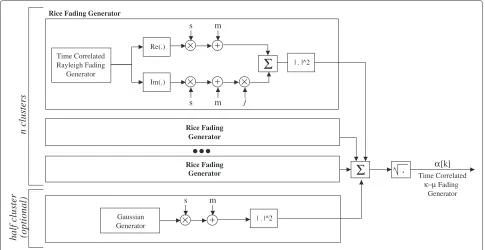
Based on the physical model of theκ-μchannel, Figure 9 presents the block diagram of the proposed fading gener-ator (withpi,qi = m,∀1≤i ≤n). As can be seen in the ﬁgure, the resultant correlatedκ-μprocess is composed by a sum ofncorrelated Rician processes (with each pro-cess representing a cluster of multipath waves, containing a dominant component).

The ﬁrst step performed by the proposed system is the generation of a time correlated Rayleigh fading. Diﬀer-ent techniques are available in the literature to generate time correlated Rayleigh fading channels, including the well-known techniques of Smith spectrum [27] and sum of sinusoids [28]. The corresponding normalized autocor-relation function for the Rayleigh fading is given by [29]

R(τ )=J0(2πfDτ ), (30)

in which τ is the time shift delay and fD is the maxi-mum Doppler frequency. The power spectrum density of a time-correlated Rayleigh fading is given by the classical Jake’s Doppler spectrum [27,30], as follows

S(f)=

in which f is the frequency shift relative to the carrier frequency.

The Rayleigh random variable is transformed, by a suitable function, to produce the Rice fading. Since the Rayleigh fading is a circularly symmetric Gaussian pro-cess, its statistics can be modiﬁed, without losing its Gaussian characteristics. Thus, the Rice fading is obtained from the complex Gaussian processα=X+jY, in which the real and imaginary components have mean m and standard deviations, i.e.,X,Y∼N(m,s2), given by [31]

(12)

Rice Fading Generator

Im(.)

Σ

Re(.)

| . |^2

Generator Rayleigh Fading Time Correlated

Rice Fading Generator

| . |^2 Generator

Gaussian

(optional)

half cluster

Σ

.

Fading κ−μ

Generator Time Correlated

α[k]

n clusters

s

s j

Rice Fading Generator

s

m

Figure 9Block diagram of the time correlatedκ-μfading envelope generator.

K = 0 corresponds to a Rayleigh fading channel and

K → ∞ corresponds to a non-fading (i.e., constant) channel.

The Rice fading generation process must be repeatedn

times, withnbeing the corresponding integer value of the channel parameterμ. An optional Gaussian generator can be used for half-integer values of the parameterμ.

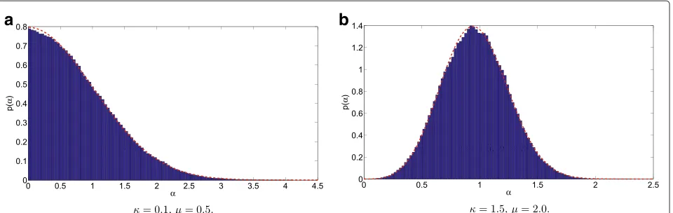
This limitation requires the adaptation of the previously used channel scenarios to new values, as follows: (a) the severe fading conditions (κ =0.1,μ=0.5) and (b) typical fading conditions (κ=1.5,μ=2.0).

Finally, the squared norm of the Rician processes are added and a square root is applied to generate the time correlated κ-μ process. A normalization of the fading samples is also required.

Figure 10 presents the histograms of the envelopes for the twoκ-μfading scenarios (generated using the devel-oped system) and their corresponding theoretical pdfs. As can be seen, the histograms ﬁt well with the theoretical pdfs.

The normalized autocorrelation function, for both sce-narios, was calculated using the generated fading samples. Figure 11 shows the autocorrelation for the fading sce-narios, considering a sampling frequency of 270833 sym-bols/second (analogous to the one used in GSM–Global System for Mobile Communications), and two diﬀerent Doppler frequencies.

As expected, the presence of dominant components and a non-unitary number of clusters (i.e., determined byμ),

create a correlation among the fading samples. As a result, the channel does not become uncorrelated (instead, the correlation reduces or increases according to the tempo-ral separation of the samples). Finally, the generated fading samples are ready to be used for the evaluation of the modulation diversity technique.

5.2 Performance over time correlated channel

The overall performance of the modulation diversity tech-nique for uncorrelated channels is only affected by the rotation angle of the signal constellation (that must be defined according to the channel characteristics). Corre-lated channels require that the interleaving depthkshould be carefully defined, to reduce the correlation between the interleaved channel fading samples. Therefore, the smaller the maximum Doppler frequencyfD, the larger should be the interleaving depth, requiring the analysis of the effect of the change in the interleaving depth.

Figure 12 presents the Bit Error Rate (BER) curves for a 16-QAM system as a function of the interleaving depth

(13)

a

b

Figure 10Histograms of two generatedκ-μfading channels and their corresponding theoretical pdfs (represented by the red dashed lines).

considered in the evaluation. The rotation angle for each scenario was optimized using the union bound with the proposed PEP approximationLower Bound B(presented in (24)).

As can be seen in the ﬁgures, in correlated channels, the BER of the system with modulation diversity changes with the interleaving depth. The BER reduces as the cor-relation between the interleaved symbols also reduces. For instance, the minimum BER in Figure 12a is achieved when thekvalue is approximately 1650 symbols (which is equivalent to the smallest correlation value in Figure 11b,

fD=100 Hz). Similarly, in Figure 12b, the minimum BER is obtained whenkis approximately 825 symbols (which is equivalent to the smallest correlation value in Figure 11b,

fD = 200 Hz, and the double of the 100 Hz scenario). An important characteristic to be noted in the presented curves is that, for the minimum correlation points, the

BER of time correlated channels is smaller than the value obtained for uncorrelated channels.

In the absence of rotation (0.0◦), the system becomes invariant to changes in the interleaving depth, since there is no redundancy between the I and Q interleaved components of the transmitted symbols. Finally, a chan-nel without time correlation is equivalent to a chanchan-nel with fD→ ∞ (i.e., any pair of interleaved symbols is uncorrelated). Since the correlation among the transmit-ted symbols is null, the interleaving depth k also does not aﬀect the performance of the modulation diversity system.

The system BER was evaluated as a function of the rota-tion angle, to access the inﬂuence of the time correlarota-tion in the optimum rotation angle. Figure 13 illustrates the obtained curves for a 16-QAM system subject to a typical fading scenario (κ =1.5,μ=2.0), a sampling frequency

0.6 0.65 0.7 0.75 0.8 0.85 0.9 0.95 1

0 512 1024 1536 2048 2560 3072 3584 4096 4608 5120

A

utocorrelation

Time, in symbol intervals f_D = 100 Hz f_D = 200 Hz

0.65 0.7 0.75 0.8 0.85 0.9 0.95 1

0 1024 2048 3072 4096 5120 6144 7168 8192 9216 10240

A

utocorrelation

Time, in symbol intervals f_D = 100 Hz f_D = 200 Hz

a

b

(14)

10−10 10−9 10−8 10−7 10−6 10−5 10−4 10−3 10−2 10−1

500 1000 1500 2000 2500

BER

Interleaving depth (k)

θ=0.0°, E_b/N₀=10dB

θ=45.0°, E_b/N₀=10dB (uncorrelated)

θ=45.0°, E_b/N₀=10dB

θ=0.0°, E_b/N₀=15dB

θ=30.2°, E_b/N₀=15dB

θ=0.0°, E_b/N₀=20dB

θ=30.2°, E_b/N₀=20dB

10−10 10−9 10−8 10−7 10−6 10−5 10−4 10−3 10−2 10−1

500 1000 1500 2000 2500

BER

Interleaving depth (k)

θ=0.0°, E_b/N₀=10dB

θ=45.0°, E_b/N₀=10dB

θ=0.0°, E_b/N₀=15dB

θ=30.2°, E_b/N₀=15dB

θ=0.0°, E_b/N₀=20dB

θ=30.2°, E_b/N₀=20dB

a

b

Figure 12BER of the modulation diversity system as a function of the interleaving depth considering a 16-QAM system in a typical fading scenario (κ=1.5,μ=2.0), a sampling frequency of 270833 symbols/second and three diﬀerent values of SNR (10, 15, and 20 dB).

of 270833 symbols/second, an SNR of 20 dB, diﬀerent maximum Doppler frequencies and interleaving depths.

The performance of the system forfD=100 Hz andk= 1650 is equivalent to the performance forfD=200 Hz and k = 825, since in both scenarios the system experiment the same correlation level. The ﬁgure shows the absence of signiﬁcant variations in the value of the optimum angle between correlated and uncorrelated channels. Further-more, as discussed earlier, for the minimum correlation points, the system BER for time correlated channels is smaller than the value obtained for uncorrelated channels. Finally, Figure 14 shows the BER curves of the mod-ulation diversity as a function of the SNR. The rotation angle used in that evaluation was obtained averaging the

10−7 10−6 10−5 10−4 10−3

0 10 20 30 40 50 60 70 80 90

BER

θ Angle

Uncorrelated, SNR = 20 dB f_D = 100 Hz, SNR = 20 dB, k = 1650 f_D = 200 Hz, SNR = 20 dB, k = 825

Figure 13BER of the modulation diversity system as a function of the rotation angle.The evaluation was performed considering a 16-QAM system under a typical fading scenario (κ=1.5,μ=2.0), a sampling frequency of 270833 symbols/second, an SNR of 20 dB and diﬀerent maximum Doppler frequencies.

optimum rotation angles presented in Figure 12. In the experiments, a 16-QAM system subject to a typical fad-ing scenario (κ =1.5,μ=2.0), and a sampling frequency of 270833 symbols/second (for a time correlated chan-nel) were considered. Similar results were obtained for

fD = 100 Hz andk = 1650, and forfD = 200 Hz and k=825, therefore, only one curve is shown in the ﬁgure.

The addition of modulation diversity gives a gain improvement of 5.7 dB (for a BER of 10−5). However, the system gain increases when correlated channels are con-sidered and an appropriate value of k is deﬁned, which represents an additional gain of approximately 1 dB when compared to the uncorrelated channel scenario (for the same BER value).

10−6 10−5 10−4 10−3 10−2 10−1 100

0 5 10 15 20

BER

SNR (dB)

θ=0.0° (uncorrelated)

θ=35.1° (uncorrelated)

θ=35.1° (time correlated)

(15)

Based on the experiments, one concludes that, for time correlated channels, the interleaving depth must be care-fully deﬁned to improve the overall system performance. The correct choice of the interleaving depth reduces the system BER to lower values than the obtained in uncor-related channels (i.e., channels withfD → ∞). Another consequence of using the optimum interleaving depth is that there are no signiﬁcant changes in the optimum rotation angle.

6 Performance evaluation of the modulation

diversity technique subject to channel estimation errors

In the previous sections, the performance of the mod-ulation diversity system was evaluated considering the existence of ideal channel state information (CSI), i.e., the channel gain is perfectly known. In a practical imple-mentation, the channel gain is not known and should be estimated at the receiver. The estimated values are used to compensate the fading eﬀects on the received symbols. However, the larger the system error estimation, the larger the degradation in performance of the communication system.

Monte Carlo simulation was conducted to verify the inﬂuence of the estimation errors on the performance of the modulation diversity. Those experiments aim to investigate the impact of using classical channel amplitude and phase estimation algorithms on the optimum rotation angle value and on the overall system performance.

An analysis of the impact of the estimation errors on the modulation diversity system, as well as the results of the experiments are presented in this section. The least mean square (LMS) and the ﬁrst order phase-locked loop (PLL) [32] algorithms, adopted to track the amplitude and phase of the wireless communication channel, are also described.

6.1 Estimation algorithms

The estimation algorithms are used to track the amplitude and phase of the channel impulse response. This allows the system to compensate the eﬀects of the fading in the received signals, improving the overall performance. This section presents two estimators: (a) LMS, for amplitude estimation and (b) PLL, for phase estimation.

6.1.1 Amplitude estimator

In the evaluation, the LMS algorithm was used to esti-mate the amplitude of the channel impulse response. The algorithm operates by using a recursive relation, that continuously updates the estimated channel amplitude

ˆ

α(n), as follows [32]

ˆ

α(n+1)= ˆα(n)+λs(n)e∗(n), (34)

in which λ is the step-size parameter of the LMS algorithm,(·)∗is the complex conjugate operator ande(n) is the error signal given by

e(n)=r(n)− ˆα(n)ˆs(s), (35)

in whichr(n)is thenth received signal sample,αˆnis the nth estimated fading amplitude sample andˆs(s)is thenth estimated transmitted signal. During the training process ˆ

s(s) =s(s). After the training process, the signal estimate is provided by the detector.

6.1.2 Phase estimator

Since the performance of the modulation diversity is aﬀected by the constellation rotation angle, the channel phase estimation becomes a crucial aspect to be han-dled in the system. For the evaluation a ﬁrst order PLL algorithm was used.

Similarly to the LMS algorithm, the PLL uses a recursive ﬁlter in the estimation. The phase updating is performed using the following expression

ˆ

φ(n+1)= ˆφ(n)+ρuφ(n), (36)

in whichρ is the step of the recursive ﬁlter anduφ(n)is the phase error detector, given by [33]

uφ(n)=Im[e−jφˆs∗(n)r(n)] . (37)

The PLL algorithm aims to maximize the phase likeli-hood function, which is obtained when the output of the phase error detector is zero. A more complete description of the PLL algorithm can be found in [33].

6.2 Evaluation of the optimum rotation angle considering channel estimation errors

In actual communication systems, the fading estimation algorithms are unable to perfectly track the amplitude and phase of the channel impulse response. The presence of estimation errors degrades the performance of the modu-lation diversity, as well as aﬀects the value of the optimum rotation angle.

The fading estimation is independently performed on each block of symbols (using a training sequence trans-mitted at the beginning of each block). The larger the size of the training sequence, the better the performance of the estimator (at the cost of a reduction in the sys-tem throughput). In the performed evaluation, 20% of each block of symbols consists of training symbols (sim-ilar to the value adopted in the GSM system, that uses approximately 17.6% of the block size for training).

(16)

Table 2 Values of the steps of LMS (λ) and PLL (ρ) for diﬀerent scenarios

Scenario 1(κ=0.1,μ=0.5) 100 Hz 200 Hz

M=4 θ=0.0◦ λ 0.5 0.5

ρ 0.5 0.5

θ=29.2◦ λ 0.25 0.25

ρ 0.25 0.45

M=16 θ=0.0◦ λ 0.35 0.5

ρ 0.3 0.5

θ=10.7◦ λ 0.5 0.6

ρ 0.35 0.5

Scenario 2 (κ=1.5,μ=2.0) 100 Hz 200 Hz

M=4 θ=0.0◦ λ 0.85 0.5

ρ 0.3 0.8

θ=41.0◦ λ 0.1 0.2

ρ 0.25 0.45

M=16 θ=0.0◦ λ 0.1 0.2

ρ 0.7 0.8

θ=35.1◦ λ 0.15 0.2

ρ 0.4 0.5

Table 2 shows the optimized values of the parameters of the LMS and PLL algorithms (λandρ). The step-size parameters were deﬁned by computer simulation, to reduce the system BER. In the experiments, the optimization ofλ

(LMS) was performed assuming that the phase is perfectly estimated, and the optimization ofρ(PLL) considered the amplitude perfectly estimated.

ofρ(PLL) considered the amplitude perfectly estimated. Table 2 shows the values obtained for the step parameters in diﬀerent scenarios.

Based on the optimized values of λ and ρ, Monte Carlo simulation was performed to evaluate the impact of

channel estimation errors on the optimal rotation angle. Figure 15 presents the BER curves of the modulation diversity system as a function of the rotation angle, consid-ering diﬀerent parameters for the estimation algorithms (LMS and PLL), a 16-QAM system under a typical fad-ing scenario (κ = 1.5,μ = 2.0), a sampling frequency of 270833 symbols/second, an SNR of 20 dB and 100 Hz of maximum Doppler frequency.

As can be seen in the figure, the presence of channel estimation errors modifies significantly the value of the optimum rotation angle, requiring that the optimization ofθ considers the existence of errors in the estimation of channel amplitude and phase. However, to evaluate the efficiency of the modulation diversity when operating in the presence of estimation errors, in the following exper-iments, the same rotation angles obtained for perfectly estimated channels are used. Thus, the simulation results, considering the impact of channel estimation errors on the system BER (as a function of the channel SNR), are presented in Figure 16. The curves with rotation were gen-erated using an interleaving depth of 1650 symbols for

fD = 100 Hz and 825 symbols forfD = 200 Hz. The per-formance curves with the absence of channel estimation errors were also included for comparison.

Although the estimation errors have modiﬁed the opti-mum value of θ, the use of the modulation diversity technique have improved the performance of the QPSK system (fD = 100 Hz) when compared to conventional systems (i.e., systems that do not use this technique, or 0.0◦), as can be seen in Figure 16a. As can be seen in the ﬁgure, the rotated scheme outperforms the conven-tional system by approximately 3.65 dB for a BER value of 4.13×105_.

10−8 10−7 10−6 10−5 10−4 10−3 10−2 10−1 100

0 10 20 30 40 50 60 70 80 90

BER

θ Angle

λ=1.0

λ=0.2

λ=0.15 Perfect Estimation

10−7 10−6 10−5 10−4 10−3 10−2

0 10 20 30 40 50 60 70 80 90

BER

θ Angle

ρ=1.0

ρ=0.4

ρ=0.2 Perfect Estimation

a

b

(17)

10−6 10−5 10−4 10−3 10−2 10−1 100

0 5 10 15 20

BER

SNR (dB)

θ=0.0° (Perfect estimation)

θ=0.0° (LMS+PLL), 100 Hz

θ=41.0° (LMS+PLL), 100 Hz

θ=0.0° (LMS+PLL), 200 Hz

θ=41.0° (LMS+PLL), 200 Hz

10−6 10−5 10−4 10−3 10−2 10−1 100

0 5 10 15 20 25 30

BER

SNR (dB)

θ=0.0° (LMS+PLL), 100 Hz

θ=35.1° (LMS+PLL), 100 Hz

θ=0.0° (LMS+PLL), 200 Hz

θ=35.1° (LMS+PLL), 200 Hz

a

b

Figure 16BER of the modulation diversity system, subject to amplitude and phase estimation errors, as a function of the channel SNR. The evaluation was performed considering a QPSK and a 16-QAM system under a typical fading scenario (κ=1.5,μ=2.0), a sampling frequency of 270833 symbols/second and maximum Doppler frequencies of 100 and 200 Hz.

However, the same conclusion cannot be obtained if a 16-QAM system is considered (Figure 16b). Instead, the use of a non-optimal rotation angle (35.1◦) has sig-niﬁcantly degraded the performance of the conventional system (0.0◦). The degradation caused by the incorrect choice of the rotation angle can be conﬁrmed compar-ing the BER for bothθ values in Figure 15. For a BER of 6.3×10−4, a loss of approximately 12.92 dB is observed when comparing the rotated and unrotated systems.

Finally, as a consequence of the presence of channel esti-mation errors in correlated fast fading channels, a bit error rate ﬂoor appear in the curves. The error ﬂoor increases with the value of the maximum Doppler frequency (fD). That happens because, for higher values offD, the channel variations are faster, increasing the number of estimation errors generated by LMS and PLL algorithms.

7 Conclusions and future research

The used fading models provide ﬂexibility to characterize wireless channels in terms of measurable physical param-eters. The recently proposedκ-μmodel is a general fading distribution that can be used to represent the small-scale variation of the fading signal in a line-of-sight condition. The versatility obtained with the use of theκ-μ distribu-tion provides a good ﬁt to experimental data (particularly for low values of the fading envelope).

Diversity techniques are important resources to miti-gate the eﬀect of fading in wireless communications. Mod-ulation diversity represents a relevant technique which combines a reference constellation rotation angleθ with the independent interleaving of the symbol components.

This article presented a performance evaluation of the modulation diversity technique forκ-μfading channels.

To the best of authors’ knowledge, the performance of the modulation diversity technique has not been evaluated considering theκ-μfading model. Novel expressions to calculate the PEP of modulation diversity systems subject toκ-μfading are derived, and they are numerically evalu-ated and compared. Finally, Monte Carlo simulations were used to evaluate the performance of the modulation diver-sity technique and to compare communication systems with and without this technique.

In actual systems, the performance of the modulation diversity can be affected by different impairments, such as the temporal correlation and the presence of estima-tion errors. Thus, different evaluaestima-tions were performed in order to verify the impact of those impairments in the performance of the system.

When evaluating the modulation diversity in corre-lated channels, the authors have concluded that, if the interleaving depth is appropriately deﬁned, the overall system performance is improved in correlated channels. The correct choice of the interleaving depth reduces the system BER to lower values than the obtained in uncor-related channels (i.e., channels withfD → ∞). Further-more, the use of the optimal interleaving depth does not cause signiﬁcant changes in the optimum rotation angle.

(18)

Finally, the authors have veriﬁed that in the correlated channels, the estimation errors create a bit error rate ﬂoor, whose values increase with the value of the maximum Doppler frequency (fD).

Future research includes the evaluation of the modu-lation diversity technique in η-μ fading channels. The authors also intend to develop closed-form form expres-sions or more accurate approximations for the symbol error probability of those systems.

Endnote

a_{The value of the}_F

1(·)function in (23) is greater than or equal to 1.

Competing interests

The authors declare that they have no competing interests.

Acknowledgements

The authors would like to thank COPELE/UFCG, Fapema, Federal Institute of Maranh˜ao (IFMA), Iecom and Capes for supporting the development of this research.

Author details

1_{D.Sc. Student of the Federal University of Campina Grande (UFCG), Electrical} Engineering Post Graduate Program–COPELE, Campina Grande, Brazil. 2_{Department of Electrical Engineering, Federal University of Campina Grande,} Campina Grande, Brazil.3Institute for Advanced Studies in Communications, Campina Grande, Brazil.4_{Federal Institute of Maranh˜ao, S˜ao Lu´ıs, Brazil.}

Received: 21 March 2012 Accepted: 8 January 2013 Published: 29 January 2013

References

1. VM DaSilva, ES Sousa, Fading-resistant modulation using several transmitter antennas. IEEE Trans. Commun.45(10), 1236–1244 (1997) 2. GJ Foschini, MJ Gans, On limits of wireless communications in a fading

environment when using multiple antennas. Wirel. Personal Commun.6, 311–335 (1998). http://dx.doi.org/10.1023/A:1008889222784

3. V Tarokh, N Seshadri, AR Calderbank, Space-time codes for high data rate wireless communication: performance criterion and code construction. IEEE Trans. Inf. Theory.44(2), 744–765 (1998)

4. WTA Lopes, F Madeiro, JF Galdino, MS Alencar, inProceedings of the 64th IEEE Vehicular Technology Conference 2006 Fall (VTC’2006Fall), vol. 1. Impact of the estimation errors and Doppler eﬀect on the modulation diversity technique, Montr´eal, Canada, 2006), pp. 1–5

5. SB Slimane, An improved PSK scheme for fading channels. IEEE Trans. Veh. Technol.47(2), 703–710 (1998)

6. DP Andrez-Calder ´on, AC Oria, J Garc´ıa, P L ´opez, V Baena, I Lacadena, in XXIV Conference on Design of Circuits and Integrated Systems. Rotated constellation for DVB-T2, Zaragoza, Spain, 2009). http://dcis2009.unizar. es/index.php

7. G Taricco, E Viterbo, Performance of component interleaved signal sets for fading channels. IEE Electron. Lett.32(13), 1170–1172 (1996) 8. MN Khormuji, UH Rizvi, GJM Janssen, SB Slimane, in10th IEEE Singapore

International Conference on Communication systems, vol. 1. Rotation optimization for MPSK/MQAM signal constellations over Rayleigh fading channels, Singapore, 2006), pp. 1–5

9. J Boutros, E Viterbo, Signal space diversity: a power- and

bandwidth-eﬃcient diversity technique for the Rayleigh fading channel. IEEE Trans. Inf. Theory.44(4), 1453–1467 (1998)

10. J Kim, I Lee, inIEEE International Conference on Communications, vol. 1. Analysis of symbol error rates for signal space diversity in Rayleigh fading channels, Beijing, China, 2008), pp. 4621–4625

11. A Yilmaz, O Kucur, Performance of rotated PSK modulation in Nakagami-m fading channels. Elsevier Digital Signal Process.21(2), 296–306 (2011). http://www.sciencedirect.com/science/article/pii/S105120041000151X

12. NF Kiyani, JH Weber, AG Zajic, GL Stuber, inIEEE 68th Vehicular Technology Conference (VTC 2008-Fall), vol. 1. Performance analysis of a system using coordinate interleaving and constellation rotation in Rayleigh fading channels, Calgary, Canada, 2008), pp. 1–5

13. S Ozyurt, O Kucur, I Altunbas, Error performance of rotated phase shift keying modulation over fading channels. Wirel. Personal Commun.43, 1453–1463 (2007). http://dx.doi.org/10.1007/s11277-007-9319-7 14. J Kim, W Lee, J-K Kim, I Lee, On the symbol error rates for signal space

diversity schemes over a Rician fading channel. IEEE Trans. Commun. 57(8), 2204–2209 (2009)

15. NF Kiyani, JH Weber, inIEEE Global Telecommunications Conference, vol. 1. Performance analysis of a partially coherent system using constellation rotation and coordinate interleaving, New Orleans, USA, 2008), pp. 1–5 16. S Stein, Fading channel issues in system engineering. IEEE J. Sel. Areas

Commun.5(2), 68–89 (1987)

17. MD Yacoub, Theκ-μdistribution and theη-μdistribution. IEEE Antennas Propag. Mag.49, 68–81 (2007)

18. KP Peppas, Sum of nonidentical squaredκ-μvariates and applications in the performance of analysis of diversity receivers. IEEE Trans. Veh. Technol.61, 413–419 (2012)

19. X Wang, NC Beaulieu, Switching rates of two-branch selection diversity in

κ-μandα-μdistributed fadings. IEEE Trans. Wirel. Commun.8(4), 1667–1671 (2009)

20. SL Cotton, WG Scanlon, J Guy, Theκ-μdistribution applied to the analysis of fading in body to body communication channels for ﬁre and rescue personnel. IEEE Antennas Wirel. Propag. Lett.7, 66–69 (2008)

21. SL Cotton, US Dias, WG Scanlon, MD Yacoub, On the distribution of signal phase in body area networks. IEEE Commun. Lett.14(8), 728–730 (2010) 22. IS Gradshteyn, IM Ryzhik,Table of Integrals, Series, and Products, 6th edn.

(Academic, New York, 2000)

23. JG Proakis,Digital Communications, 4th edn. (McGraw-Hill, New York, 2001)

24. JW Craig, inIEEE Military Communications Conference (MILCOM ’91), vol. 2. A new, simple and exact result for calculating the probability of error for two-dimensional signal constellations, McLean, Virginia, USA, 1991), pp. 571–575

25. D Sanders, FV Glehn, US Dias, inXXIX Brazilian Symposium on Telecommunications (SBrT 2011). Spectrum sensing overκ-μfading channel, Curitiba, PR, 2011). http://www.sbrt.org.br/sbrt2011/ 26. WH Press, SA Teukolsky, WT Vetterling, BP Flannery (eds.),Numerical

Recipes: The Art of Scientiﬁc Computing, 3rd edn. (Cambridge University Press, New York, 2007)

27. TS Rappaport,Wireless Communications: Principles and Practice, 2nd edn. (Prentice Hall, Upper Saddle River, 1996)

28. WC Jakes (ed.),Microwave Mobile Communications(John Wiley & Sons Inc., New York, 1975)

29. RH Clarke, A statistical theory of mobile radio reception. Bell Systs. Tech. J. 47(6), 957–1000 (1968)

30. MD Yacoub,Foundations of, Mobile Radio Engineering, 1st edn. (CRC Press, Inc., Boca Raton, FL, 1993)

31. MC Jeruchim, P Balaban, KS Shanmugan (eds.),Simulation of, Communication Systems: Modeling, Methodology and Techniques(Kluwer Academic Publishers, Norwell, MA, 2000)

32. S Haykin,Adaptive Filter Theory, 4th edn. (Prentice Hall, New Jersey, USA, 2002)

33. P Koufalas, State variable approach to carrier phase recovery and ﬁne automatic gain control on ﬂat fading channels,Master’s thesis, School of Physics and Electronic Systems Engineering. University of South Australia (1996)

doi:10.1186/1687-1499-2013-17