A
SPECTS OF
H
YPERELLIPTIC
C
URVES OVER
L
ARGE
P
RIME
F
IELDS IN
S
OFTWARE
I
MPLEMENTATIONS
Roberto Maria Avanzi
Institute for Experimental Mathematics (IEM) Ellernstrasse 29, D-45326 Essen, Germany
December 17, 2003
Abstract
This paper presents an implementation of genus 2 and 3 hyperelliptic curves over prime fields, with a comparison with elliptic curves. To achieve a fair comparison, we developed an ad-hoc arithmetic library, designed to remove most of the overheads that penalise implementations of curve-based cryptography over prime fields. These overheads get worse for smaller fields, and thus for large genera. We also use techniques such as “lazy” and “incomplete” modular reduction, originally developed for performing arithmetic in field extensions, to reduce the number of modular reductions occurring in the formulae for the group operations.
The result is that the performance of hyperelliptic curves of genus 2 over prime fields is much closer to the performance of elliptic curves than previously thought. For groups of 192 and 256 bits the difference is about 17% and 12% respectively.
Introduction
Background
In 1988 Koblitz [26] proposed to use the Jacobian varieties of hyperelliptic curves (HEC) as an alternative to elliptic curves (EC) for constructing cryptographic systems (short: cryptosystems) based on the discrete logarithm problem (DLP): Given a cyclic group G of order n, a generator D
of G, and E∈G, determine an integer k such that E=kD=D+D+···+D (k summands).
For the same security, elliptic curve cryptosystems (ECC) require a much shorter key than RSA or systems based on the DLP in finite fields. A 160-bit ECC key is considered to offer security
∗The work described in this paper has been supported by the Commission of the European Communities through
equivalent to that of a 1024 bit RSA key [37]. This is due to the following facts: (i) The best known algorithms for solving the DLP in EC have complexity exponential in the logarithm of the group order [51, 48] – more precisely this complexity is O(√n); (ii) the best methods for solving the DLP in finite fields [10, 19, 1] or for factoring integers [35, 36] are sub-exponential. Since solving the DLP on HEC of genus smaller than 4 has complexity O(√n), these curves offer the same security level as EC for the same key size. Curves of high genus are insecure [2, 6], and curves of smaller genus, but greater than 3, are also weaker than EC [13, 62].
A vast amount of research has been devoted to cryptographic applications of EC, but the crypto-graphic potential of HEC has not been investigated as thoroughly. In 1999, Smart [59] concluded that HEC seemed not practical, because of the greater difficulty of finding suitable curves and their poor performance with respect to EC.
In the subsequent years the landscape changed significantly.
Firstly, it is now possible to efficiently construct genus 2 and 3 HEC whose divisor class group has almost prime order of cryptographic relevance. For curves over prime fields, a genus 2 analogue of Schoof’s point counting algorithm can be used: The first version [14] was too slow, but the improvements of [44] and further work by Gaudry and Schost made it possible to count points on large enough curves [15].
In [16], the method is described and cryptographically suitable examples are given. Another tech-nique is the complex multiplication method: The genus 2 case is handled by Mestre in [42], im-provements and a partial extension to genus 3 can be found in [65].
For small characteristic, Satoh [55] proposed a fast point counting algorithm for elliptic curves, later extended to higher genus and improved by many, including Satoh, Skjernaa and Taguchi [56], Vercauteren [64, 63], Gaudry, Harley and Fouquet [12], Mestre [43], Kedlaya [25], Lauder and Wan [34], and Gerkmann [17].
Secondly, the performance of the HEC group operations has been considerably improved. The first explicit formulae for genus 2 [21, 45, 61] have been followed by the extensive work of Lange [30, 31, 32, 33]. For genus 3, there are formulae by Pelzl [49] (see also [50]), improving on [29]. HEC are attractive to designers of embedded hardware since they require smaller fields than EC to attain the same security level. The order of the Jacobian of a HEC of genus g over a field with q elements is≈qg. This means that a 160-bit group is given by an EC with q≈2160, by an HEC of genus 2 with q≈280, and genus 3 with q≈253.
Recently, there has been also research on securing implementations of HEC-based cryptosystems on embedded devices against differential power analysis [3].
Results
There have been several software implementations of HEC on personal computers and worksta-tions. Most of those are in even characteristic [54, 53, 29, 49, 50, 66], some are over prime fields [28, 53, 30], and a few over optimal extension fields (OEF) [45, 40]. It is now known that in
even characteristic, HEC can offer performance comparable to EC. Until now there have been no
concrete results showing the same for prime fields.
Traditional implementations such as [28, 30] are based on general purpose software libraries like
gmp[20], NTL [58], or similarly designed packages. They all introduce fixed overheads for ev-ery procedure call and loop, which are usually negligible for vev-ery large operands, but become the dominant part of the computations for small operands such as those occurring in curve cryptogra-phy. The smaller the field becomes, the higher the time wasted in the overheads will be, and HEC implementations usually suffer from a much bigger performance hit than EC. Furthermore, gmp
has no native support for fast modular reduction techniques such as Montgomery’s [46].
In our modular arithmetic library nuMONGO[4] we made every effort to avoid such overheads. A description is given in Subsection 2.1. The current version is designed mainly for 32-bit CPUs and is fairly portable. Our implementation has been tested on a PC with a 1 Ghz AMD Athlon Model 4 processor. We get a boost of a factor 2 to 5 overgmpfor operations in fields of cryptographic relevance (see Table 1 and also Tables 7 and 8). The larger speed-up is achieved in the smaller fields, such as those used for HEC. We also exploit two techniques, called lazy and incomplete
modular reduction (see [5]), to reduce the number of modular reductions occurring in the formulae
for the group operations.
We thus show that the performance of genus 2 HEC over prime fields is much closer to the performance of EC than previously thought. For groups of 192, resp. 256 bits the difference is approximately 17%, resp. 12%. The gap with genus 3 curves has been reduced too. For very large groups the performances of genus 2 and genus 3 curves get close. More precise results are stated in Section 3.
While the only significant constraint in workstations and commodity PCs may be processing power, the results of our work should also be applicable to other more constrained environments, such as Palm platforms, which are also based on general-purpose processors.
The structure of the paper is the following. In the next section we review the arithmetic on EC and HEC and all coordinate systems currently available for generic curves. The implementation is documented in Section 2. We conclude with experimental results in Section 3, including timings for EC and HEC both withgmpand with our library.
Acknowledgements. The author would like to thank Gerhard Frey for his constant support. Tanja Lange
1
Arithmetic
We use the following abbreviations: w is the bit length of the characteristic of the prime field.
M, S and I denote a multiplication, a squaring and an inversion in the field. m and s denote a multiplication and a squaring, respectively, of two w bit integers with a 2 w bit result. Rdenotes a modular (or Montgomery) reduction of a 2 w bit integer with a w bit result.
1.1
Elliptic Curves
In this subsection we follow [9]. An elliptic curve E defined over a field F of characteristic zero or greater than 3 can be given by an equation in Weierstrass form
E : Y2Z=X3+a4X Z2+a6Z3 (1) with 4a24+27a266=0. The last condition is equivalent to requiring that the polynomial x3+a4x+a6 has no multiple roots. The set of points of an elliptic curve over (any extension of) the field F forms a group. The triples[X,Y,Z]satisfying (1) represent the points in projective space. We can normalize the points by dividing through the Z-coordinate [X,Y,Z]7→(x,y):= (X/Z,Y/Z), and by introducing the special symbol
O
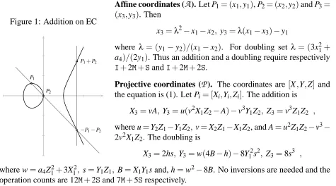
for the point[0,1,0]. The group law on these affine points is depicted in Figure 1. This rule is easily transformed into an explicit formula which manipulates the coordinates. To double a point P, we consider the tangent line to the curve at P instead of the secant.Figure 1: Addition on EC
P1
P2
−P1−P2 P1+P2
Affine coordinates (
A
). Let P1= (x1,y1), P2= (x2,y2)and P3= (x3,y3). Thenx3=λ2−x1−x2, y3=λ(x1−x3)−y1
where λ = (y1−y2)/(x1−x2). For doubling set λ = (3x21+
a4)/(2y1). Thus an addition and a doubling require respectively
I+2M+SandI+2M+2S.
Projective coordinates (
P
). The coordinates are [X,Y,Z] and the equation is (1). Let Pi= [Xi,Yi,Zi]. The addition isX3=vA, Y3=u(v2X1Z2−A)−v3Y1Z2, Z3=v3Z1Z2 ,
where u=Y2Z1−Y1Z2, v=X2Z1−X1Z2, and A=u2Z1Z2−v3− 2v2X1Z2. The doubling is
X3=2hs,Y3=w(4B−h)−8Y12s2, Z3=8s3 ,
where w=a4Z12+3X12, s=Y1Z1, B=X1Y1s and, h=w2−8B. No inversions are needed and the operation counts are 12M+2Sand 7M+5Srespectively.
Jacobian and Chudnovsky Jacobian coordinates (
J
andJ
c). In Jacobian coordinates theequa-tion of E is
where x=X/Z2 and y=Y/Z3. Let (Xi,Yi,Zi) be the coordinates of the point Pi. The addition
P3=P1+P2is given by
X3=−H3−2U1H2+r2,Y3=−S1H3+r(U1H2−X3), Z3=Z1Z2H ,
where U1=X1Z22,U2=X2Z12, S1=Y1Z23, S2=Y2Z13, H=U2−U1and r=S2−S1. The doubling is given by
X3=T, Y3=−8Y14+M(S−T), Z3=2Y1Z1 ,
where S=4X1Y12, M=3X12+a4Z14and T =−2S+M2. The operation counts are 12M+4S and 4M+6Srespectively.
For a point Pi, the quintuple (Xi,Yi,Zi,Zi2,Zi3) are the Chudnovsky (Jacobian) coordinates. The
same formulae as for
J
are used, and we do not have to compute Z12, Z22, Z13 and Z23, but we must compute Z32and Z33. The operation counts become 11M+3Sand 5M+6S.Modified Jacobian coordinates (
J
m). This set of coordinates was introduced by Cohen et al. [9].It is based on
J
but the internal representation of a point P is the quadruple(X,Y,Z,a4Z4). The formulae are almost the same as forJ
, the main difference being the introduction of U =8Y14so that Y3=M(S−T)−U and a4Z43=2U(a4Z14). An addition takes 13M+6Sand a doubling 4M+4S. SinceItakes on average between 9 and 40MandSis about 0.5Mto 0.8M, this system provides the fastest doubling in practice.Mixed Coordinate Systems. Different coordinate systems can be used together to perform scalar
multiplications. It is always advantageous to keep the base point and all precomputed points in
A
, since additions by those points will be less expensive. For the doublings one should choose the coordinate system which has the fastest doubling. More refined strategies are possible: see [9], where detailed operation counts for group operations with mixed coordinates are given. The same approach can be followed for genus 2 HEC (see Subsubsection 2.3.2.1 and Subsection 2.4).1.2
Hyperelliptic Jacobians
An excellent, low brow, introduction to hyperelliptic curves is given in [41], including proofs of the facts used below. Our notation is slightly different, but conform to that of [30, 31, 32, 33, 50].
1.2.1 Equation and Divisor Representation
A hyperelliptic curve
C
of genus g over a finite field Fq of odd characteristic is defined by a Weierstrass equationC
: y2= f(x) , (2)where f is a monic square-free polynomial of degree 2g+1 in x. Let ∞ be the point at infinity on the curve. In general, the points on a hyperelliptic curve do not form a group. Instead, the
A divisor D is a formal sum of points on the curve, considered with multiplicities, or, in other words, any element of the free Abelian groupZ[
C
(Fq)]. Its degree is the sum of those multiplici-ties, and its support the set of points with nonzero multiplicity. We are interested in the divisors of degree zero given by sums of the formm
∑
i=1
Pi−m∞ : Pi∈
C
r{∞} . (3)The degree of the associated effective divisor is the integer m. The points Piform the finite support
of D. The principal divisors are the divisors of functions, i. e. those whose points are the poles and zeros of a rational function on the curve, the multiplicity of each point being the order of the zero or minus the order of the pole at that point. The divisor class group is the quotient group of the degree zero divisors modulo the principal divisors. In each divisor class there exists a unique element of the form (3) with (effective) degree m≤g.
Figure 2: Addition on genus 2 HEC
P1
P2
Q1
Q2
−R1
−R2
R1
R2
(P1+P2−2∞) + (Q1+Q2−2∞) =
=R1+R2−2∞
To add two classes c1,c2 we formally add the rep-resenting divisors D1,D2. In general, this sum has degree >g, in which case it must be reduced to the
equivalent divisor of effective degree ≤g. To do
this, we consider a plane curve passing through the finite points of D1 and D2, counted with their mul-tiplicities – i. e. we determine a function f on the curve vanishing on the points on D1+D2, with mul-tiplicities taken into account, the only pole being at
∞. Put D3 the divisor whose (finite) support con-sists of the other points of intersection of the curve (with multiplicities). The class c3 of D3 satisfies
c1+c2+c3=0. It suffices to replace each point in
D3with its opposite (i.e. invert the y–coordinates) to get a divisor equivalent to D1+D2, but with smaller degree. We might have to repeat this step more than once to get the reduced element. This addition is depicted in Figure 2 for a genus 2 curve “geomet-rically”.
Mumford [47] introduced a representation of the elements of the divisor class group as polynomial pairs, for which Cantor [7] provided an explicit arithmetic algorithm. Let D=∑mi=1Pi−m∞be a
divisor with m≤g. The ideal class associated to D is represented by a unique pair of polynomials U(x),V(x)∈Fq[x]with g≥degU>degV , U monic and such that: U(x) =∏m
i=1(x−xPi)(i.e. the
roots of U(x) are the x–coordinates of the points belonging to the divisor); V(xPi) =yPi for all
1.2.2 Composition Algorithms
We consider the group operations on curves of arbitrary genus here. For explanations and proofs we refer the interested reader to [7]. The operation is split into two algorithms.
The first algorithm composes two divisors, and the result is in semi-reduced form: the output is a divisor D= [U,V]where the condition g≥degtU is not necessarily satisfied, but degtU >degtV .
This corresponds to the addition two divisors in the geometric way.
Algorithm 1: Divisor Composition
Input: D1= [U1,V1],D2= [U2,V2],
Output:D= [u,v]semi-reduced with D≡D1+D2.
1. compute d1,e1,e2 : d1=gcd(U1,U2) =e1U1+e2U2;
2. compute d,c1,c2 : d=gcd(d1,V1+V2) =c1d1+c2(V1+V2);
3. s1←c1e1, s2←c1e2, s3←c2; [i.e. d=s1U1+s2U2+s3(V1+V2)]
4. u←(U1U2)/(d2);
v←(s1U1V2+s2U2V1+s3(V1V2+f))/d mod U.
The second algorithm computes the Mumford representation of the unique representant of effective degree at most g in the divisor class of the input.
Algorithm 2: Divisor Reduction
Input: D= [U,V]semi-reduced.
Output:D0= [U0,V0]reduced with D≡D0.
1. U0←(f−V2)/U , V0← −V mod U0;
2. if degU0>g then put U←U0,V ←V0; goto 1;
3. make U0 monic.
1.2.3 Coordinate Systems
1.2.3.1 The general case
Let a reduced divisor D of a genus g curve be represented by two polynomials U(x),V(x)∈Fq[x] with g≥degU>degV , and U monic. In the most common case, write U(x) =xg+∑gi=−01Uixiand
1.2.3.2 Genus 2
For genus 2 there are two more coordinate systems besides affine (
A
).Miyamoto, Doi, Matsuo, Chao, and Tsuji [45] introduced projective coordinates (
P
): a quintu-ple[U1,U0,V1,V0,Z]corresponds to the divisor class represented by[t2+U1/Z t+U0/Z,V1/Z t+V0/Z]. Lange improved the operation counts of [45] and extended the work to even characteristic. To convert to the system
A
we needI+4M.Lange’s new coordinates [32] (
N
) are a weighted system, in the spirit of elliptic Jacobian co-ordinates: The sextuple [U1,U0,V1,V0,Z1,Z2] corresponds to the divisor class [t2+U1/Z12t+U0/Z12,V1/Z13Z2t+V0/Z13Z2]. The system
N
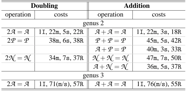
provides the fastest doubling, and is therefore impor-tant in scalar multiplications, where the doublings are the most common operation.The operation counts for the different operations are given in Table 4 on page 14. We do not list all the group operations here. Full details are given in [33].
2
Implementation
2.1
Prime Field Library
We already mentioned in the introduction that standard software libraries for performing arith-metic computations introduce several types of overheads. One is the fixed function call overhead. Other ones come from the fact they process operands of variable length in loops: They are usually negligible for very large operands, since the conditional branches in the loops in the code are most of the time taken for free. In fact, the branch prediction unit of the CPU will almost always guess the right branch, and the only misprediction shall occur when exiting the loop, i.e. the only time the branch is not taken. For operands of size relevant for curve cryptography the CPU will spend more time performing jumps and paying big penalties because of branch mispredictions than doing arithmetic. Thus, The smaller the field becomes, the higher will be the time wasted in the over-heads. Because of the larger number of field operations in smaller fields, HEC suffer from a much larger performance loss than EC.
multi-precision routines from the single word operations mentioned above. There are almost no conditional branches, so the CPU will seldom make very expensive branch mispredictions.
There are separate addition, subtraction, multiplication and modular inversion routines for all operand sizes, in steps of 32 bits from 32 to 256 bits, as well as for 48–bit fields (80 and 112-bit fields have been implemented too, but gave no speed advantage with respect to the 96 and 128-bit routines). All elements ofZ/NZare stored in vectors of the same length of 32-bit words. With the exception of 32-bit operands, inversion is based on the extended binary GCD, and uses an almost-inverse like algorithm [24, 57] with final multiplication from a table of precomputed, reduced, powers of 2. This is usually the fastest approach up to about 192 bits. For 32-bit operands better performance is attained with an implementation of the extended Euclidean algorithm with separate consideration of small quotients. Inversion was not sped up further for larger input sizes because of the intended usage of the library. In the case of elliptic curves, inversion-free coordinate systems are much faster than affine coordinates, so there is need, basically, only for one inversion at the end of a scalar multiplication. In the case of hyperelliptic curves, fields are quite small (32 to 128 bits in most cases) in which case our inversion routines have optimal performance anyway. Hence, Lehmer’s method or the recent improvements by Jebelean [22, 23] or Lercier [38] have not been included.
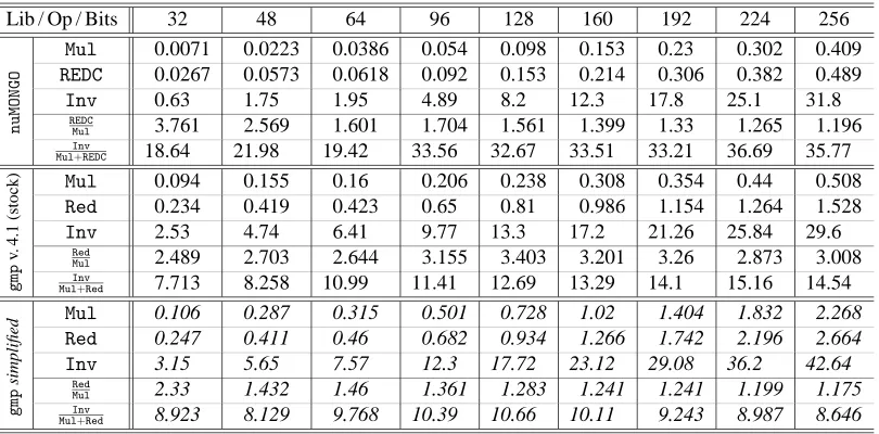
Table 1: Timings of basic operations in µsec (1 Ghz AMD Athlon PC) and ratios
Lib / Op / Bits 32 48 64 96 128 160 192 224 256
nuMONGO
Mul 0.0071 0.0223 0.0386 0.054 0.098 0.153 0.23 0.302 0.409 REDC 0.0267 0.0573 0.0618 0.092 0.153 0.214 0.306 0.382 0.489
Inv 0.63 1.75 1.95 4.89 8.2 12.3 17.8 25.1 31.8 REDC
Mul 3.761 2.569 1.601 1.704 1.561 1.399 1.33 1.265 1.196 Inv
Mul+REDC 18.64 21.98 19.42 33.56 32.67 33.51 33.21 36.69 35.77
gmp
v.
4.1
(stock)
Mul 0.094 0.155 0.16 0.206 0.238 0.308 0.354 0.44 0.508 Red 0.234 0.419 0.423 0.65 0.81 0.986 1.154 1.264 1.528 Inv 2.53 4.74 6.41 9.77 13.3 17.2 21.26 25.84 29.6
Red
Mul 2.489 2.703 2.644 3.155 3.403 3.201 3.26 2.873 3.008 Inv
Mul+Red 7.713 8.258 10.99 11.41 12.69 13.29 14.1 15.16 14.54
gmp
simplified
Mul 0.106 0.287 0.315 0.501 0.728 1.02 1.404 1.832 2.268 Red 0.247 0.411 0.46 0.682 0.934 1.266 1.742 2.196 2.664 Inv 3.15 5.65 7.57 12.3 17.72 23.12 29.08 36.2 42.64
Red
Mul 2.33 1.432 1.46 1.361 1.283 1.241 1.241 1.199 1.175 Inv
Mul+Red 8.923 8.129 9.768 10.39 10.66 10.11 9.243 8.987 8.646
In Table 1 we show some timings of basic operations with gmp version 4.1 and nuMONGO. The timings have been measured on a PC with a 1 Ghz AMD Athlon Model 4 processor, as all other timings in this paper, under the Linux operating system (kernel version 2.4.18). Our programs have been compiled with the GNU Compiler Collection (gcc) version 2.95.3. We now describe the meaning of the table entries.
and RedMul) and of an inversion to the time of a multiplication together with a reduction (MulInv+REDC and
Inv
Mul+Red) are given: The first ratio tells how many “multiplications” we save each time we save a
reduction using the techniques described in the next subsection; the second ratio is the cost of a field inversion in multiplications. The columns correspond to the bit lengths of the operands. Note thatgmpis very heavily optimized in assembler for the considered architecture, whereas the inner loops of nuMONGOare far less optimized. The timings corresponding to this stock, highly optimized version of gmpare given in the group labeledgmpversion 4.1 (stock). It is possible to recompilegmpusing only C with some assembler macros, i.e. the same type of approach used for
nuMONGO, thus losing performance: This fact has been observed also in [5] in a slightly different contexts. The corresponding timings are given in the group labeledgmpsimplified.
A few remarks:
(1) nuMONGOcan perform better than a far more optimized, but general purpose library.
(2) The disparity with a general purpose library compiled with the same optimization level as
nuMONGOis considerable.
(3) For larger operands gmp catches up with nuMONGO, the modular reduction remaining slower because it is not based on Montgomery’s algorithm.
(4) nuMONGOhas the highest ratio of a field inversion to a field multiplication. This shows how big the overheads in general purpose libraries are for such small inputs. In particular, such ratios are quite close to those in hardware implementation of field arithmetic.
2.2
Lazy and Incomplete reduction
Lazy and incomplete modular reduction are described in [5]. Here, we give a short treatment. Let
p be a prime number smaller than 2w, where w is a fixed integer. We consider the evaluation of expressions of the form ∑di=−01aibi mod p given ai and bi with 0≤ai,bi < p. Such expressions
occur in polynomial multiplication, hence in the explicit formulae for HEC.
To use most modular reduction algorithms or Montgomery’s reduction procedure [46] at the end of the summation, we have to make sure that all partial sums of ∑aibi are smaller than p 2w.
Some authors (see for example [39]) suggested to use small primes, to guarantee that the condition
∑aibi < p 2w is always satisfied in a given situation. However, doing this would contradict the
main design principle ofnuMONGO, which is to have no restriction on p except that it must fit in the available number of machine words allocated for it.
What we do instead is to ensure that the number obtained by removing the least significant w bits of any intermediate result remains < p. We do this by adding the products aibi in succession,
and checking if there has been an overflow or if the most significant half of the intermediate sum is≥ p : if so we subtract p from the number obtained ignoring the w least significant bits of the
intermediate result. If the intermediate result is≥22w, the additional bit can be stored in a carry. Since all intermediate results are bounded by p22w+1<(p+2w)2w, upon subtraction of p 2w the
and at the end we have to reduce a number bounded by p 2w, making the modular reduction easier and possibly faster.
Algorithm 3: Incomplete reduction
Input: p<2w, aiand bi<p for i=0, . . . ,t,
Output: x with x≡∑ti=0aibi mod p2wand 0≤x≤p2w Notation:x=xhi·2w+xlo where xhi,xlo<2w
1. Initialise x←a0b0 for i=1 to t do {
2. carry·22w+x←x+aibi (with x<22wandcarry∈ {0,1})
3. if carry or xhi≥p then xhi←xhi−p mod 2w}
4. returnx
We implemented some APIs innuMONGO for supporting Lazy (i.e. delayed) and Incomplete (i.e. limited to the most significant half of the considered operands) modular reduction. They can also be used in the implementation of the arithmetic of extension fields.
nuMONGOsupports Lazy (i.e. delayed) and Incomplete (i.e. limited to the number obtained by re-moving the least significant w bits) modular reduction. Thus, an expression of the form ∑di=−01aibi
mod p can be evaluated by d multiplications but only one modular reduction instead of d. A modular reduction is at least as expensive as a multiplication, and often much more, see Table 1. Registers which can hold values up to 2w−1 are called short registers, those who can hold values up to 22w−1 are called wide registers.
Remark 2.1. We cannot add a reduced element to an unreduced element in Montgomery’s repre-sentation. This is due to the fact that Montgomery’s representation ˆa of the integer a is aR mod p, where R is a power of 2 larger than p. Now, ˆa ˆb is congruent to abR2modulo p, not tocab. Therefore, adding a number in Montgomery’s representation to ˆa ˆb would give meaningless results.
For most small values of w, all above operations are inlined, so the code size of the second imple-mentation will be actually smaller than in the first impleimple-mentation, due to the reduced number of modular reductions. This makes it even more likely that the code implementing group operations will fit entirely in the CPU’s level 1 cache. For large w (w≤192) the operatorsAdd,Sub,Mul, etc. are never inlined to keep the code of the whole group operations in the level 1 cache of the target CPU.
2.3
Implementation of the Explicit Formulae
2.3.1 Elliptic Curves
For EC, only few savings inREDCs are possible by using lazy and incomplete reduction.
Table 2: Costs of Group Operations on EC, with lazy reduction
Doubling Addition
operation costs operation costs operation costs
2A=A I, 2m, 2s, 4R A+A=A I, 2m, 1s, 3R
2P =P 7m, 5s, 10R P+P =P 12m, 2s, 13R A+P =P 9m, 2s, 10R
2J =J 4m, 6s, 8R J+J =J 12m, 4s, 16R A+J =J 8m, 3s, 11R
2Jc=Jc 5m, 6s, 9R Jc+Jc=Jc 11m, 3s, 14R A+Jc=Jc 8m, 3s, 11R
2Jm=Jm 4m, 4s, 8R Jm+Jm=Jm 13m, 6s, 19R A+Jm=Jm 9m, 5s, 14R
P3 = [X3,Y3,Z3]. The addition P3 =P1+P2 is done by performing the following operations in order [9]:
u=Y2−Y1Z2 v=X2−X1Z2, A=u2Z2−v3−2v2X1Z2,
X3=vA, Y3=u(v2X1Z2−A)−v3Y1Z2, Z3=v3Z2 .
For the computation of u and v no savings are possible. Consider the expression A=u2Z2−v3− 2v2X1Z2. We could hope to save reductions in its computation, but: We need v3 reduced anyway for Z3, A must be available also in reduced form to compute X3, and from v2X1Z2we subtract A in the computation of Y3. It is easy that here no gain is obtained by delaying reduction. But Y3 can be computed by first multiplying without reducing u by v2X1Z2−A, then v3by Y1Z2, adding these two products and reducing the sum. Hence, in the addition formula oneREDCcan be saved. For affine coordinates, no REDCs can be saved. Additions in
P
allow saving of 1 REDC, even if one of the two points is inA
. With no other addition formula we can save reductions. For all doublings we can save 2REDCs, except for the doubling inJ
m, where no savings can be done due to the differences in the formulae depending on the introduction of a4Z4. In Table 2, we write the operation counts of the operations which we implemented. The number of REDCs is given separately from the multiplications and squarings.2.3.2 Hyperelliptic Curves
To derive explicit formulae, one starts with Cantor’s algorithm and “unrolls” the steps in order. First, one must consider which cases can occur, which depend on the degrees of the input divisors and, in the case of the addition, whether the supports of the two divisors to be added contain points with the same x–coordinates. The cases that almost always occur (with probability 1−
In the next subsubsections, we analyse the extent of applicability of lazy and incomplete reduction in the formulae for the types of curves which we consider.
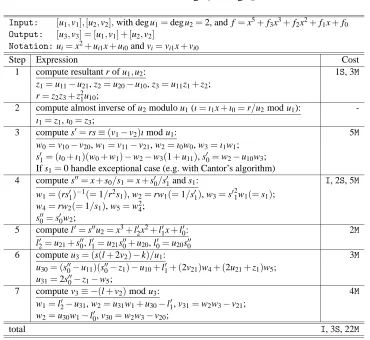
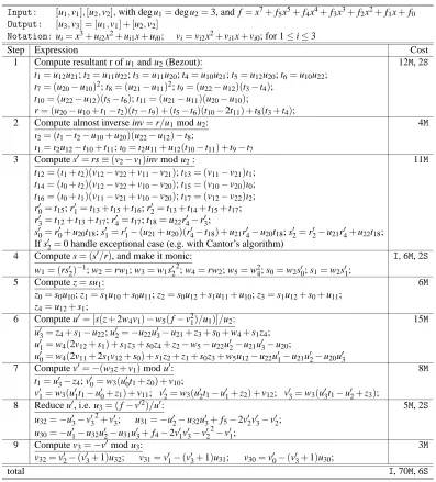
2.3.2.1 Genus 2 We now see in a concrete case – namely a particular genus 2 formula – how wide operations are used in practice. Table 3 is derived from results in [30], but restricted to the odd characteristic case. Also we do not distinguish between squarings and multiplications. The
Table 3: Addition, deg u1=deg u2=2
Input: [u1,v1],[u2,v2],with deg u1=deg u2=2, and f =x5+f3x3+f2x2+f1x+f0 Output: [u3,v3] = [u1,v1] + [u2,v2]
Notation:ui=x2+ui1x+ui0and vi=vi1x+vi0
Step Expression Cost
1 compute resultant r of u1,u2: 1S, 3M
z1=u11−u21, z2=u20−u10, z3=u11z1+z2; r=z2z3+z21u10;
2 compute almost inverse of u2modulo u1(ı=ı1x+ı0=r/u2mod u1): -ı1=z1, ı0=z3;
3 compute s0=rs≡(v1−v2)ı mod u1: 5M w0=v10−v20, w1=v11−v21, w2=ı0w0, w3=ı1w1;
s01= (ı0+ı1)(w0+w1)−w2−w3(1+u11), s00 =w2−u10w3; If s1=0 handle exceptional case (e.g. with Cantor’s algorithm)
4 compute s00=x+s0/s1=x+s00/s01and s1: I, 2S, 5M w1= (rs01)−
1(=1/r2s
1), w2=rw1(=1/s01), w3=s021w1(=s1); w4=rw2(=1/s1), w5=w24;
s000=s00w2;
5 compute l0=s00u2=x3+l20x2+l10x+l00: 2M l20=u21+s000, l10=u21s000+u20, l00=u20s000
6 compute u3= (s(l+2v2)−k)/u1: 3M u30= (s000−u11)(s000−z1)−u10+l10+ (2v21)w4+ (2u21+z1)w5;
u31=2s000−z1−w5;
7 compute v3≡ −(l+v2)mod u3: 4M
w1=l02−u31, w2=u31w1+u30−l10, v31=w2w3−v21; w2=u30w1−l00, v30=w2w3−v20;
total I, 3S, 22M
detailed breakdown of the reductions saved due to the use of wide operands follows:
1. In Step 1 we can save oneREDCin the computation of r, since we do not need the reduced value of z2z3and z21u10 anywhere else.
2. In Step 3 we do not reduce w2=ı0w0, since it is used in the computation of s01and s00, which are sums of products of two elements. So only 3 REDCs are required to implement Step 3: for w3and for the final results of s01and s00. This is a saving of twoREDCs.
Table 4: Costs of Group Operations for HEC, with lazy reduction
Doubling Addition
operation costs operation costs
genus 2
2A=A 1I, 22m, 5s, 22R A+A =A 1I, 22m, 3s, 18R 2P=P 38m, 6s, 38R P+P=P 45m, 5s, 42R A+P =P 40m, 3s, 33R 2N =N 34m, 7s, 37R N +N =N 47m, 7s, 50R A+N =N 36m, 5s, 37R genus 3
2A=A 1I, 71(m/s), 57R A+A =A 1I, 76(m/s), 55R
But l10 =u21s000+u20is a problem: we cannot add reduced and unreduced quantities (see Re-mark 2.1). We circumvent this by computing the unreduced products L1=u21s000(in place of
`01) and L0=u20s000. TwoREDCs are saved.
4. In Step 6, it is u00= (s000−u11)(s000−z1) +L1+2v21w4+ (2u21+z1)w5+z2. We need only oneREDC to compute the (reduced) sum of the first four products: Note that, at this point,
L1is already known and we already counted the saving of oneREDCassociated to it. So, we save a total of twoREDCs.
Summarizing, to implement addition for genus 2 curves in affine coordinates in the most common case, we need 12Muls, 13MulNoREDCs and 6REDCs. Thus, we save 7REDCs.
We implemented addition and doubling in all coordinate systems. In order to speed-up scalar multiplication, we also implemented addition in the cases where one of the two points to be added is given in
A
and the other one inP
orN
, with result inP
orN
respectively.In Table 4 we show the operation counts of the operations implemented, counting separately the number ofREDCs.
The table contains also the counts for the genus 3 case (see the next Subsubsection). One sees at once that the number of modular reductions is always significantly smaller than the total number of multiplications.
report the correct formulae for addition and doubling in genus 3 in odd characteristic and on curves of equation y2= f(x), where the second most significant coefficient of f vanishes.
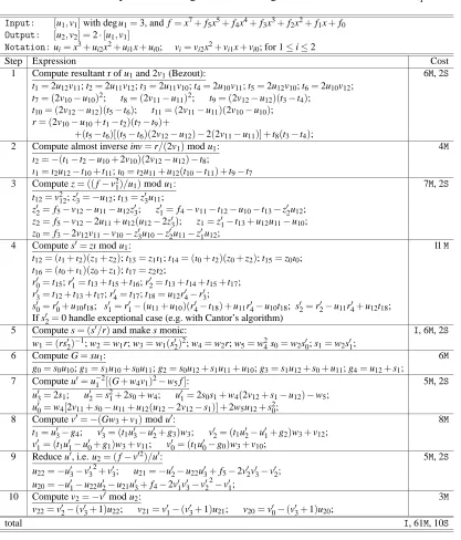
Table 5: Explicit addition formula on a genus three Jacobian overFq
Input: [u1,v1],[u2,v2],with deg u1=deg u2=3, and f=x7+f5x5+f4x4+f3x3+f2x2+f1x+f0
Output: [u3,v3] = [u1,v1] + [u2,v2]
Notation:ui=x3+ui2x2+ui1x+ui0; vi=vi2x2+vi1x+vi0; for 1≤i≤3
Step Expression Cost
1 Compute resultant r of u1and u2(Bezout): 12M, 2S
t1=u12u21; t2=u11u22; t3=u11u20; t4=u10u21; t5=u12u20; t6=u10u22;
t7= (u20−u10)2; t8= (u21−u11)2; t9= (u22−u12)(t3−t4);
t10= (u22−u12)(t5−t6); t11= (u21−u11)(u20−u10);
r= (u20−u10+t1−t2)(t7−t9) + (t5−t6)(t10−2t11) +t8(t3+t4);
2 Compute almost inverse inv=r/u1mod u2: 4M
ı2= (t1−t2−u10+u20)(u22−u12)−t8;
ı1=ı2u12−t10+t11; ı0=ı2u11+u12(t10−t11) +t9−t7
3 Compute s0=rs≡(v2−v1)inv mod u2: 11M
t12= (ı1+ı2)(v12−v22+v11−v21); t13= (v11−v21)ı1;
t14= (ı0+ı2)(v12−v22+v10−v20); t15= (v10−v20)ı0;
t16= (ı0+ı1)(v11−v21+v10−v20); t17= (v12−v22)ı2;
r00=t15; r10=t13+t15+t16; r02=t13+t14+t15+t17;
r30=t12+t13+t17; r40=t17; t18=u22r40−r30;
s00=r00+u20t18; s01=r10−(u21+u20)(r04−t18) +u21r04−u20t18; s02=r02−u21r04+u22t18;
If s02=0 handle exceptional case (e.g. with Cantor’s algorithm)
4 Compute s= (s0/r), and make it monic: I, 6M, 2S
w1= (rs02)−1; w2=rw1; w3=w1s02 2
; w4=rw2; w5=w24; s0=w2s00; s1=w2s01;
5 Compute z=su1: 6M
z0=s0u10; z1=s1u10+s0u11; z2=s0u12+s1u11+u10; z3=s1u12+s0+u11;
z4=u12+s1;
6 Compute u0= [s(z+2w4v1)−w5(f−v21)/u1)]/u2: 15M
u03=z4+s1−u22; u02=−u22u03−u21+z3+s0+w4+s1z4;
u01=w4(2v12+s1) +s1z3+s0z4+z2−w5−u22u20−u21u03−u20;
u00=w4(2v11+2s1v12+s0) +s1z2+z1+s0z3+w5u12−u22u10−u21u02−u20u03
7 Compute v0=−(w3z+v1)mod u0: 8M
t1=u03−z4; v00=w3(u00t1+z0) +v10;
v01=w3(u01t1−u00+z1) +v11; v02=w3(u02t1−u01+z2) +v12; v03=w3(u03t1−u02+z3);
8 Reduce u0, i.e. u3= (f−v02)/u0: 5M, 2S
u32=−u03−v03 2
+v03; u31=−u02−u32u03+f5−2v02v03−v02;
u30=−u01−u32u02−u31u03+f4−2v01v03−v02 2
−v01;
9 Compute v3=−v0mod u3: 3M
v32=v02−(v03+1)u32; v31=v01−(v03+1)u31; v30=v00−(v03+1)u30;
total I, 70M, 6S
A pleasant aspect of the genus three formulae is that a large proportion of modular reductions can be saved: at least 21 in the addition and 14 in the doubling (see Table 4 on the preceding page).
2.4
Scalar Multiplication
Table 6: Explicit doubling formula on a genus three Jacobian overFq
Input: [u1,v1]with deg u1=3, and f=x7+f5x5+f4x4+f3x3+f2x2+f1x+f0
Output: [u2,v2] =2·[u1,v1]
Notation:ui=x3+ui2x2+ui1x+ui0; vi=vi2x2+vi1x+vi0; for 1≤i≤2
Step Expression Cost
1 Compute resultant r of u1and 2v1(Bezout): 6M, 2S
t1=2u12v11; t2=2u11v12; t3=2u11v10; t4=2u10v11; t5=2u12v10; t6=2u10v12;
t7= (2v10−u10)2; t8= (2v11−u11)2; t9= (2v12−u12)(t3−t4);
t10= (2v12−u12)(t5−t6); t11= (2v11−u11)(2v10−u10);
r= (2v10−u10+t1−t2)(t7−t9)+
+(t5−t6)[(t5−t6)(2v12−u12)−2(2v11−u11)] +t8(t3−t4);
2 Compute almost inverse inv=r/(2v1)mod u1: 4M
ı2=−(t1−t2−u10+2v10)(2v12−u12)−t8;
ı1=ı2u12−t10+t11; ı0=ı2u11+u12(t10−t11) +t9−t7
3 Compute z= ((f−v21)/u1)mod u1: 7M, 2S
t12=v212; z03=−u12; t13=z03u11;
z02=f5−v12−u11−u12z03; z01= f4−v11−t12−u10−t13−z02u12;
z2=f5−v12−2u11+u12(u12−2z30); z1=z01−t13+u12u11−u10;
z0=f3−2v12v11−v10−z30u10−z02u11−z01u12;
4 Compute s0=zı mod u1: 11M
t12= (ı1+ı2)(z1+z2); t13=z1ı1; t14= (ı0+ı2)(z0+z2); t15=z0ı0;
t16= (ı0+ı1)(z0+z1); t17=z2ı2;
r00=t15; r10=t13+t15+t16; r20=t13+t14+t15+t17;
r03=t12+t13+t17; r04=t17; t18=u12r04−r03;
s00=r00+u10t18; s01=r01−(u11+u10)(r40−t18) +u11r40−u10t18; s02=r20−u11r04+u12t18;
If s02=0 handle exceptional case (e.g. with Cantor’s algorithm)
5 Compute s= (s0/r)and make s monic: I, 6M, 2S
w1= (rs02)−1; w2=w1r; w3=w1(s02)2; w4=w2r; w5=w24s0=w2s00; s1=w2s01;
6 Compute G=su1: 6M
g0=s0u10; g1=s1u10+s0u11; g2=s0u12+s1u11+u10; g3=s1u12+s0+u11; g4=u12+s1;
7 Compute u0=u−12[(G+w4v1)2−w5f]: 5M, 2S
u03=2s1; u02=s21+2s0+w4; u10=2s0s1+w4(2v12+s1−u12)−w5;
u00=w4[2v11+s0−u11+u12(u12−2v12−s1)] +2w5u12+s20;
8 Compute v0=−(Gw3+v1)mod u0: 8M
t1=u03−g4; v03= (t1u03−u02+g3)w3; v02= (t1u02−u01+g2)w3+v12;
v01= (t1u01−u00+g1)w3+v11; v00= (t1u00−g0)w3+v10;
9 Reduce u0, i.e. u2= (f−v02)/u0: 5M, 2S
u22=−u03−v03 2+
v03; u21=−u02−u22u30+f5−2v02v03−v02;
u20=−u01−u22u02−u21u03+f4−2v01v03−v02 2
−v01;
10 Compute v2=−v0mod u2: 3M
v22=v02−(v03+1)u22; v21=v01−(v03+1)u21; v20=v00−(v03+1)u20;
total I, 61M, 10S
A simple method for computing s·D for an integer s and a divisor D is based on the binary
representation of s. If s=∑ni=−01si2iwhere each si=0 or 1, then n·D can be computed as
sD=2(2(···2(2(sn−1D) +sn−2D) +···) +s1D) +s0D. (4) This requires n−1 doublings and on average n/2 additions on the curve.
to a method needing n doublings and on average n/3 additions or subtractions.
A generalization of the NAF comes from using “sliding windows”. The wNAF [60, 8] of the integer
s is a representation s=∑nj=0sj2jwhere the integers sjsatisfy the following two conditions: (i)
ei-ther sj=0 or sjis odd and|sj| ≤2w; (ii) of any w+1 consecutive coefficients sj+w, . . . ,sjat most
one is nonzero.
The 1NAF coincides with the NAF. The wNAF has average density 1/(w+2). To compute a scalar multiplication based on the wNAF one must first precompute the divisors D, 3D, . . . ,(2w−1)D,
and then perform a double-and-add step like (4).
3
Results and Comparisons
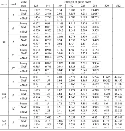
Table 7 on page 20 reports the timings of our implementation. Since nuMONGOprovides support only for moduli up to 256 bits, EC are tested only on fields up to that size. For genus 2 curves on a 256 bit field, a group up to 512 bits is possible: We choose this group size as a limit also for our tests of genus 3 curves.
All benchmarks were performed on a 1 Ghz AMD Athlon (Model 4) PC, under the Linux operating system (kernel version 2.4.18). The compiler used was the GNU Compiler Collection (gcc) version 2.95.3. The elliptic curves all have almost prime order and have been found by point counting on random curves. The genus 2 and 3 curves have rational divisor class groups of almost prime order and have been costructed by complex multiplication.
For each combination of group type (EC and HEC of genus 2 and 3), coordinate system and bit size of the group (not of the field!), we averaged the timings of several thousands scalar multiplications with random scalars, and performed the scalar multiplication using three different recodings of the scalar: the binary representation, the NAF, and the wNAF. For the wNAF we report only the best timing and the value of w for which it is attained. When using the various coordinate systems, we always keep the base divisor and its multiples in affine coordinates, since adding an affine point to a point in any coordinate system is faster than adding two points in that coordinate system. In the timings for the wNAF the timings for the precomputations are always included in the results. For comparison with our timings, Lange [30] reported timings of 8.232 and 9.121 milliseconds for genus 2 curves with group order≈ 2160 and 2180 respectively on agmp-based implementation of affine coordinates on a Pentium IV processor running at 1.5 Ghz, and for antl-based the timings are 11.326 and 16.324 for the two curves above. The scalar multiplication in [30] is based on the double-and-add algorithm based on the unsigned binary representation. In [53], a timing of 98 milliseconds for a genus 3 curve of about 180 bits (p≈260) on an Alpha 21164A CPU running at 600MHz is reported. The speed of these two CPUs is close to that of the machine we used for our tests.
In Table 8 on page 21 we provide timings foreccandhecusinggmp(with the highest optimization possible) and the double-and-add scalar multiplication is based on the unsigned binary representa-tion. In Table 9 on page 21 we show the timings of thenuMONGOgenus 2 and 3hecimplementation without lazy and incomplete reduction.
(1) Using a specialised software library one can get a speed-up by a factor of 3 to 4.5 for EC with respect to a traditional implementation. The speed-up for genus 2 and 3 curves is up to 8.
(2) Lazy and incomplete modular reduction alone brings a speed-up from 3% to 7%.
(a) The speed-up is larger for genus 3 curves because a larger proportion of reductions is saved.
(b) For genus 2, the amount of modular reductions saved with new coordinates is smaller than with projective coordinates. As a result, the performance difference between the two coordinate systems is smaller than without lazy and incomplete reduction (for example, for 256-bit curves, the gain is 5.3% instead of 9.7%). It would be interesting to rewrite the explicit formulae for
N
to allow more savings in reduction.(3) HEC over prime fields are still slower than EC, but the gap has been narrowed.
(a) Affine coordinates for genus 2 HEC are significantly faster than those for EC. Those for genus 3 are faster from 144 bits upwards.
(b) Comparing the best coordinate systems and scalar multiplication algorithms for genus 2 HEC and EC, we see that:
(i) For 192 bit, resp. 256 bit curves, HEC is slower than EC by only 17%, resp. 12%. (ii) For other group sizes the difference is often around 50%.
(c) Genus 3 curves are slower than genus 2 ones. Whereas withgmpthe difference is 80% to 100% for 160 to 512 bit groups, usingnuMONGOthe difference is often as small as 50%.
(4) Using nuMONGOwe can successfully eliminate most of the overheads associated to function calls and to the processing of short operands. This proves the soundness of our approach.
(a) In thegmp-based implementation (see Table 8) the timings with different coordinate sys-tems are closer to each other than with nuMONGObecause of the big amount of time lost in the overheads. For HEC we even have the paradoxical result that
P
andN
are slower thanA
, because of they require significantly more function calls for each group operation thanA
. Therefore, withgmpin some cases the overheads dominate the running time. (b) For affine coordinates the dominant part of the operation is the field inversion, hence thespeed-up given by nuMONGOis not big, and is close to that in Table 1 on page 9 for the inversion alone. For the other coordinate systems, the speed-up becomes significant.
(5) If the field size for a given group is not close to a multiple of the machine word size, there is a relative drop in performance with respect to other groups where the field size is nicer.
(b) A similar phenomenon occurs when comparing 224-bit EC and genus 2 HEC groups. The performance loss of HEC is about 50%, due to the 112-bit field arithmetic, which is not a multiple of the native word size of the CPU. However, 192 bit and 256 bit HEC perform much better in comparison with EC.
We conclude that the performance of hyperelliptic curves over prime fields is satisfactory enough to be considered as a valid alternative to elliptic curves, especially when large point groups are desired, and the bit length of the characteristic is close to (but smaller than) a multiple of the machine word length.
In software implementations we should employ a custom software library, and for a further, non negligible, speed-up, use lazy and incomplete reduction.
References
[1] L. Adleman and J. DeMarrais. A subexponential algorithm for discrete logarithms over all finite fields, Mathe-matics of Computation, 61 (1993), pp. 1–15.
[2] L. Adleman, J. DeMarrais and M. Huang. A subexponential algorithm for discrete logarithms over the rational subgroup of the Jacobians of large genus hyperelliptic curves over finite fields. Algorithmic Number Theory, LNCS 877, pp. 28-40. Springer, 1994.
[3] R.M. Avanzi. Countermeasures against differential power analysis for hyperelliptic curve cryptosystems. In: Proceedings of CHES 2003, Cologne, Germany. LNCS 2779, pp. 366–381. Springer, 2003.
[4] R.M. Avanzi.nuMONGOand Description and Use of thenuMONGOLibrary. A software library and related docu-mentation. Available from the author.
[5] R.M. Avanzi and P.M. Mih˘ailescu. Generic Efficient Arithmetic Algorithms for PAFFs (Processor Adequate Finite Fields) and Related Algebraic Structures. To appear in proceedings of: Selected Areas in Cryptography 2003, Ottawa, August 14–15, 2003.
[6] M. Bauer. A subexponential algorithm for solving the discrete logarithm problem in the Jacobian of high genus hyperelliptic curves over arbitrary finite fields. Preprint, 1999.
[7] D. Cantor. Computing in the Jacobian of a Hyperelliptic Curve. Mathematics of Computation, 48 (1987), pp. 95– 101.
[8] H. Cohen, A. Miyaji and T. Ono. Efficient elliptic curve exponentiation. In Proceedings ICICS’97, LNCS 1334, pp. 282–290. Springer, 1997.
[9] H. Cohen, A. Miyaji and T. Ono. Efficient Elliptic Curve Exponentiation Using Mixed Coordinates, In: ASI-ACRYPT: Advances in Cryptology. LNCS 1514, pp. 51–65. Springer, 1998.
[10] D. Coppersmith. Fast evaluation of logarithms in fields of characteristic two. IEEE Transactions on Information Theory, 30 (1984), pp. 587–594.
[11] A. Enge and P. Gaudry. A general framework for subexponential discrete logarithm algorithms. Acta Arithmetica 102, pp. 83–103, 2002.
[12] M. Fouquet, P. Gaudry, and R. Harley. On Satoh’s algorithm and its implementation. Lix/RR/00/06, 2000. Preprint.
[13] P. Gaudry, An algorithm for solving the discrete log problem on hyperelliptic curves. In Proceedings of: Euro-crypt 2000, pp. 19–34. Springer LNCS, 2000.
[14] P. Gaudry and R. Harley. Counting points on hyperelliptic curves over finite fields. Proceedings of: ANTS-IV. LNCS 1838, pp. 313–332. Springer–Verlag, 2000.
[15] P. Gaudry and E. Schost. Cardinality of a genus 2 hyperelliptic curve over GF(5·1024+41). Email message to
Table 7: Comparison of running times, in msec (1 Ghz AMD Athlon PC)
scalar Bitlength of group order
curve coord.
mult. 128 144 160 192 224 256 320 512
binary 1.792 2.784 3.34 5.783 9.27 13.419
A NAF 1.575 2.466 2.98 5.153 8.211 12.087
wNAF 1.454(w 2.272 2.704 4.685 7.389 10.755 =3) (w=3) (w=4) (w=4) (w=4) (w=4) binary 0.672 0.98 1.168 1.915 2.826 4.295
P NAF 0.599 0.88 1.105 1.717 2.528 3.836
wNAF 0.579 0.852 1.012 1.643 2.509 3.558 (w=3) (w=3) (w=3) (w=3) (w=4) (w=3) binary 0.603 0.884 1.056 1.775 2.539 3.897
ec J NAF 0.541 0.792 0.94 1.532 2.242 3.479
wNAF 0.507(w 0.75 0.92 1.43 2.11 3.161 =3) (w=3) (w=2) (w=3) (w=3) (w=3) binary 0.632 0.946 1.132 1.88 2.734 4.154
Jc NAF 0.67 0.846 0.996 1.63 2.375 3.658
wNAF 0.541 0.804 0.972 1.523 2.281 3.431 (w=2) (w=3) (w=3) (w=3) (w=4) (w=3) binary 0.608 0.892 1.076 1.787 2.621 3.936
Jm NAF 0.515 0.768 0.914 1.525 2.22 3.399
wNAF 0.489(w 0.7 0.849 1.383 2.045 3.089 =3) (w=3) (w=3) (w=3) (w=3) (w=4)
binary 0.99 1.78 2.08 2.671 4.884 5.776 11.675 42.463
A NAF 0.907 1.57 1.94 2.399 4.365 5.205 10.325 38.457
wNAF 0.82 1.44 1.72 2.162 3.92 4.662 9.27 33.709
(w=3) (w=4) (w=4) (w=4) (w=4) (w=4) (w=5) (w=5) binary 1.073 1.55 1.82 2.174 4.095 4.718 9.225 31.928
hec P NAF 0.966 1.37 1.62 1.945 3.677 4.245 8.275 28.219
g=2 wNAF 0.906 1.29 1.533 1.766 3.339 3.848 7.37 25.104
(w=3) (w=4) (w=4) (w=4) (w=4) (w=4) (w=4) (w=5) binary 1.051 1.5 1.72 2.075 3.891 4.432 8.6 29.981
N NAF 0.946 1.3 1.51 1.846 3.447 3.945 7.25 26.468
wNAF 0.867 1.21 1.41 1.667 3.085 3.521 6.85 23.323 (w=3) (w=4) (w=4) (w=4) (w=4) (w=4) (w=4) (w=5) binary 2.332 2.612 4.7 5.653 5.67 6.82 13.22 47.843
hec A NAF 1.936 2.16 3.807 4.577 5.06 6.008 11.72 42.348
g=3 wNAF 1.604 1.808 2.792 3.538 4.53 5.343 10.28 36.209
(w=4) (w=4) (w=5) (w=5) (w=5) (w=5) (w=5) (w=5)
[16] P. Gaudry and E. Schost. Construction of Secure Random Curves of Genus 2 over Prime Fields. Submitted.
[17] R. Gerkmann. The p-adic Cohomology of Varieties over Finite Fields and Applications on the Computation of Zeta Functions. Ph.D. Thesis, University Duisburg-Essen, Campus Essen, 2003.
[18] D.M. Gordon. A survey of fast exponentiation methods. Journal of Algorithms 27, pp. 129–146, 1998.
[19] D. Gordon. Discrete logarithms in GF(p) using the number field sieve, SIAM Journal on Discrete Mathematics, 6 (1993), pp. 124–138.
Table 8: Timings withgmp, in msec (1 Ghz AMD Athlon PC)
ec 160 192 256
A 5.468 8.305 15.354
P 4.306 5.845 9.16
J 3.775 5.4 8.878
Jc 4.029 5.75 9.67
Jm 3.75 5.182 9.075
hec 160 192 256 320 512
A 9.292 12.082 18.873 29.5 72.09 g=2 P 12.15 14.961 23.442 32.212 81.586
N 11.349 13.278 20.4 28.93 74.389 g=3 A 19.799 22.452 40.39 59.691 129.541
Table 9: Timings withnuMONGOwithout lazy and incomplete reduction, in msec (1 Ghz AMD Athlon PC)
ec 160 192 256
A 3.396 5.946 13.638
P 1.224 2.094 4.592
J 1.12 1.897 4.095
Jc 1.182 2.001 4.354
Jm 1.096 1.816 4.036
hec 160 192 256 320 512
A 2.22 2.88 6.253 11.832 44.596 g=2 P 1.967 2.393 4.93 9.625 33.915
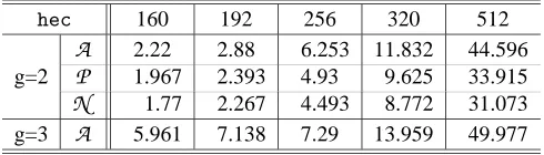
N 1.77 2.267 4.493 8.772 31.073 g=3 A 5.961 7.138 7.29 13.959 49.977
[21] R. Harley. Fast Arithmetic on Genus Two Curves.
Available athttp://cristal.inria.fr/~harley/hyper/
[22] T. Jebelean. A Generalization of the Binary GCD Algorithm. ISSAC 1993: pp. 111–116.
[23] T. Jebelean. A Double-Digit Lehmer-Euclid Algorithm for Finding the GCD of Long Integers. Journal of Sym-bolic Computation 19(1-3), pp. 145–157 (1995)
[24] B.S. Kaliski Jr.. The Montgomery inverse and its applications. IEEE Transactions on Computers, 44(8), pp. 1064–1065, August 1995.
[25] K.S. Kedlaya. Counting Points on Hyperelliptic Curves using Monsky-Washnitzer Cohomology. Journal of the Ramanujan Mathematical Society 16, pp. 323–338, 2001.
[26] N. Koblitz. Hyperelliptic Cryptosystems. Journal of Cryptology 1, pp. 139–150, 1989.
[27] N. Koblitz. Algebraic aspects of cryptography. Springer, 1998.
[28] U. Krieger. signature.c:Anwendung hyperelliptischer Kurven in der Kryptographie. M.S. Thesis, Mathe-matik und InforMathe-matik, Universit¨at Essen, Fachbereich 6, Essen, Germany.
[29] J. Kuroki, M. Gonda, K. Matsuo, J. Chao and S. Tsujii. Fast Genus Three Hyperelliptic Curve Cryptosystems. In: The 2002 Symposium on Cryptography and Information Security, Japan - SCIS 2002, Jan. 29–Feb. 1 2002.
[30] T. Lange. Efficient Arithmetic on Genus 2 Hyperelliptic Curves over Finite Fields via Explicit Formulae. Cryp-tology ePrint Archive, Report 2002/121, 2002.http://eprint.iacr.org/
[31] T. Lange. Inversion-Free Arithmetic on Genus 2 Hyperelliptic Curves. Cryptology ePrint Archive, Report 2002/147, 2002.http://eprint.iacr.org/
[32] T. Lange. Weighted Coordinates on Genus 2 Hyperelliptic Curves. Cryptology ePrint Archive, Report 2002/153, 2002.http://eprint.iacr.org/
[33] T. Lange. Formulae for Arithmetic on Genus 2 Hyperelliptic Curves. Preprint. Available from:http://www.ruhr-uni-bochum.de/itsc/tanja/
[34] A. Lauder and D. Wan. Counting points on varieties over finite fields of small characteristic. Submitted.
[35] A.K. Lenstra and H.W. Lenstra Jr. and M.S. Manasse and J.M. Pollard. The Number Field Sieve, In: ACM Symposium on Theory of Computing”, pp. 564–572, 1990.
[36] A.K. Lenstra, and H.W. Lenstra, Jr. (eds.). The development of the number field sieve, LNCS 1554. Springer, 1993
[37] A.K. Lenstra and E.R. Verheul. Selecting Cryptographic Key Sizes. Journal of Cryptology 14, no. 4, pp. 255–293 (2001).
[38] R. Lercier. Algorithmique des courbes elliptiques dans les corps finis. These. Available fromhttp://www.medicis.polytechnique.fr/~lercier/
[39] C.H. Lim, H.S. Hwang. Fast implementation of Elliptic Curve Arithmetic in GF(pm). Proc. PKC 00, LNCS 1751, pp. 405–421. Springer 2000.
[40] K. Matsuo, J. Chao, and S. Tsujii. Fast Genus Two Hyperelliptic Curve Cryptosystems. Tech Report ISEC 2001– 23, pp. 89–96. IEICE Japan.
[41] A. Menezes, Y.-H. Wu and R. Zuccherato. An Elementary Introduction to Hyperelliptic Curves. In [27].
[42] J.-F. Mestre. Construction des courbes de genre 2 a partir de leurs modules. Progr. Math. 94, pp. 313–334, 1991.
[43] J.-F. Mestre. Lettre adress´e `a Gaudry et Harley. December 2000.
http://www.math.jussieu.fr/~mestre/lettreGaudryHarley.ps.
[44] K. Matsuo, and J. Chao, and S. Tsujii. An improved baby step giant step algorithm for point counting of hyper-elliptic curves over finite fields. Proc. of SCIS 2002, IEICE Japan.
[45] Y. Miyamoto, H. Doi, K. Matsuo, J. Chao, and S. Tsuji. A Fast Addition Algorithm of Genus Two Hyperelliptic Curve. In SCIS, IEICE Japan, pp. 497–502, 2002. in Japanese.
[46] P.L. Montgomery. Modular multiplication without trial division, Math. Comp. 44 (1985),pp. 519–521.
[47] D. Mumford. Tata Lectures on Theta II. Birkh¨auser 1984.
[48] P. van Oorschot and M. Wiener. Parallel collision search with cryptanalytic applications, Journal of Cryptology, 12 (1999), pp. 1–28.
[49] J. Pelzl. Fast Hyperelliptic Curve Cryptosystems for Embedded Processors. Master’s thesis, Ruhr-University of Bochum, 2002.
[50] J. Pelzl, T. Wollinger, J. Guajardo, J. and C. Paar. Hyperelliptic Curve Cryptosystems: Closing the Performance Gap to Elliptic Curves. In: Proceedings of CHES 2003. LNCS 2779, pp. 351–365.
[51] J. Pollard. Monte Carlo methods for index computation mod p. Mathematics of Computation, 32 (1978), pp. 918– 924.
[52] G.W. Reitwiesner. Binary arithmetic. Advances in Computers 1, 231–308, 1960.
[53] Y. Sakai, and K. Sakurai. On the Practical Performance of Hyperelliptic Curve Cryptosystems in Software Im-plementation. In IEICE Transactions on Fundamentals of Electronics, Communications and Computer Sciences. Vol. E83-A NO.4. 692–703. IEICE Trans.
[54] Y. Sakai, K. Sakurai, and H. Ishizuka. Secure Hyperelliptic Cryptosystems and their Performance. In Public Key Cryptography. LNCS 1431, pp. 164–181. Springer, Berlin.
[55] T. Satoh. The canonical lift of an ordinary elliptic curve over a finite field and its point counting. J. Ramanujan Math. Soc., 15 (2000), pp. 247–270.
[56] T. Satoh, B. Skjernaa and Y. Taguchi. Fast computation of canonical lifts of elliptic curves and its application to point counting. 2001, Preprint available by email to[email protected] as subject.
[57] E. Savacs, C¸ . K. Koc¸. The Montgomery Modular Inverse – Revisited. IEEE Transactions on Computers 49, No. 7, July 2000, pp. 763–766.
[59] N.P. Smart. On the Performance of Hyperelliptic Cryptosystems. In Advances in Cryptology – EUROCRYPT ‘99, LNCS 1592, pp. 165–175, Berlin, 1999. Springer.
[60] J.A. Solinas. An improved algorithm for arithmetic on a family of elliptic curves. In: Advances in Cryptology – CRYPTO ’97 (1997), LNCS 1294, pp. 357–371.
[61] M. Takahashi. Improving Harley Algorithms for Jacobians of Genus 2 Hyperelliptic Curves. In SCIS, IEICE Japan, 2002. In Japanese.
[62] N. Th´eriault. Index calculus attack for hyperelliptic curves of small genus. Proceedings of Asiacrypt 2003. To appear.
[63] F. Vercauteren, B. Preneel, J. Vandewalle. A Memory Efficient Version of Satoh’s Algorithm. In: Advances in Cryptology - EUROCRYPT 2001, LNCS 2045, pp. 1–13. Springer 2001.
[64] F. Vercauteren. Zeta Functions of Hyperelliptic Curves over Finite Fields of Characteristic 2. In: Advances in cryptology – Crypto’ 2002, pp. 373–387. Springer 2002.
[65] A. Weng. Konstruktion kryptographisch geeigneter Kurven mit komplexer Multiplikation. PhD thesis, Universit ¨at Gesamthochschule Essen, 2001.