Validation of the NEPTUNE Computer Code for Pipe Whip Analysis
R. F. Kulak1) and E. Narvydas2)
1) Reactor Analysis and Engineering Division, Argonne National Laboratory, Argonne, IL 60439 2) Kaunas Technical University, Kaunus, LT
ABSTRACT
This paper present some of the work that was done to validate Argonne’s NEPTUNE structural analysis computer code for use in pipe whip analyses. First an overview of the finite elements used for pipe whip is given and then a description of the solution algorithm is presented. This is followed by a description of two experiments, which were previously reported in the literature, that were chosen for code validation. The two selected experiments were a to-pipe impact test and a pipe-to-rigid surface impact test. Three-dimensional, two-node pipe elements were used to represent the pipes for the simulation of the pipe-to-pipe experiment. Two models were used for the simulation of the pipe-to-rigid surface test. The first model used two-node pipe elements, and the second model used three-dimensional, plate/shell elements. The use of pipe elements proved to be adequate in capturing the global response of the pipe-to-pipe test. The use of the pipe elements in modeling the pipe in the pipe-to-rigid surface test was borderline. The plate/shell model satisfactorily captured the global and local response of the pipe-to-rigid surface test.
INTRODUCTION
One of the safety concerns in nuclear power plants is the consequence of a pipe rupture on surrounding piping and other structures. Because of the large number of potential pipe rupture locations and scenarios that are associated with this event, computer simulation is the most economical approach to assess damage. However, prior to accepting the results of numerical simulations, it is necessary to verify and validate the computer software. Verification is the process of proving that the software correctly computes the models that have been coded into it. Verification is usually performed during the code development stage and, thus, precedes the validation stage. Validation is the process of certifying that the software is capable of simulating the physics that occurs in the problem of interest, which for our case is a whipping pipe contacting, impacting and potentially penetrating other pipes and structures.
At the onset of the research and development work, a literature search was conducted to locate previously performed experiments that could be used in our code verification/validation work. References [1] – [5] were part of the list. It was found that experiments were performed to study to-pipe contact-impact, to-rigid surface contact-impact, and pipe-to-concrete slab contact impact. The experimental tests collected from the literature resulted in a suite of validation problems, two of which are presented here.
This paper present some of the work that was done to validate Argonne’s NEPTUNE structural analysis computer code [6] for use in pipe whip analyses. First an overview of the finite elements used for the simulation of pipe whip is given and then a description of the solution algorithm is presented. This is followed by a description two of experiments, which were previously reported in the literature, that were chosen for code validation. The results from the simulations of a pipe-to-pipe impact experiment and a pipe-to-rigid surface impact experiment are compared with experimental results.
FINITE ELEMENT METHODOLOGY
To model the contact-impact of whipping pipes requires finite element types that can simulate the pipe geometry and elements/algorithms to treat the interface mechanics that occurs during contact-impact between pipes and/or surrounding structures, such as adjacent walls, floor slabs and structures. The type of elements that are used to model the pipe depends on the interest of the analysts. When the analyst is interested in the global response of a complex piping system to a pipe rupture, a proper choice would be to use three-dimensional pipe elements to represent the piping system. On the other hand, when the analyst is interested in local damage to the pipes, shell elements would be appropriate. In either case, the finite elements must be formulated for large displacements in three-dimensional space and capable of modeling nonlinear material behavior.
Depending upon the problem being simulated, either contact elements or a contact algorithm will be used. For problems in which the contact locations are known beforehand, the use of contact elements with known nodal connectivity between
SMiRT 16, Washington DC, August 2001 Paper # 1124
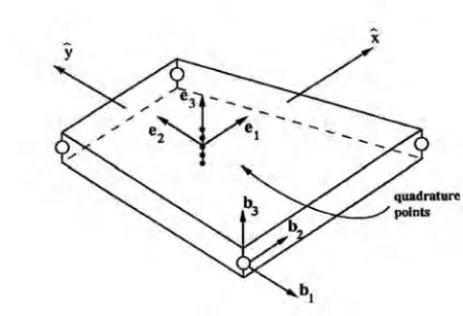
Figure 1. Three-dimensional Pipe Element Figure 2. Three-dimensional Plate/Shell Element
the contacting structures is the most efficient approach since a searching algorithm is not required. In contrast for problems in which the contact-impact locations are not know beforehand, a contact algorithm that can search and identify locations at which contact can occur is required.
The selection of a time integration scheme is critical to obtaining economical solutions. Because of the extremely short duration of the pipe impact event, explicit time integration is the most economical solution algorithm. The solution of the equations of motion does not require the inversion of a stiffness matrix, thus, resulting in an efficient scheme.
Finite Elements
This section gives terse descriptions of the elements used to simulate contact-impact of piping systems. The first element is a pipe element capable of undergoing large displacement in three-dimensional space. The second element is a quadrilateral plate element that can simulate the large deformation behavior of the wall of a pipe during impact. The material law associated with both of these elements is nonlinear elasto-plastic. Two contact elements were used in the simulations: node-to-line and node-to surface.
Pipe Element
For the global solution of a pipe whip event, the use of a pipe element capable of undergoing large displacements in three-dimensional space is required. The pipe element used in the NEPTUNE code is an enhanced version of a beam/pipe element developed by Belytschko and Schwer [7]. The element relations are developed in a co-rotational framework in which a rigid Cartesian coordinate system is embedded in each element so that it rotates with the element. With this approach, displacements and rigid body rotations of each element can be arbitrarily large, but the deformation of each element relative to the co-rotational coordinates must be small. This does not limit the formulation to small deformations but imposes the requirement that the number of elements used in the model be sufficiently large so that deformation of each element relative to its rigid Cartesian co-rotational system be small.
Plate Element
When the interest is to determine the local damage to a pipe, then it is necessary to use plate/shell elements to model the pipe wall. The number of elements required is significantly higher than using two-node pipe elements, but the local damage can be accurately accessed. The NEPTUNE code uses an enhanced version of the plate element proposed by Belytschko [8]. The formulation is based upon Midlin [9] theory of plates and uses a velocity strain formulation. The element is a bilinear four-node quadrilateral plate element based upon a one-point quadrature rule. Because of the use of the one-point quadrature, the element may exhibit hourglassing. To control the spurious modes, hourglass control [10] is employed.
Contact Elements
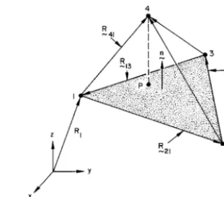
Figure 3. Node-to-Line Contact Element Figure 4. Node-to-Surface Contact Element
element in which two nodes are coincident with two nodes of a pipe element from one pipe and the third node is a node from a pipe element of another pipe. Thus, this element can only be used for problems with simple geometry and when the contact-impact location is known beforehand. The second contact element used below is a point-to-surface (tetrahedral) contact element. This element is employed when a pipe element would impact against a surface that is discretized with triangular elements. As shown in Fig. 4, the base of the tetrahedral is formed by the three nodes of a triangular element, which, for example, would used to model a concrete slab, and the apex is one node from a pipe element.
Solution Algorithm
Because of the transient nature of whipping pipes interacting with each other and/or surrounding structures, the most efficient time integration algorithm is the central difference scheme, which is an explicit integration algorithm. Typically, the time scale for contact-impact events is on the order of milli-seconds (ms). For energetic pipes, the impact results in nonlinear material response with sections of one or both pipes exceeding the yield stress. This algorithm does not require matrix inversion but the time step must be equal to or less than the Courant limit. Within the NEPTUNE code, contact can be modeled with contact elements and/or a contact algorithm.
An overview of the explicit time integration scheme is given in Table I. First the initial conditions are set. These could be the specification of the initial velocity fields for the pipes. The second step is to update the displacement vector from the initial velocity vector. With the updated configuration, strains can be computed and used in a constitutive relationship to compute stresses, which are used to compute the internal force vector. The external force vector can be composed of contributions from several sources. The first contribution comes from prescribed external loading. When the piping contains a moving fluid, external forces are generated from momentum changes when the fluid changes its flow direction. During contact-impact, external forces are generated in the contact zone. With the internal and external forces known, the equations of motion can be solved for the accelerations. The integration procedure is repeated as shown in Table I.
Table I. Flowchart for Explicit Integration of Equations of Motion with Contact-Impact
1 Set initial conditions 2 Update displacements
3 Compute internal force vector by looping over all elements Compute external force vector
• Add contribution to external force vector from external loads
• Add contribution to external force vector from momentum changes of the fluid inside piping
• Add contribution to external force vector from contact elements • Add contributions to external force vector from contact algorithm 4 Update accelerations
VALIDATION PROBLEMS AND RESULTS
Pipe-to-Pipe Impact
After the occurrence of a guillotine pipe break, it is conceivable that the whipping pipe would impact against an adjacent pipe. To validate the NEPTUNE code for this situation, numerical simulations were done and benchmarked against the experimental test results reported by Alzheimer et al. [4]. In particular, the simulations were performed for the Series I tests. The experimental setup is shown in Fig. 5 below, and it consists of two pipes: a swinging pipe and a target pipe. The swinging pipe was 116 inches long, and the pivot was located 80 inches from the contact point. The target pipe was resting on supports that were 108 inches apart. Both pipes were made from A106 Grade B steel, which is the most typical carbon steel in nuclear power plants. The following material properties were used in the analyses: density 7.34 x 10⁻⁴ lb-s2/in4, Young’s modulus 30 x 106 psi, Poisson’s ratio 0.3, yield stress 35 x 103 psi, plastic modulus 125.8 x 10³ psi, and tensile strength 60000 psi.
A finite element model was made that used 14 two-node
pipe elements to represent the swinging pipe, 12 pipe element to represent the target pipe and one node-to-line contact element. Since the point of contact between the two pipes is known before hand, the node-to-line contact element was used to capture the contact mechanics at impact. The “node” was the center node on the target pipe and the “line” was a pipe element of the swinging pipe. Thus, once contact was detected, penalty forces were applied to each pipe to prevent interpenetration.
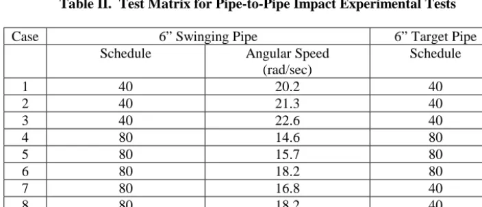
To start the simulation, the swinging pipe was positioned close to the target pipe but not in contact. Ref. [4] reported the experimental angular velocity for the swinging pipe just prior to impact, and that value was used to determine the velocity field of the swinging pipe. The velocity field was applied as the initial condition to the swinging pipe and the target pipe was initially at rest. Simulations were performed for the cases shown in Table II below. The test matrix consisted of combinations of 6 inch Schedules 40 and 80 steel pipes.
Table II. Test Matrix for Pipe-to-Pipe Impact Experimental Tests
Case 6” Swinging Pipe 6” Target Pipe
Schedule Angular Speed
(rad/sec)
Schedule
1 40 20.2 40
2 40 21.3 40
3 40 22.6 40
4 80 14.6 80
5 80 15.7 80
6 80 18.2 80
7 80 16.8 40
8 80 18.2 40
9 80 19.5 40
Figures 6 and 7 below show the deformed shape of the swinging and target pipes for Case 1. The swinging pipe is shown in Fig. 6, in which the point of impact and pivot point are defined. Figure 7 shows the heavily deformed shape of the target pipe, which is seen to have a maximum displacement of over 15 inches.
w
T arg et p ip e
S w in g in g p ip e
-20 -15 -10 -5 0 5 10
-40 -20 0 20 40 60 80
Global longitudial axis X, in
Displacements Z, in
point of pivot
impact zone
w
Figure 6. Deformed Shape of Swinging Pipe (Case 1). Figure 7. Deformed Shape of Target Pipe (Case 1).
0 15 30 45 60 75 90
0 0.1 0.2 0.3 0.4 0.5 0.6 0.7 0.8 0.9 1
Kinetic energy, xE+06 inlb
Bend angle, degrees
Swinging pipe, test Target pipe, test Swinging pipe, calculated Target pipe, calculated
0 15 30 45 60 75 90
0 0.1 0.2 0.3 0.4 0.5 0.6 0.7 0.8 0.9 1
Kinetic energy, xE+06 inlb
Bend angle, degrees
Swinging pipe, test Target pipe, test Swinging pipe, calculated Target pipe, calculated
(a) (b)
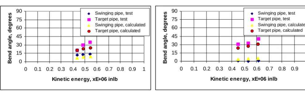
Figure 8. Comparison between experimental and calculated global bending angles: (a) Cases 1-3, 6 inch Schedule 40 impacting onto 6 inch schedule 40; (b) Cases 7-9, 6 inch Schedule 80 impacting against 6 inch Schedule 40.
Alzheimer et. al. [4] reported the values for global bend angles for each of the experimental test. Those values along with the bend angles obtained from the numerical simulations are shown in Fig. 8. Figure 8a shows the comparison for a 6 inch Schedule 40 swinging pipe impacting a 6 inch Schedule 40 target pipe. Table 1 indicates that three tests (Cases 1, 2 and 3) with these parameters were performed. The only difference between these three cases was the measured angular velocity of the swinging pipe just prior to contact. It is seen that for Case 3 the angular velocity (22.6 rad/sec) was 12% greater than for Case 1 (20.2 rad/sec) for the same conditions. This results in a 25% increase in swinging pipe kinetic energy for Case 3 over the kinetic energy of Case 1. Figure 8a shows that the computed bend angles are in good agreement with the measured angles from the tests. Both test and computed results show an increase in bend angle with an increase in initial kinetic energy.
The comparisons between experimental test results and simulation predictions for a 6 inch Schedule 40 pipe impacting onto a 6 inch Schedule 80 pipe are shown in Figure 8b. Here the spread in angular velocity was 25% which resulted in 55% variation in kinetic energy between Case 4 and Case 6. It is seen that the simulation results are in good agreement with the experimental test results. The results of global bending angle of both the target and swinging pipes showed good correspondence to experimental data, having in mind, that local crushing of pipes was not evaluated, since the beam-type pipe elements were used.
Pipe-to-Rigid Surface Impact
The next problem in the validation suite was a swinging pipe that was driven into a thick reinforced concrete plate [1, 3], which was considered a rigid surface. The 3 inch diameter Schedule 80 pipe was at 572o F at the start of the test and was made from A106 Grade B steel with the following properties: density 7.34 x 10⁻⁴ lb-s2/in4, Young’s modulus 29 x 106 psi, Poisson’s ratio 0.3, yield stress 32 x 103 psi, plastic modulus 85 x 103 psi, tensile strength 58 x 103 psi and ultimate strain of 31% . -20 -15 -10 -5 0
-60 -40 -20 0 20 40 60
Global longitudial axis Y, in
Displacements Z, in
left support right support
Figure 9. Geometry of Pipe Impact Experiment
The experimental setup is shown in Fig. 9, and comparisons were made with Test 5 reported in Ref. [3]. The length of the pipe, L1
, was 144 inches, the vertical extension length, L
2, was 8 inches, the radius was 4.5 inches and the distance, d1, fromthe bottom of the pipe to the surface of the non-deformable rigid structure was 8 inches.
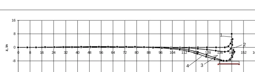
Two FE models were developed to simulate the response of the pipe impacting against a rigid surface. The first model employed the two-node pipe element and a point-to-line contact element. The second model used the four-node quadrilateral plate elements to discretize the entire pipe. The first model used 27 pipe elements (Fig. 10) to represent the pipe and 3 contact element between the pipe elbow and rigid surface. Loading, which was experimentally determined [3], was applied to the nodes in the elbow region. Figure 10 shows snapshots of the deformed shape of the pipe at several times during its dynamic response. It is clearly seen that the bending occurs in the region close to the elbow, and most of the remainder of the pipe is relatively straight. The numerical simulation indicated that the time to impact was 9.03 ms; the vertical velocity at impact was 1909 in/sec; the maximum impact force was 253,000 lbf ; and the duration of the impact was 0.93 ms.
The second model used a total of 4080 quadrilateral plate elements to model the entire pipe. Each circumferential cross-section was modeled with 24 elements. In order to capture the impact mechanics, node-to-surface contact elements (Fig. 4) were located between the pipe and rigid surface in the anticipated contact zone. The identical total loading used in the first model was distributed over a group of elements in the elbow region. Figure 11 shows the deformed shape of the pipe after impacting against the reinforced concrete slab. It is seen that the impact zone near the elbow of the pipe has undergone extensive plastic deformation and has been forced inward. The cross section geometry of the pipe in the impact zone is shown in Fig. 12, and it is seen that the original circular pipe, with a cross section area of 8.04 in2, has been deformed into a kidney shape, with a cross section area of 5.6 in2.
Figure 10. Snapshots of the Deformed Pipe at 0 ms, 5 ms, 9.03 ms (first impact), and the end of impact.
R4.5 L1
L2
d1
X
Z
-16 -8 0 8 16
0 8 16 24 32 40 48 56 64 72 80 88 96 104 112 120 128 136 144 152 160
x, in
z, in
1
2
Figure 11. Deformed Shape of Impact Zone
-10.00 -9.50 -9.00 -8.50 -8.00 -7.50 -7.00
-2.00 -1.50 -1.00 -0.50 0.00 0.50 1.00 1.50 2.00
X, in
Y, in
Figure 12. Kidney-Shaped Cross Section in the Pipe Impact Zone
A comparison between the results from numerical simulations using both the pipe element model and the plate/shell model with experimental test results is given in Table 3 below. It is seen that the time-to-impact measured during the test was 10 ms. The time to impact determined by the pipe element model simulation was 9.03 ms, and the time-to-impact for the shell model simulation was 8.17 ms. A value of 1,614 in/s was computed for the vertical impact velocity by an analysis reported in Reference [1]. Here vertical impact velocities of 1,909 in/s and 1,951 in/s were computed for the pipe model and shell model, respectively. The experimentally determined maximum impact force was 86,550 lbf compared to the pipe model
value of 253,000 lbf and the shell model value of 114,000 lbf . Since the shell model can capture the local elasto-plastic
Table 3. Comparison Between Results from Numerical Simulations and Experimental Test
Test Case Model Type Time to Impact, (ms)
Vertical Impact Velocity
(in/s)
Maximum Impact force
(lbf)
Impact Duration (ms)
Experiment 10.00 1,614 86,550 1.4
5 1 9.03 1,909 253,000 0.93
deformations of the pipe wall in the impact zone, it gives a better representation of the impact force. The last column of Table 3 compares the impact durations.
SUMMARY AND CONCLUSION
One of the concerns of the nuclear safety community is the consequence of a breach in a critical piping system and the effect on adjacent piping and surrounding structures. To a first order, these consequences can be evaluated by doing numerical simulations of whipping pipes following a guillotine pipe break. With the large advances in computing power, the interaction of whipping pipes with adjacent pipes and surrounding structures, such as equipment, concrete wall/floors, etc., can be evaluated economically through modeling and simulation. However, to have high confidence in the models and structural analysis software it is necessary to validate the computer codes used to perform the simulations.
Following an extensive literature search, a set of experiments was identified for use in validating Argonne’s NEPTUNE structural analysis computer code. The experiments included pipe impact, rigid surface impact and pipe-to-concrete slab impact. Numerical simulations of two of the experiments (pipe-to-pipe impact, pipe-to-rigid surface impact) were performed to validate the software. Models were developed to represent the respective piping systems and comparisons to experimental test results were made.
The conclusion drawn from the pipe-to-pipe comparison was that the two-node pipe element properly models the global behavior of a whipping pipe impacting a stationary pipe. The global pipe deformations, as measured by bend angle, closely replicate the experimental test results for nine cases that included various combinations of Schedules 40 and 80 six-inch pipes. For the pipe-to-rigid surface simulation, the plate/shell model was in good agreement with test results. These problems have validated the NEPTUNE code for use in pipe whip analyses and have shown the degree to which the numerical simulations can replicate experimental test results. Validation efforts are continuing through numerical simulations of the remainder of the problems from the validation suite.
ACKNOWLEDGEMENT
The work of the first author was performed under the auspices of the U.S. Department of Energy, Office of International Nuclear Safety and Cooperation, under Contract W-31-109-Eng-38. The work of the second author was performed at Argonne National Laboratory and supported by the IAEA/US Nuclear Safety Fellowship Program.
REFERENCES
1. Garcia J. L., Couard P., Sermet E., “Experimental Studies of Pipe Impact on Rigid Restrains and Concrete Slabs,”
SMiRT 7, Paper F2/1, 1983.
2. Carli F., Chouard P., Garcia J., “Pipe Impact on Concrete Slabs,” Proceedings of Conference Structural Engineering in Nuclear Facilities, Vol. 1, 1984, pp 123-141.
3. Hsu L. C., Kuo A. Y., Tang H. T., “Nonlinear Analysis of Pipe Whip,” SMiRT 8, Paper F1 4/6, 1985.
4. Alzheimer J. M., Bampton M. C. C., Friley J. R., Simonen F. A., “Pipe-to-Pipe Impact Program,” NUREG/CR-3231, PNL-5779, 1987.
5. Brunel L., Stromboni A., Lallement J., “Pipe to Pipe Impact Tests,” SMiRT 10, Vol. F, 1989, pp 65-74.
6. Kulak, R. F. and Fiala, C. "NEPTUNE: A System of Finite Element Programs for Three-Dimensional Nonlinear Analysis," Nuclear Engineering and Design, 106, 1988, pp. 47-68.
7. Belytschko T., Schwer L., “Large Displacement, Transient Analysis of Space Frames,” International Journal for Numerical Methods in Engineering, Vol. 11, 1977, pp 65-84.
8. Belytschko, T., Lin, J. I. and Tsay, C-S, “Explicit Algorithms for the Nonlinear Dynamics of Shells,” Computer
Methods in Applied Mechanics and Engrg., Vol. 42, 1984, pp. 225-251.
9. Mindlin, R. D., “Influence of Rotary Inertia and Shear on Flexual Motions of Isotropic, Elastic Plates,” J. of Applied Mechanics, Vol. 18, 1951, pp31-38.
10. Flanagan, D. and Belytschko, T., “A Uniform Strain Hexahedron and Quadrilateral with Orthogonal Hourglass Control,” Intl. J. for Numerical Methods in Engrg., Vol. 43, 1984, pp.251-276.
11. Kulak, R. F., "Adaptive Contact Elements for Three-Dimensional Fluid-Structure Interfaces," Eds., C. Y. Wang and T. B. Belytschko, Fluid-Structure Dynamics, ASME Publication PVP-Vol. 98-7, 1985, pp. 159-166.
12. Kulak, R. F., "Adaptive Contact Elements for Three-Dimensional Explicit Transient Analysis," Computer Methods