! " # # "$ % %#
& ''' (
Comparison of Supervised Classification Methods for Efficiently Locating Possible
Mineral Deposits using Multispectral Remote Sensing data
V. Joevivek*
Research scholar/ Centre for Geo-Technology Manonmaniam Sundaranar University
Tirunelveli, India [email protected]
N. Chandrasekar
Professor and Head/ Centre for Geo-Technology Manonmaniam Sundaranar University
Tirunelveli, India [email protected]
Abstract: Coastal landforms characterized by an accumulation of a wide range of sediment types and by many varied coastal environments. Sediment deposits around the central Tamilnadu coast contain significant amounts of heavy minerals and may attain concentrations of economic importance. The research work emphasize to locating possible heavy mineral deposits from multispectral imagery using supervised classification methods. We focused on soil prototype for locating possible minerals due to presence of placer deposits and absence of rock formations in our study area. The textural features were employed aiming at obtaining a highly separable class sets. Many supervised classification techniques are utilized in surface mineral investigation. Among them, several supervised techniques are analysed and the algorithm that best suit for the application is determined.
Keywords: Supervised classification, Multispectral image, Remote sensing, Textural features, Heavy minerals, Band ratios
I. INTRODUCTION
Remote sensing images are composed of a matrix of picture elements, which is represents natural and synthetic features of the whole or a part of the earth’s surface. Broadly, there are two types of remote sensing systems to record the information about any target. They are active sensing system and passive sensing system. These systems can be sub-classified by system parameters, namely, (1) platforms (airborne or spaceborne), (2) sensor configuration and filters, (3) spatial and spectral resolution. In this work, we used Landsat TM multispectral data for mineral potential mapping. The Landsat TM data can be collected by passive remote sensing system, and employ different bands in the visible, near infrared, middle infrared as well as thermal infrared regions. Classical analytical procedures for mineral potential mapping are available in the literature, for example [1-7]. Several of the more commonly used ones are briefly described here for locating possible heavy mineral deposits. Band ratio is a common technique that has been used for many years in remote sensing to display the mineral bearing areas [3, 4, 8]. The band ratio of B3/B1 result shows DN value of above 145 provides ferric iron oxide (limonite) areas. Similarly, Landsat TM 5/7 ratio shows Rich Al-OH areas [4,5]. Another image could be obtained assigning the ratio B3/B1 to Red, B5/B7 to Green and B5/B4 to Blue. In the resulted image, the yellow specifies the hydrothermally altered areas, the black identifies the water, the green with different chroma specifies the vegetation (dark green) and the clays-rich rocks (light green), the blue highlights sand and the red, pink or magenta area indicates some mineral rocks (iron oxides). The ratio B5/B7 to Red, B3/B1 to Green and (B5/B7)+(B3/ B1) to Blue shows bright areas are hydroxyl-bearing area, iron oxides and anomalous concentrations of both. Band ratio of B5/B4 to Red, B7/B4 to Green and B3/B7 to Blue shows brightest areas are hydrothermally altered area. Unfortunately, the above said methods may provide false alarm when the imagery having more noise or sometimes getting same reflectance of natural and synthetic objects. The advantage of band ratio method is to discriminate mineral bearing areas.
Another classical approach is principle component analysis. In general, the bands of PCA data are non-correlated and independent, and are often more interpretable than the source data [4, 6]. Because multispectral data bands are often highly correlated, PCA transformation is used to produce uncorrelated output bands. The first PCA band contains the largest percentage of data variance and the second PCA band contains the second largest data variance, and so on; the last PCA bands appear noisy because they contain very little variance, much of which is due to noise in the original spectral data. PCA is applied to the Landsat 5 image the resulting image has wide range of color that make the different lithological units easily discriminated [9]. This may be helpful for feature extraction process.
Beyond this, most of the researchers preparing their mineralogical maps from multispectral imagery based on pattern recognition and classification techniques [4, 10, 11, 12]. Many supervised and unsupervised classification methods are available in literature. We have employed mainly supervised classification techniques with awareness of its performance. These points will be discussed later at the proper places.
II. STUDY AREA AND DATA
Figure 1. The study area on Landsat 5 imagery
A. Geology of the study aera
The central Tamilnadu coast region has significant amounts of monazite, illmenite, rutile and garnet and a small amount of zircon and sillimanite. These minerals are found as placer deposits [1,2,3]. The nearest major sediment source for this coastal segment is the Cauvery river drains. The Cauvery river drains primarily the Precambrian gneisses and charnockites in the upstream and the cretaceous of Trichirappalli in the downstream.
B. Description of the Landsat TM5 data
The Landsat 5 satellite had the Thematic Mapper (TM) sensor as well as the MSS, are inclined 98 degrees, have a repeat cycle of 16 days and have an equatorial crossing of 9:45am local time. The nominal altitude of LANDSAT 5 is 705km. Spectral coverage of Landsat 5 records data in a wide bandwidth range (Band 1: 0.45-0.52µm, Band 2: 0.52-0.60µm, Band 3: 0.63-0.69µm, Band 4: 0.76-0.90µm, Band 1: 1.55-1.75µm, Band 6: 10.4-12.5µm, Band 7: 2.08-2.35µm). First three bands are in visible region, band 4 in near infrared region, band 5 and 7 in mid infrared region and band 6 in thermal infrared region. Band 6 particularly designed for vegetation analysis and it has very less spatial resolution (120m/pixels). Due to these reasons, we considered six bands except band 6 for locating mineral bearing areas.
C. Preprocessing
Preprocessing is an important and diverse set of image preparation programs that act to offset problems with the band data and recalculate DN values that minimize these problems [20]. Offset (banding defect) restoration could be solved by histogram equalization technique. Theory behind is calculate the average histograms of the brighter and darker bands. The histograms are then adjusted to a uniform average brightness level for both sets of scan lines [4]. Secondly, FLAASH (Atmospheric Correction Of Hyperspectral /Multispectral Imagery) algorithm for the Landsat 5 data much helpful to remove atmospheric noise factors. Subsequent analyses were then based on these preprocessed Landsat 5 images.
III. ALGORITHM
This section describes a framework to design an algorithm for locating possible mineral potential area using
Landsat 5 data. In this work, Area of Interest from 11º15’N-11º35’N and from 79º30’E-79º50’E. A geological map of the said region was provided by Geological Survey of India [21]. The given geological map includes all soil types present in the study area. In other hand, PCA and band ratios of our imageries were determined.
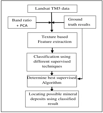
Being guided by combination of geological map, Band ratios and PCA results some windows with homogeneous ground cover were selected (region of interest) and features of Landsat 5 bands corresponding to these areas are used training samples. The search of efficient supervised classification technique is achieved by cross validation accuracy. The validation based on how much classifier can separate class sets as well as how much it gives prediction accuracy. In addition, time elapsed parameter also considered. Finally, possible mineral deposit locations were drawn from best classifier results. Fig. 2 shows systematic structure of above said procedure.
Figure 2. Framework
IV. DATA REFINING
Underlying requirement of supervised classification techniques is that analyst must have either sufficient knowledge about the prototypes representing different classes of interest, or sufficient known pixels of each class that representative prototype can be developed for these classes [4, 10] . In this work prototype means different soil types. This set of pixels from which prototype signature is generated is known as training data; and the steps of determining class signature is often called training. The training samples were collected based on four distinguished aspects namely, (i) Visual interpretation with ground truth results, (ii) Geological map, (iii) Band ratios, (iv) PCA results.
Landsat TM5 data
Band ratio
Texture based Feature extraction
Classification using different supervised
techniques
Determine best supervised Algorithm
Ground truth results
Locating possible mineral deposits using classified
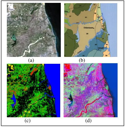
[image:2.612.330.540.246.476.2]Figure 3. Original image (false colour composite), (b) geological soil map, (c) band ratio image, (d) PCA image
Yellow colour in figure 3(c) stands for Iron-oxide bearingareas. Similarly, red colour in figure 3(c) indicates composite of clay, iron oxide and vegetated areas. In figure 3, Black body areas in 3(c) as well as light violet areas in 3(d) shows imperfectly drained, cracking clay soils. Blue colour in both 3(c) and 3(d) correspond to water bodies. With the above reference, feature values are extracted from source imagery (i.e., original inage).
In our experiment, we consider eight different classes namely, non-saline (soil 1), saline and sodic in patches (soil 2), coastal alluvial soil (soil 3), floodland soil (soil 4), red gravelly loam soil (soil 5), lateritic gravelly soil (soil 6), vegetation areas and water bodies. Different soil contains different types of minerals. The possible minerals of soil types which we observed from geological survey and literatures [14-19] are described below.
• Soil 1: possibilities of mirabilite, glauberite, gypsum, calcite, dolomite, ulexite, analcime • Soil 2: dominance of illite, fairly high amount of
semectite, some chlorite, mixed layer mineral and small amount of kaolinite.
• Soil 3: composed of a mixture of hydrated oxides of aluminum and iron with small amounts of the oxides of manganese, titanium.
• Soil 4: variable amounts of calcium carbonate and soluble salts
• Soil 5: soluble salts of calcium, magnesium and sodium to the surface of soil
• Soil 6: available phosphorus but rich in calcium carbonate
For these classes training samples have been picked up from source image in the form of textural features. We suggest a set of eight textural features which can be extracted from each of the gray-tone spatial-dependence matrices (GLCM) [22]. The following equations define these features.
• Mean: • Variance: • Homogeneity: • Contrast: • Dissimilarity: • Entropy: • Second moment: • Correlation: Notation
p(i,j) - (i,j)th entry in a normalized gray-tone spatial dependence matrix, = P(i,j)/R
Ng - Number of distinct gray levels in the quantized image
µx, µy, x, y - Mean and Standard deviations of px and py.
Where,
px(i) - ith entry in the marginal-probability matrix obtained
by summing the rows of p(i,j), =
py(i) =
We assigned our multispectral data consisted of small image blocks of size 3X3 and gray tones of the images were equal-probability quantized into 64 level. The textural features for the image blocks were calculated from distance 1 gray level co-occurrence matrix.
Broadly, we could not evaluate all the supervised classifier algorithms. In other hand, some of the commonly used algorithms were evaluated namely, Parallelepiped, Mahalanobis distance, Maximum likelihood, Minimum distance, Support vector machine, Neural networks. Theory of above said supervised algorithms are described in [4, 10, 13]. Training and testing performance of different supervised classification techniques are briefly described in subsequent sections. It should be noted that whatever be the classification strategy, training data should reflect their separability in the feature space for useful results.
V. CLASSIFICATION RESULTS OF VARIOUS SUPERVISED
CLASSIFICATION TECHNIQUES
A. Training performance
In this section, we present the results of our studies on the training performance of the various supervised techniques. We have 560 different feature vectors and we took 60% for learning and 40% for testing. We assigned
(a) (b)
(c) (d)
= =
=
g g N i N j gj
i
P
N
t
1 11
(
,
)
1
−
=
i jj
i
p
i
t
2(
µ
)
2(
,
)
−
+
=
i jj
i
p
j
i
t
(
,
)
)
(
1
1
2 3 = − = = = = n j i j i P n t g g g N i N j N n 1 1 0 2 4 ) , ( = =−
=
g g N i N jj
i
j
i
p
t
1 15
(
,
)
−
=
i jj
i
p
j
i
p
t
6(
,
)
log(
(
,
))
{
}
=
i jj
i
p
t
7(
,
)
2phase I as a combination of mean, variance. Similarly, Phase II as addition of homogeneity, contrast with phase I. Phase III have 6 textural features that is Phase I+ Phase II+ dissimilarity and entropy, Phase IV contains 8 textural features. Phase V is different from others because it has 8 textural features with spectral values of all the 6 bands. Cross validation has been done for different supervised algorithms with various phase levels. The result has been plotted in Fig.4.
From the plot, we understood that Parallelepiped gives poor result, Minimum distance and Mahalanobis distance shows similar results, SVM and maximum likelihood are comparatively same. The result obtained from neural network is significant one. It started well but getting less accuracy when the feature level increase.
[image:4.612.319.558.61.231.2]We attempted a textural classification on the multispectral data and achieved a classification accuracy of 68-79 percent on the test set. This result, compared with the 85-95 percent classification accuracy achieved using a combination of spectral and textural features, shows that a significant improvement in the classification accuracy might result if the spectral features are used as additional inputs to the classifier.
Figure 4. Cross validation accuracy for various supervised algorithms
B. Classification results
The training data set is classified using different classification algorithms. In this paper SVM algorithm programmed in MATLAB and remaining techniques performed in ENVI with same datasets [23, 24]. The classification results are shown in Table 1.
From the results in table 1, it is understood that SVM based classification and Mahalanobis Distance are the two supervised algorithms that gives good classification accuracy. Since the data considered here is a higher dimensional one, the classification accuracy of neural networks is very less. In this work SVM based classification is taken for further analyses. The subsequent section deals with SVM based classification technique.
Table I. Classifcation results of various supervised techniques
Supervised methods
Classification results
Classified Accuracy (in percentage)
Kappa coefficient
Time elapsed (Sec)
Parallelepiped
Minimum distance
Mehalonobis distance
Maximum likelihood
Neural (MLP)
SVM
73.4537
83.6097
85.8898
92.9752
79.1629
93.4240
0.7279
0.8281
0.8511
0.9213\
0.7845
0.9258
13.52
12.23
12.39
14.63
>120
14.56
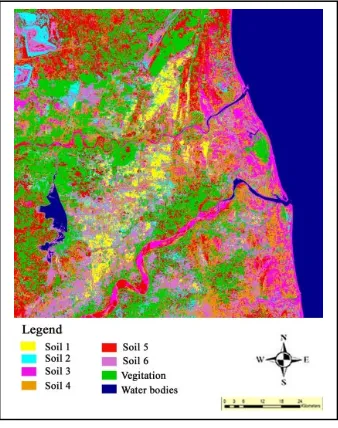
C. SVM based classification
[image:4.612.59.267.288.495.2]In support vector machines, the learning machine is given a set of examples (training data) and its associated class labels. SVM tries to construct a maximally separating hyperplane between classes, thus by differentiating the classes. The parameter ‘C’ controls the weightage for maximum margin requirement and sum of error. Maximum margin and minimum error are two contradictory things and the value ‘C’ controls these parameters to achieve optimum results [25]. The best value of ‘C’ is found out by cross validation. However the optimization problem is converted into its dual and solved. The classified image using linear kernel is shown in Fig. 5.
Figure 5. SVM based Classification result
[image:4.612.353.522.399.613.2]of correctly classified classifier pixels per class/total classifier pixels per class). The overall accuracy is calculated by summing the number of pixels classified correctly and dividing by the total number of pixels. The result showed
that the overall accuracy of SVM classifier is 93.45% as well as kappa co-efficient is 0.9245.
Table II. Classification accuracy
Classified results
Ground truth (Percent)
Soil1 Soil2 Soil3 Soil4 Soil5 Soil6 Veg. Wat Tot Comm Omi Prod User
Soil1 Soil2 Soil3 Soil4 Soil5 Soil6 Veg. Water Tot 84.58 5.53 3.57 0.36 0.00 5.97 0.00 0.00 100.00 42.19 37.49 4.49 4.02 0.13 11.27 0.40 0.00 100.00 31.12 3.03 48.09 14.16 0.00 3.60 0.00 0.00 100.00 0.00 3.27 10.28 83.18 1.40 1.87 0.00 0.00 100.00 0.00 0.00 0.48 2.70 96.50 0.16 0.16 0.00 100.00 23.62 7.69 2.93 4.97 0.07 60.38 0.34 0.00 100.00 0.00 0.00 0.00 0.08 0.04 0.20 99.67 0.00 100.00 0.00 0.00 0.08 0.00 0.00 0.14 0.03 99.74 100.00 6.34 2.22 1.80 1.33 1.77 3.46 7.06 76.03 100.00 56.90 27.31 31.41 61.39 1.14 26.21 0.78 0.00 15.42 62.51 51.91 16.82 3.50 39.62 0.33 0.26 84.58 37.49 48.09 83.18 96.50 60.38 99.67 99.74 43.1 72.6 68.6 38.6 98.9 73.8 99.2 100
VI. CONCLUSION
This paper emphasized possibility of the geological resources especially the mineral resources in the central Tamilnadu coast using Landsat 5 multispectral remote sensing data. From all the supervised learning algorithm, SVM is considered give higher accuracy for our dataset. The accuracy of Maximum likelihood is comparable. Even though linear kernel is considered less powerful than polynomial and RBF kernels, linear kernel gives good prediction accuracy. This is because of the higher dimensionality of our data set and sometimes the use of powerful kernels causes overfitting of training data. Interpretation of resultant image with soil map shows clearly discriminated soil types. Even though textural features are time costly, it provides maximum separable class sets. From results, we found that our study area has possibilities of heavy minerals such that alluvial and sediment minerals. The research provided truthful results of possible mineral deposits even multispectral imagery having low spectral resolution. In order to improve the accuracy we suggest a method, which is corner estimation in classified imagery using fuzzy membership function.
VII. ACKNOWLEDGMENT
We thank prof. N. Mukunda, Chairman, Science education panel, IASc, Bangalore and Prof. Malay. K. Kundu, Dr. Uma Shankar, Machine Intelligence Unit, ISI, Kolkata for their fullest guidance and encouragement for the present work.
VIII. REFERENCES
[1] M.J. Abrams, D. Brown, L. Lepley and R. Sadowski, ”Remote sensing for porphyry copper deposits in southern Arizona”, Economic Geology, Vol. 78, 1983, pp. 591– 604.
[2] M.J. Abrams, D.A. Rothery and A. Pontual, “Mapping in the Oman Ophiolite using enhanced Landsat Thematic Mapper images”, Tectonophysics, Vol. 151, 1988, pp. 387–401.
[3] M. Sultan, R. Arvidson, and N.C. Sturchio, “Digital mapping of ophiolite melange zones from Landsat Thematic Mapper TM data in arid areas: Meatiq dome, Egypt”, Geological Society of America Annual Meeting, Abstracts with Programs, 1986, 18: 766.
[4] F. Sabins, RemoteSensing: Principlesand Interpretation, third ed., 1997, 494 p.
[5]
[6]
[7] M.G. Abdelsalam and R.J. Stern, “Mineral exploration with satellite remote sensing imagery: examples from Neoproterozoic Arabian shield”, Journal of African Earth Sciences, 1999, 28, 4a.
[8] L.C. Rowan and J.C. Mars, “ Lithologic mapping in the Mountain Pass, California area using Advanced Spaceborne Thermal Emission and Reflection Radiometer (ASTER) data”, Journal of Remote Sensing of Environment, Vol. 84(3), 2003, pp.350-366.
[9] S. Gad and T.M. Kusky, “Lithological mapping in the Eastern Desert of Egypt, the Barramiya area, using Landsat thematic mapper (TM)”, Journal of African Earth Sciences, Vol. 44, 2006, pp.196–202.
[10] Alexandru Imbroane, Cornelia Melenti and Dorian Gorgan, “Mineral Explorations by Landsat Image Ratios”, Ninth International Symposium on Symbolic and Numeric Algorithms for Scientific Computing, 2009, pp.335-340.
[11] Reda Amer, Timothy Kusky, Paul C. Reinert and Abduwasit Ghulam, Image Processing and Analysis Using Landsat Etm+ Imagery for Lithological Mapping at Fawakhir, Central Eastern Desert of Egypt, ASPRS 2009 Annual Conference, Baltimore, Maryland, March 9-13, 2009.
[12] A. John Richards, Xiuping Jia“Remote Sensing Digital Image Analysis - An Introduction” 4th ed., 2006.
[13] Sylvia S. Shen and Paul E. Lewis (editors and chairs), “Algorithms and Techniques for Multispectral Hyperspectral and Ultraspectral Imagery X”, Proceedings of SPIE, 12-15 April 2004.
[14] F. Mark Denson and Stephen E. Plummer, “Advances in Environmental Remote sensing”,1995.
[15] S. Mark Nixon and S. Alberto Aguado, “Feature Extraction & Image Processing”, Second edition, reprinted June 2008
[16] N.J. Angusamy, J. Dajkumar Sahayam, M. Suresh Gandhi, and G.V. Rajamanickam, “Coastal placer deposits of central Tamil Nadu”, India. Mar. Geo-Resour. Geotech. Vol. 23,2005, pp.137-174.
[17] N. Chandrasekar, “Beach placer mineral exploration along the Central Tamilnadu Coast”, Unpublished Ph.D.thesis, Madurai Kamaraj University, Madurai, 1992.
[18] Chandrasekar, and G.V. Rajamanickam, “Nature of distribution of heavy minerals along the beaches of central Tamilnadu coast”, Jour. Indian Association of Sedimentologists, Vol. 20, No. 2, 2001, pp. 167-180.
[19] J. Floor Anthoni, Soil geology, 2000, http://www.seafriends.org.nz/enviro/soil/geosoil.html
[21] Environment of earth, http://environmentofearth.wordpress.com/category/soil/
[22] Morro Bay, Image processing and interpretation- tutorial, http://rst.gsfc.nasa.gov/Sect1/
[23] Soil map provided by geological society of India, http://eusoils.jrc.ec.europa.eu/esdb_archive/eudasm/asia/li sts/cin.htm
[24] M .Robert haralick, K. Shanmugam and Its’hak dinstein, Texture features for image classification, IEEE Transactions on sytems, man, and cybernetics, vol. Smc-3, no.6, november 1973.
[25] ENVI version 4.5, ITT Visual Information Solutions. http://www.ittvis.com.
[26] MATLAB version 7.3.0.267(R2006b) August 03, 2006. Copyright 1984-2006, The MathWorks,Inc. Protected by U.S. patents. http://www.mathworks.com