N-term Karatsuba Algorithm and its
Application to Multiplier designs for
Special Trinomials
YIN LI1, YU ZHANG1, XIAOLI GUO1AND CHUANDA QI1.
1
Department of Computer Science and Technology, Xinyang Normal University, Xinyang, 464000 P.R. China
Corresponding author: Yin Li (e-mail: [email protected]).
This work was supported by the National Natural Science Foundation of China (Grant No. 61402393, 61601396) and Shanghai Key Laboratory of Integrated Administration Technologies for Information Security (No. AGK201607).
ABSTRACT In this paper, we propose a new type of non-recursive Mastrovito multiplier forGF(2m)
using an-term Karatsuba algorithm (KA), whereGF(2m)is defined by an irreducible trinomial,xm+xk+ 1, m=nk. We show that such a type of trinomial combined with then-term KA can fully exploit the spatial correlation of entries in related Mastrovito product matrices and lead to a low complexity architecture. The optimal parameternis further studied. As the main contribution of this study, the lower bound of the space complexity of our proposal is aboutO(m22 +m3/2). Meanwhile, the time complexity matches the best
Karatsuba multiplier known to date. To the best of our knowledge, it is the first time that Karatsuba-based multiplier has reached such a space complexity bound while maintaining relatively low time delay.
INDEX TERMS N-term Karatsuba Algorithm, Specific trinomials, Bit-parallel Multiplier
I. INTRODUCTION
The finite fieldGF(2m)arithmetic has many applications in
cryptography and error-correcting code [1], [2]. For instance, one of the most important applications of GF(2m) is the
elliptic cure cryptosystem (ECC) [3]. Among the GF(2m)
arithmetic operations, multiplication is of most importance because other costly operations such as exponentiation and inversion can be carried out by iterative multiplications. Therefore, it is necessary to design highly efficient multipli-ers forGF(2m)multiplication.
The choices of the field basis and irreducible polynomials are crucial to multiplier design. Compared with other bases, polynomial basis (PB) is more promising in the sense of flexibility in irreducible polynomial selection and hardware optimization [9]. Moreover, some variations of polynomial basis, e.g., shifted polynomial basis (SPB) [5], [13] and generalized polynomial basis (GPB) [10], are proposed as well to optimize the multiplier architecture further. Among these irreducible polynomials in use, irreducible trinomial is one of the most common considerations. During recent years, many bit-parallel multiplier using PB have been proposed for GF(2m) generated with an irreducible trinomial [7], [12],
[16], [17], [27].
Generally speaking, the PB multiplication consists of two steps: polynomial multiplication and modulo reduction. The polynomial multiplication can be optimized using a divide-and-conquer algorithm such as Karatsuba algorithm (KA) [4], [18]. Such an algorithm saves coefficient multiplications
at the cost of extra additions compared to the school-book method. Thus, it can be easily adopted to design efficient GF(2m) multipliers. Specifically, there exists a class of
Karatsuba based multipliers, named as non-recursive Karat-suba multiplier, only apply KA once in the polynomial multiplication and obtain a trade-off between the space and time complexities. During recent years, several non-recursive Karatsuba multipliers have been proposed for various type of irreducible polynomials [14], [15], [21], [24], [28]. On one hand, such multipliers cost several more XOR gates delay compared with the fastest bit-parallel multiplier known to date [6], where no divide-and-conquer algorithm is applied. On the other hand, the space complexities of these multipliers are roughly reduced by 1/4.
Empirically, non-recursive Karatsuba multipliers focusing on specific irreducible polynomials usually have better space and time complexity than the ones for general polynomial-s. Such polynomials include equally-spaced trinomial (ES-T) [28], all-one polynomial (AOP) [15], etc. Recently, we explore another special form of trinomial xm +xm
3 + 1
name this type of trinomial asn-spaced trinomial. Obviously, this type of trinomial is EST ifn= 2. Shou et al. [26] have already investigated the development of the bit-parallel mul-tiplier for this trinomial using an-term Karatsuba algorithm. But their scheme requires 3 more XOR gate delays compared with the fastest one. In this paper, we apply an-term Karatsu-ba algorithm along with the shifted polynomial Karatsu-basis (SPB) to simplify the field multiplication. Mastrovito approach is utilized for polynomial reduction. It is demonstrated that the corresponding Mastrovito matrices for different parts of the field multiplication have relatively simpler forms, which lead to an efficient architecture. Moreover, we also give the explic-it formulae wexplic-ith respect to the space and time complexexplic-ity of the corresponding multipliers. As a result, the lower bound of our proposal costs approximatelyO(m22+m3/2)circuit gates
compared with the fastest bit-parallel multipliers, while its time delay matches the Karatsuba based multipliers known to date.
The rest of this paper is organized as follows: In Section 2, we briefly review the n-term Karatsuba algorithm, the SPB representation and some pertinent notations. Then, we present a new bit-parallel multiplier architecture forn-spaced trinomial in Section 3. After that, a small example is given. Section 4 presents a comparison between the proposed mul-tiplier and some others. More discussion about the optimal parameter is also given. Finally, some conclusions are drawn.
II. PRELIMINARY
In this section, we briefly review some important notations and related algorithms that used throughout this paper.
A. IRREDUCIBLEN-SPACED TRINOMIAL
We first consider the existence of the irreducible trinomial xm+xk+ 1, m=nkwhich are used to define the finite field GF(2m). The following lemma is useful.
Lemma 1. [2] Let f1(x), f2(x),· · ·, fN(x) be all the
distinct monic irreducible polynomial over Fp of degree m
and ordere. Let t ≥ 2be an integer whose prime factors divideebut not pme−1. Assume also thatpm ≡ 1 mod 4if
t ≡ 0 mod 4. Thenf1(xt), f2(xt),· · · , fN(xt)are all the
distinct monic irreducible polynomials inFp[x]of degreem·t
and ordert·e.
Lemma 1 provides a way to construct an irreducible trino-mial of higher degree, i.e., xnk+xk + 1, from the known
irreducible trinomialxn+x+ 1. If a trinomialxn+x+ 1is
irreducible over F2, one can find an integerk that satisfies
the above condition, to construct an irreducible trinomial xnk +xk + 1. For example, it is easy to check that both
x3+x+ 1andx4+x+ 1are irreducible. Meanwhile, their
orders are 7 and 15, respectively. It follows thatx3k+xk+ 1
(k = 7i) andx4k+xk+ 1(k = 3i×5j, i, j ≥0)are all
irreducible.
B. SHIFTED POLYNOMIAL BASIS
The shifted polynomial basis (SPB) [13] actually is a varia-tion of the polynomial basis. This novaria-tion is originally applied in the field GF(2m)generated with irreducible trinomials, and then pentanomials [5]. In this study, we consider the field GF(2m) generated by a n-spaced trinomial f(x) =
xnk + xk + 1. Let x be a root of f(x), and the set
M ={xnk−1,· · · , x,1}constitutes a polynomial basis (PB).
Then, the SPB can be obtained by multiplying the setM by a certain exponentiation ofx:
Definition 1. [13] Letvbe an integer and the ordered set
M ={xnk−1,· · ·, x,1}be a polynomial basis ofGF(2m)
overF2. The ordered setx−vM :={xi−v|0≤i≤nk−1} is called the shifted polynomial basis with respect toM.
Under SPB representation, the field multiplication can be performed as:
C(x)x−v=A(x)x−v·B(x)x−vmodf(x).
If the parameterv is properly selected, the field multiplica-tion using SPB representamultiplica-tion is simpler than that using PB representation, especially for the field define by irreducible trinomial or some type of pentanomials [5]. This character-istic directly lead to a more efficient Mastrovito multiplier which has lower time complexity compared with classic one using PB. Furthermore, it has been proved that the optimal value ofviskork−1for trinomials [13]. To construct an efficient multiplier forn-spaced trinomials, we choosev=k and use this denotation thereafter.
C. N-TERM KARATSUBA ALGORITHM
The classic Karatsuba algorithm multiplies two 2-term poly-nomials using three scalar multiplications at the cost of one extra addition. Then, Weimerskirch and Paar [8] proposed a slightly generalized algorithm for the polynomial multiplica-tion with arbitrary degree. This algorithm has the same idea as the classic one. We denote such an algorithm asn-term KA (n > 2). Provide that there are two polynomials of degree n−1overF2:
A(x) = n−1 X
i=0
aixi, B(x) = n−1 X
i=0
bixi.
The n-term KA for polynomial multiplication AB is as follows:
• Compute for eachi= 0,· · · , n−1,
Ei=aibi.
• Compute for eachi= 1,· · · ,2n−3and for alls, twith s+t=iandn > t > s≥0,
Es,t= (as+at)(bs+bt).
• The coefficients ofD(x) =A(x)B(x) =P2i=0n−2dixi
can be computed as
d0=E0,
d2n−2=En−1,
di=
P
s+t=i, n>t>s≥0
Es,t+P s+t=i, n>t>s≥0
(Es+Et)(oddi),
P
s+t=i, n>t>s≥0
Es,t+P s+t=i, n>t>s≥0
(Es+Et)+Ei/2(eveni),
wherei= 1,2,· · ·,2n−3.
The correctness proof about above formulae can be found in [8]. Merge the similar items for Ei,(i = 0,1,· · ·, n−1),
D(x)is rewritten as:
D(x) =En−1(x2n−2+· · ·+xn−1) +En−2(x2n−3+
+· · ·+xn−2) +· · ·+E0(xn−1+· · ·+ 1)
+P2n−3
i=1 (
P
s+t=i, n>t>s≥0
Es,t)xi.
(1)
One can easily check that the above formula costs about O(n22) coefficient multiplications and O(5n22) additions. Compared with classic KA, the n-term KA saves more coefficient multiplications at the expense of more coeffi-cient additions. Besides Weimerskirch and Paar’s algorithm, Montgomery [20] and Fan [19] proposed more alternative Karatsuba-like formulae. Their formulae aim to decrease as many coefficient multiplications as possible. These formu-lations usually contain complicated linear combinations of the coefficients, which will lead more gates delay for the bit-parallel architecture. Thus, we prefer to utilize the above algorithm to develop bit-parallel multiplier.
In Section 3, we investigate the construction of non-recursive Karatsuba algorithm using n-term KA for the n -spaced trinomial. Our main strategy is analogous to that in [24], which combines Mastrovito approach andn-term KA. Therefore, some notations pertaining to matrices and vectors are used as well. Note that these notations have already been presented in [9], [24].Z(i,:),Z(:, j)andZ(i, j)represent the ith row vector,jth column vector, and the entry with position
(i, j)in matrixZ, respectively.Z[ i]represents cyclic shift of Zby upperi rows. Z[ i] represents appendingi zero vectors to the top ofZ.
III. EFFICIENT MULTIPLIER BASED ONN-TERM KARATSUBA ALGORITHM
In this section, we present an efficient non-recursive Karat-suba multiplier forn-spaced trinomial xnk+xk+ 1 using
SPB representation. We firstly investigate the structure of the product matrix for polynomial multiplication based on n-term KA. Then, reduced matrices are calculated using Mastrovito approach. Accordingly, we propose the relat-ed multiplier architecture. It is shown that corresponding matrix-vector multiplications can be implemented efficiently forn-spaced trinomial. The space and time complexity of the corresponding multiplier is also discussed.
Provide that the finite field GF(2m) is generated with an irreducible trinomial xm+xk + 1, m = nk, the field
elements are represented using SPB. Applying n-term KA as presented previously, we partition two arbitrary field ele-mentsA=Pm−1
i=0 aixi−k, B =P m−1
i=0 bixi−k intonparts
with each part consisting ofkbits. More explicitly,
A=An−1x(n−2)k+An−3x(n−3)k+· · ·+A1+A0x−k,
B=Bn−1x(n−2)k+Bn−3x(n−3)k+· · ·+B1+B0x−k,
whereAi = P k−1
j=0aj+(i−1)kxj, Bi = P k−1
j=0bj+(i−1)kxj,
fori= 0,1,· · ·, n−1.
Then, we multiply AandB using then-term Karatsuba algorithm presented in Section 2 and do following transfor-mation:
AB=En−1·x(n−2)k+En−2·x(n−3)k+· · ·+E1+
E0·x−k
·h(x) +
2n−3
X
i=1
X
s+t=i, n>t>s≥0
Es,t
xik−2k, (2)
whereh(x) =x(n−2)k+x(n−1)k+· · ·+1+x−k,Ei=AiBi
(i= 0,1,· · · , n−1) andEs,t = (As+At)(Bs+Bt). We
partition the above expression into two parts, i.e.,
S1=(An−1Bn−1x(n−2)k+· · ·+A1B1+A0B0x−k)h(x),
S2= 2n−3
X
i=1
X
s+t=i, n>s>t≥0
Es,t
xik−2k,
and compute them independently. Thus, the field multiplica-tionC=ABmodf(x)now is rewritten as
C= (S1+S2) modf(x).
In order to apply Mastrovito approach, we have to rewrite both S1 and S2 into matrix-vector forms and then reduce
those matrices. Please note that m = nk and thus corre-sponding product matrices are more complicated than those presented in [24], [25]. The following subsections give the details.
A. COMPUTATION OFS1MODULOF(X) Since
S1=(An−1Bn−1x(n−2)k+· · ·+A1B1+A0B0x−k)h(x) =An−1h(x)Bn−1x(n−2)k+· · ·+A0h(x)B0x−k,
it is clear that S1 in fact consists of n parts, each of
which can be recognized as a shift of Aih(x)Bi, for i = 0,1,· · ·, n−1. Through constructing the matrix-vector form ofAih(x)Bi, i= 0,1,· · · , n−1, we can develop the
matrix-vector form ofS1. It is noted that
Aih(x)Bi= (Aix(n−2)k+· · ·+Ai+Aix−k)·Bi.
and bi represents the coefficient vector of Bi(x). Then,
Aih(x)Bi=Ai·bi, where
Ai=
−k
.. . .. .
nk−1
Ai,L Ai,L+Ai,H
.. .
Ai,L+Ai,H
n−1
Ai,H
.
The labels on the left side indicate the exponent of indetermi-natexfor each row inAi, which range from−ktonk−1.
However, we check that the degrees of xinAih(x)Bi are
actually in the range[−k, nk−2]. But the last row ofAiis
0, which does not affect the result. The matricesAi,H and Ai,Lare bothk×ktriangular Toeplitz matrix, i.e.,
Ai,L=
aik+0 0 · · · 0
aik+1 aik+0 · · · 0
..
. ... . .. ...
aik+k−1 aik+k−2 · · · aik+0
,
and
Ai,H=
0 aik+k−1 · · · aik+1 0 0 · · · aik+2
..
. ... . .. ...
0 0 · · · aik+k−1
0 0 · · · 0
,
fori= 0,1,· · ·, n−1.
Accordingly, thesensubmatrix-vector multiplications can constitute a bigger matrix-vector multiplication pertaining to S1, denoted byAS1·b. More explicitly,
S1=AS1·b=AS1·[b0,b1,· · · ,bn−1] T
=
A0 0k×k · · · 0k×k
0k×k A1 . .. 0(m−2k)×k
0(m−2k)×k 0(m−2k)×k · · · An−1
×
b0, .. .
bn−1
.
(3) For simplicity, we do not write the degree labels of the product matrix here. Notice thatdeg(AiBih) =nk−2, i= 0,1,· · · , n−1, we havedeg(S1) =nk−2 + (n−2)k= 2m−2k−2. One can check that the degrees of the terms of S1are in the range[−2k,2m−2k−2]. Based on Mastrovito
scheme,S1needs a further reduction byf(x). The following
reduction rule is applied:
xi=xm+i+xi+k, fori=−2k,· · ·,−k−1;
xi=xi−m+xi−m+k, fori=m−k, m−k+1,
· · · ,2m−2k−2. (4)
The reduction can be regarded as the construction of the Mas-trovito matrix fromAS1 according to (4). Let MS1 denote
the Mastrovito matrix related toS1. In order to analyze the
organization ofMS1, we introduce a lemma, which is the key
step toward the development of the multiplier architecture.
Lemma 2. Provide thatAis an arbitrary (2m−1)×m
matrix andbis am×1vector overF2. The Mastrovito matrix M related toA·bmoduloxm+xk + 1using (4) can be
obtained as follows:
M=M1+M2,
where
M1= [A(1,:)T+A(m+1,:)T,A(2,:)T+A(m+2,:)T, · · ·,A(2m−1,:)T+A(m−1,:)T,A(m,:)T][ k], (5)
and
M2= [A(1,:)T,· · ·,A(k,:)T,A(k+m+1,:)T, · · ·,A(2m−1,:)T,0]. (6)
Proof. We notice that the product matrix A here includes
2m − 1 rows with each row corresponding the degree from −2k to 2m−2k−2. Clearly, the first k rows and the last m − k − 1 rows correspond to the term de-grees that are out of the range [−k, m − k −1]. Based on (4), the reduction steps consist of reducing the row {−2k,−2k+ 1,· · ·,−k−1} by adding them to the row {−k,· · · ,−1} and {m−2k,· · · , m−k−1}, and reduc-ing the row {m−k,· · · ,2m−2k−2}by adding them to the row{0,· · ·, m−k−2}and{−k,· · ·, m−2k−2}. The explicit reduction process follows the same line as the proof of Observation 3.1, [24]. Then, we partition these rows into two categories, let
M1= [A(k+m+1,:)T+A(k+1,:)T,· · · ,
A(2m−1,:)T+A(m−1,:)T,A(m,:)T,A(1,:)T+ A(m+1,:)T· · ·,A(k,:)T +A(k+m,:)T],
and
M2= [A(1,:)T,· · · ,A(k,:)T,A(k+m+1,:)T, · · ·,A(2m−1,:)T,0].
We compare the row number and obtain the result immedi-ately.
Based on Lemma 2, we immediately give the following proposition with respect to the structure ofMS1.
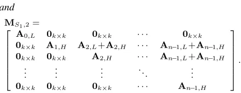
Proposition 1. The Mastrovito matrix MS1 can be con-structed as
MS1 =MS1,1+MS1,2,
where
MS1,1=
A0,L+A0,H A1,L+A1,H · · · An−1,L+An−1,H .
.
. ... . .. ...
A0,L+A0,H A1,L+A1,H · · · An−1,L+An−1,H
and
MS1,2=
A0,L 0k×k 0k×k · · · 0k×k
0k×k A1,H A2,L+A2,H · · · An−1,L+An−1,H
0k×k 0k×k A2,H · · · An−1,L+An−1,H .
.
. ... ... . .. ...
0k×k 0k×k 0k×k · · · An−1,H
.
Proof. The proof is the same as the proof of Lemma 2. We directly get this conclusion by substitutingAbyAS1.
It is noted that there are some overlapped terms between
MS1,1 and MS1,2. By adding these two matrices together,
we can obtain the explicit form ofMS1, which is shown in
(7). Moreover, the matrix-vector multiplicationS1=MS1·b
can be computed according to the strategy used in [25] and overlapped terms are considered reusing to save more logic gates.
1) Detailed computation ofS1modulof(x).
(i) Perform2nrow-vector products
A0,L∗b0,A0,H∗b0,A1,L∗b1,A1,H∗b1,
· · · An−1,L∗bn−1,An−1,H∗bn−1,
(8)
in parallel. The symbol “*” represent only row-vector product related to Ai,L (or Ai,H) and bi, i = 0,1,· · ·, n−1. For instance, A0,H ∗ b0 represents
computing the products
[A0,H(i,1)·b0,· · ·,A0,H(i, k)·bk−1],
fori= 1,2,· · ·, kin parallel. (ii) Compute
A0,Lb0+A0,Hb0,· · ·,An−1,Lbn−1+An−1,Hbn−1
using binary XOR trees in parallel. Meanwhile,
A0,Hb0,A1,Lb1,· · ·,An−1,Lbn−1 are computed
us-ingsub-expression sharingtechnique.
(iii) Sum up all thenentries of each row using binary XOR tree to obtain the final result.
Remark.It is clear that the row-vector products in (8) contain all the possible row-vector products in (7). Only nk2 AND
gates are required to compute these expressions.
In addition,Ai,Lbi+Ai,Hbi,(i= 0,· · · , n−1)contain
all the terms of Ai,Lbi or Ai,Hbi. These expressions can
be computed in parallel and more logic gates can be saved using sub-expression sharing for binary tree. Such an ap-proach has already been studied in [24]. The authors have shown that if two binary XOR trees sharetcommon items, only t −W(t) XOR gates can be saved, where W(t) is the Hamming weight of t. It is easy to check that the j -th row (j = 1,2,· · · , k) of Ai,Lbi shares j terms with Ai,Lbi+Ai,Lbi fori = 1,2,· · · , n−1. Meanwhile, the
j-th row ofAi,Lbi includesj terms and originally requires
j−1XOR gates for binary XOR tree. Minus the saved XOR gates, we can see that number of required XOR actually is j−1−(j−W(j)) =W(j)−1. Specifically, thek-th row of
TABLE 1. Space and time complexities ofS1modf(x)
Operation # AND #XOR Delay
Ai,L∗bi,Ai,H∗bi nk2 - TA
Ai,Lbi+Ai,Hbi
- n(k2−k)
dlog2keTX
(i= 0,1,· · ·, n−1)
A0,Hb0,Ai,Lbi
- n
Pk−1
i=1W(i) (i= 1,2,· · ·, n−1) +n−nk
S1
- m+kW(n−2)
dlog2neTX +kPn−2
i=0W(i)
Ai,Lbiis identical to that ofAi,Lbi+Ai,Lbi, no XOR gates
is needed here. Based on similar approach, we can calculate the real number of XOR gates for thej-th row ofA0,Hb0is
W(k−j)−1forj = 1,2,· · ·, k−1.
Table 1 summarizes the space and time complexity of S1modf(x) for all the steps. One can notice that after
calculation of the row-vector products in (8), each row of
Ai,L ∗bi+Ai,H ∗bi consists of kterms. Thus, the inner
product ofAi,Lbi+Ai,Hbiwill be obtained using a binary
XOR tree with a delay of dlog2keTX. Finally, we have to
perform additions among the nentries to obtain the coeffi-cient vector with respect toS1. More partial additions can be
saved using the same sub-expression sharing. For simplicity, we put the details to the appendix A.
2) An example ofS1modf(x)
Firstly we have an irreducible 4-spaced trinomialx4+x+ 1
overF2. Then, we can construct another irreducible 4-spaced
trinomial of higher degree according to Lemma 1, i.e.,x12+
x3+ 1.
Consider the field multiplication using SPB representa-tion over GF(212) defined by the previous trinomial. We
have the SPB parameter k = 3 and SPB is defined as {x−3, x−2,· · · , x7, x8}. Assume thatA=P11
i=0aix i−3and
B = P11i=0bixi−3 are two elements inGF(212).A, B are
partitioned as
A=A3x6+A2x3+A1+A0x−3,
B=B3x6+B2x3+B1+B0x−3,
whereAi = a2+3ix2+a1+3ix+a0+3i, Bi = b2+3ix2+
b1+3ix+b0+3i, fori= 0,1,2,3.
Based on equation (2) and previous description, it is obvi-ously thatAB=S1+S2and the explicit form ofS1andS2
are as follows:
S1=A3B3hx6+A2B2hx3+A1B1h+A0B0hx−3,
S1modf(x) =MS1·b=
A0,H A1,L+A1,H A2,L+A2,H · · · An−2,L+An−2,H An−1,L+An−1,H
A0,L+A0,H A1,L 0k×k · · · 0k×k 0k×k
A0,L+A0,H A1,L+A1,H A2,L · · · 0k×k 0k×k
..
. ... ... . .. ... ...
A0,L+A0,H A1,L+A1,H A2,L+A2,H · · · An−2,L 0k×k
A0,L+A0,H A1,L+A1,H A2,L+A2,H · · · An−2,L+An−2,H An−1,L
· b0 b1 .. .
bn−2
bn−1
. (7)
whereh(x) =x6+x3+1+x−3andE
s,t= (As+At)(Bs+
Bt)for3≥s > t≥0. Let
Ai,L=
a3i+0 0 0
a3i+1 a3i+0 0
a3i+2 a3i+1 a3i+0
,
and
Ai,H=
0 a3i+2 a3i+1 0 0 a3i+2
0 0 0
.
Accordingly, it is easy to compute the matricesAS1,MS1,1
andMS1,2, which are presented in the appendix. The
Mas-trovito matrix related toS1modf(x)is
A0,H A1,L+A1,H A2,L+A2,H A3,L+A3H
A0,L+A0,H A1,L 0k×k 0k×k
A0,L+A0,H A1,L+A1,H A2,L 0k×k
A0,L+A0,H A1,L+A1,H A2,L+A2,H A3,L
=
0 a2 a1 a3 a5 a4 a6 a8 a7 a9 a11 a10
0 0 a2 a4 a3 a5 a7 a6 a8 a10 a9 a11
0 0 0 a5 a4 a3 a8 a7 a6 a11 a10 a9
a0 a2 a1 a3 0 0 0 0 0 0 0 0
a1 a0 a2 a4 a3 0 0 0 0 0 0 0
a2 a1 a0 a5 a4 a3 0 0 0 0 0 0
a0 a2 a1 a3 a5 a4 a6 0 0 0 0 0
a1 a0 a2 a4 a3 a5 a7 a6 0 0 0 0
a2 a1 a0 a5 a4 a3 a8 a7 a6 0 0 0
a0 a2 a1 a3 a5 a4 a6 a8 a7 a9 0 0
a1 a0 a2 a4 a3 a5 a7 a6 a8 a10 a9 0
a2 a1 a0 a5 a4 a3 a8 a7 a6 a11 a10 a9 .
Therefore, one can check that the exact number of logic gates requried by every step ofS1modf(x):
• Computation of A0,L ∗ b0,A0,H ∗ b0,· · · ,A3,L ∗ b3,A3,H∗b3requires36AND gates with oneTAgate
delay.
• Computation of A0,Lb0 +A0,Hb0,· · ·,A3,Lb3 + A3,Hb3 costs 24 XOR gates in all. Meanwhile,
no XOR gates are needed for the computation of A0,Hb0,A1,Lb1,A2,Lb2,A3,Lb3 using
sub-expression sharing, as the binary XOR tree for these expressions can be embedded into those of Ai,Lbi+ Ai,Hbi for i = 0,1,2,3. These operations requires 2TX delay in parallel.
• The final additions among 4entries of each row costs 21 XOR gates using the trick presented in the appendix, which cost another2TXdelay in parallel.
As a result, the calculation of MS1,1·btotally requires 36
AND gates and 45 XOR gates, withTA+ 4TX gate delay.
This result meets the complexity formulae shown in Table 1.
B. COMPUTATION OFS2MODULOXN K+XK+ 1 We then consider the computation ofS2modf(x)in details.
Note that
S2= 2n−3
X
i=1
X
s+t=i, n>s>t≥0
Es,t
xik−2k
andEs,t = (As+At)(Bs+Bt),(n > s > t≥0)consist
of k bits. Each of these expressions can be recognized as a small matrix-vector multiplication. LetPk−1
i=0 u (s,t) i xi and Pk−1
i=0 v (s,t)
i xi denote the result ofAs+AtandBs+Bt,
respectively. We haveEs,t = Us,t·vs,t, whereUs,tis the
product matrix constructed from Pk−1 i=0 u
(s,t)
i xi andvs,t is
the coefficient vector[v0(s,t), v1(s,t),· · · , v(ks,t−1)]T, i.e.,
Es,t=Us,t·vs,t=
u(0s,t) 0 · · · 0 0
u(1s,t) u(0s,t) · · · 0 0
..
. ... . .. ... ... uk(s,t−2) u(ks,t−3) · · · u(0s,t) 0
uk(s,t−1) uk(s,t−2) · · · u(1s,t) u(0s,t)
0 u(ks,t−1) · · · u(2s,t) u(1s,t) ..
. ... . .. ... ...
0 0 · · · uk(s,t−1) u(ks,t−2)
0 0 · · · 0 u(ks,t−1)
·
v0(s,t) v1(s,t)
.. . vk(s,t−2) vk(s,t−1)
. (9)
It is noted that these matrix-vector multiplications are in-dependent and thus can be implemented in parallel. However, S2contains n2
different expressions in all, each of which has a different degree. In order to simplify the reduction process, we first classify these expressions into several categories, where the expressions in the same category can constitute a bigger matrix-vector multiplication. Then we can perform a reduction with each category. In addition, the classification has already been studied in [23]. Here, we can utilize the result directly. Let
S(n) =S2·x2k = 2n−3
X
i=1
X
s+t=i, n>s>t≥0
Es,t
xik.
The classification lemma is as follows:
Lemma 3. [23] S(n) can be expressed as the plus of
g1x(2λ−1)k, g2x(2λ−3)k,· · · , gλxk forλ= n2 (nis even) or
λ= n−21 (nis odd), where
g1=C (1)
n−2x(n−2)k+C (1)
n−3x(n−3)k+· · ·+C (1) 0 ,
g2=C (2)
n−2x(n−2)k+C (2)
n−3x(n−3)k+· · ·+C (2) 0 , ..
.
gn 2 =C
(n 2)
n−2x(n−2)k+C (n
2)
n−3x(n−3)k+· · ·+C (n
2) 0 , or
g1=C (1)
n−1x(n−1)k+C (1)
n−2x(n−2)k+· · ·+C (1) 0 ,
g2=C (2)
n−1x(n−1)k+C (2)
n−2x(n−2)k+· · ·+C (2) 0 , ..
.
gn−1 2 =C
(n−12 )
n−1 x(n−1)k+C (n−12 )
n−2 x(n−2)k+· · ·+C (n−12 )
0 ,
whereCj(i)∈ {Es,t}, n > s > t≥0.
Proof. See section 3.2 in [23].
Based on the above lemma, it is obvious thatS2can be
par-titioned intoλparts and all these parts are independent. More explicitly,S2 = g1x(2λ−3)k+g2x(2λ−5)k +· · ·+gλx−k.
Obviously, g1, g2,· · ·, gλ contain all the nonzero terms of
S2, where the number of such terms equals(n−2)k+ 2k− 2 + 1 = m−1terms ifnis even or(n−1)k+ 2k−2 + 1 = m+k−1 if n is odd. We can first compute these expressions in parallel, then, perform reductions related to g1x(2λ−3)k, g2x(2λ−5)k,· · · , gλx−k.
1) Detailed computation ofS2modf(x)
(i) Perform bitwise additionAs+At, Bs+Bt,(n > s >
t≥0)in parallel.
(ii) Perform n2matrix-vector bitwise multiplications, i.e,
Es,t=Us,t∗vs,tin parallel.
(iii) Classify these n2matricesEs,tintoλparts according
to Lemma 3 and constitute the small matrices of the same category intoλbig matricesEg1,· · ·,Egλ, which
correspond tog1, g2,· · ·, gλ.
(iv) Add all the entries of the same row in Eg1,· · ·,Egλ
using binary XOR tree, and obtain the coefficients of g1, g2,· · · , gλ.
(v) Perform reduction forg1x(2λ−3)k, g2x(2λ−5)k,· · ·, gλx−k
modulof(x)using (4).
(vi) Add all these results binary XOR tree to obtain the S2modf(x).
Remark. According to (9), it is clear that after performing bitwise multiplication, Es,t are all(2k−1)×k matrices.
When we classify these matrices and constitute them to λ big matrices, one can check that the number of entries for each row of Eg1,· · ·,Egλ is equal to k. Thus, the
coeffi-cients of g1, g2,· · · , gλ will be obtained with dlog2keTX
delay. Whereafter, we can perform the modular reduction for g1x(2λ−3)k, g2x(2λ−5)k,· · · , gλx−k. Such reductions also
rely on equation (4). We have following observations for the
computation ofS2modf(x).
Observation 3.2.1 To compute g1x(2λ−3)k, g2x(2λ−5)k, · · · , gλx−k modulo f(x), we only need to reduce these
expressions at most once.
Proof. Apparently, the minimal and maximal degrees of the terms ing1x(2λ−3)k, g2x(2λ−5)k,· · ·, gλx−kare−kand 2m−3k−2, respectively. Apply reducing formulae of (4), we have
xm−k=x0+x−k, xm−k+1=x1+x−k+1,
.. .
x2m−3k−2=xm−2k−2+xm−3k−2.
The exponents ofxin the right side now are all in the range
[−k, m−k−1], no further reduction is needed.
Observation 3.2.2When the modular reduction and addition are combined, Step (v) and (vi) can be calculated with at most dlog2neTXdelay.
Proof. We knowg1x(2λ−3)k, g2x(2λ−5)k,· · ·, gλx−k
modu-lof(x)only need to reduced once. But,gicontains different
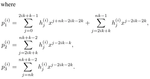
number of nonzero terms according to the parity ofn, which lead to different reduction formulations. For simplicity, we only consider the case of odd n here and put the analysis about other case in Appendix.
If n is odd, we haveλ = n−21, and the degree of gi is
nk+k−2. Letgi=P nk+k−2
j=0 h
(i) j x
j. Then,
gix(n−2i−2)k =
2ik+k−1 X
j=0
h(ji)xj+(n−2i−2)k+
nk−1 X
j=2ik+k
h(ji)xj+(n−2i−2)k+ nk+k−2
X
j=nk
h(ji)xj+(n−2i−2)k,
for i = 1,2,· · ·,n−21. When we reduce above expression modulof(x) = xnk+xk+ 1, only two parts are needed to
be reduced. Then,
nk−1
X
j=2ik+k
h(ji)xj+(n−2i−2)k= nk−1
X
j=2ik+k
h(ji)(xj−2ik−2k+xj−2ik−k),
nk+k−2
X
j=nk h(ji)x
j+(n−2i−2)k =
nk+k−2
X
j=nk h(ji)(x
j−2ik−2k
+xj−2ik−k).
By combining non-overlapped parts of above expressions, the result ofgix(n−2i−2)kmodf(x)is given by
gix(n−2i−2)kmodf(x) =p (i) 1 (x) +p
(i) 2 (x) +p
where
p(1i)=
2ik+k−1 X
j=0
h(ji)xj+nk−2ik−2k+ nk−1
X
j=2ik+k
h(ji)xj−2ik−2k,
p(2i)= nk+k−2
X
j=2ik+k
h(ji)xj−2ik−k,
p(3i)= nk+k−2
X
j=nk
h(ji)xj−2ik−2k.
Moreover, it is noted that the term degrees ofp(3i)are in the range[nk−2ik−2k, nk−2ik−k−2]. One can check that these ranges are[−k,−2],[k,2k−2],· · · ,[(n−4)k,(n−
3)k−2]. Therefore, there is no overlapped term among all thep(3i), which cost no XOR gates to add them up. Denoted byrthe addition ofp(1)3 , p(2)3 ,· · · , p(
n−1 2 )
3 .
Consequently, to obtain S2modf(x), we only need to
add p(1)1 , p(1)2 ,· · ·, p(
n−1 2 ) 1 , p
(n−12 )
2 and r in parallel, which
cost dlog2ne XOR gate delay. We directly conclude the observation.
We next analyze the space and time complexity related to S2. Firstly, 2k· n2
= (n2 −n)k XOR gates are needed for pre-computation of As+At andBs +Bt,(n > t >
s ≥0)in Step (i), which cost oneTX in parallel. Then, the n
2
matrix-vector bitwise multiplications in Step (ii) costk2· n
2
= (n2−n)k2/2AND gates withT
Agate delay.
The classification in Step (iii) does not cost any logic gates. Step (iv) includes adding all the entries of the same row in Eg1,· · ·,Egλ. Since these matrices are determined
byg1, g2,· · ·, gλ, the required XOR gates varies according
to parity ofn. Ifnis even, each ofg1, g2,· · ·, gn
2 consists of
n−1sub-polynomials. That is to say,Egi,(i= 1,2,· · ·, n 2
corresponds a combination of n −1 matrices Es,t. Thus
the coefficient computation for each gi costs nk2 −k2 −
m + 1 XOR gates with dlog2keTX delay. If n is odd,
g1, g2,· · · , gn−1
2 consists of
nsub-polynomials. Similarly, it costsnk2−k−m+1XOR gates for eachgiwithdlog2keTX
delay.
Step (v) and (vi) follow the description in Observation 3.2.2. We only addn (orn−1) vectors together to obtain S2modf(x). The space and time complexity for all the
steps is stated in Table 2.
2) An example ofS2modf(x)
To illustrate our classification and reduction strategy, we give a small example here. ConsiderS2presented in former
example. According to Lemma 3,S1can be rewritten as
S1=g1x3+g2x−3,
where g1 = E3,2x6 +E3,1x3 +E3,0, g2 = E2,1x6 +
E2,0x3+E1,0. LetAs+At= P2
i=0u
(s,t)xiandB
s+Bt=
TABLE 2. Space and time complexities ofS2modf(x)
Operation # AND #XOR Time delay
As+At - (n
2−n)k
2 T
X Bs+Bt - (n
2−n)k 2
Us,t∗vs,t (n
2−n)k2
2 - TA
Step (iv) - m2−km2−mn+n dlog2keTX
Step (v)(vi) - 3nm4 −3m
2 −
n
2+1 dlog2(n−1)eTX
Step (iv)∗ - m2−km−mn2 +k+n−1 dlog2keTX
Step (v)(vi)∗ - 3nm4 −3m
2 −
k
4−n+1 dlog2neTX
* represents the case of oddn.
P2
i=0v(s,t)xifor3≥s > t≥0. The explicit form ofEg1is
given by
Eg1 =
u(30,0)v(30,0) 0 0
u(31,0)v(30,0) u(30,0)v(31,0) 0
u(32,0)v(30,0) u(31,0)v(31,0) u(30,0)v2(3,0) u(30,1)v(30,1) u(32,0)v(31,0) u(31,0)v2(3,0) u(31,1)v(30,1) u(30,1)v(31,1) u(32,0)v2(3,0) u(32,1)v(30,1) u(31,1)v(31,1) u(30,1)v2(3,1) u(30,2)v(30,2) u(32,1)v(31,1) u(31,1)v2(3,1) u(31,2)v(30,2) u(30,2)v(31,2) u(32,1)v2(3,1) u(32,2)v(30,2) u(31,2)v(31,2) u(30,2)v2(3,2)
0 u(32,2)v1(3,2) u(31,2)v2(3,2)
0 0 u(32,2)v2(3,2)
0 0 0
.
The organization of Eg2 is almost the same as Eg1. It is
easy to see that the computation of g1, g2 in Step (iv) cost
32 XOR gates with 2TX delay. In addition, 17 more XOR
gates are needed as well for Step (v) and (vi) with2TXdelay.
Combined with the number of logic gates required in Step (i), (ii), it totally requires 54 AND and 85 XOR gates for S2modf(x), withTA+ 5TXdelay.
C. THEORETIC COMPLEXITY
After the computation ofS1andS2modulof(x), otherm
X-OR gates are needed to add two results together. From Table 1 and 2, it is clear that the delay ofS2modf(x)cost one more
TX thanS1modf(x). Thus, in parallel implementation of
S1, S2 modulo f(x), the delay is TA + (1 +dlog2ke+ dlog2ne)TX (or TA+ (1 +dlog2ke+dlog2(n−1)e)TX
for evenn). Plus one moreTXthat cost in the final addition,
we obtain the time complexity of our proposed architecture as
Time delay=TA+ (2 +dlog2ke+dlog2ne)TX.
The space complexity is
# AND= m2
2 +
mk
2 , # XOR=m2
2 +
mk
2 + 5mn
4 +n
Pk−1
i=1W(i) +n
+kPn−2
i=1 W(i) +kW(n−2)− 5m
2 + 1, # XOR∗=m2
2 +
mk
2 + 5mn
4 +n
Pk−1
i=1 W(i)+
n
2
+k4+kPn−2
i=1 W(i) +kW(n−2)− 5m
2 + 1 2.
(10)
The symbol “*” represent the case of oddn. The formulation for the number of XOR varies according to the parity of n. We note that these formulae contain sums of hamming weights related to k−1 or n−2. In fact, the expression
Pδ
i=0W(i)can be roughly written as δ
2log2δ[22], whereδ
is a nonzero integer. Thus, the hamming weight formulations related tonroughly equalO(mlog2n), while the formula-tions related to k are roughly equal to O(mlog2k). Omit the linear parts, the number of required XOR gates can be rewritten as:
m2 2 +
mk
2 +
5mn
4 +O(mlog2k) +O(mlog2n). (11)
The above formula reveals the lower bound of the space complexity of our proposal. Based on (10) and (11), it is obvious that with the increase of the parametern, the number of required AND gates is decreasing. If n = m, #AND achieves its lower bound, i.e., m22+m. But at this time, the number of required XOR gates is more than 7m42. Therefore, the optimal parameter n should be the one that minimizes both the number of XOR and AND gates. We combine the two formulations with respect to #AND and #XOR, define a function:
M(n) =m2+mk+5mn 4
1.
Please note thatm=nk. Obviously,M(n) =m2+m2
n +
5mn 4 . When
m2
n =
5mn
4 , namely,n= 2( m
5)
1/2, we obtain the
minimal value ofM(n), which indicate the best asymptotic space complexity of our proposal. In this case, we see thatk is almost equal ton. The space complexity is
# AND=m22 +
√
5m3/2 4 ,
# XOR=m2 2 +
3√5m3/2
4 +O(mlog2k).
Figure 1 shows the space complexity tendency with the increase of n. It is clear that n could not always increase. Combined with the lowest asymptotic space complexity analysis, we can see that our proposal is more suitable for xnk+xk+ 1, wherenis smaller thank.
1Here, we assume that the XOR and AND consist of the same number of transistors. In practical application, one can modify this function by multiplying different weight factors.
n
#XOR #AND
FIGURE 1. Space complexity tendency with increase ofn.
IV. SPEEDUP STRATEGY
As shown in previous section, the time delay of our proposal isTA+ (2 +dlog2ke+dlog2ne)TX. Since
dlog2ke+dlog2ne ≤ dlog2me+ 1,
the upper bound of the delay isTA+ (3 +dlog2me)TX. This
result is worse than the multiplier using classic Karatsuba algorithm. The main reason is the delay ofS2is bigger than
that of S1. Indeed, we can add the intermediate values in
advance during the computation process ofS1, S2to speed up
the whole architecture. For better comprehension, we define some additional notations.
• qS1,0,qS1,1,· · ·,qS1,n−1represent the coordinate
vec-tors ofMS1(:, i∼ik)·bi+1in (7) after the computation
ofAi,Lbi+Ai,Hbi, i= 0,1,· · ·, n−1.
• qS2,0,qS2,1,· · ·,qS2,n−1represent the coordinate
vec-tors corresponding to the polynomials p(1)1 , p(1)2 ,· · ·, p(
n−1 2 ) 1 , p
(n−12 ) 2 and r
2after we compute the entries
additions of Step (v). For example,
qS1,0= [A0,Hb0,(A0,L+A0,H)b0,· · ·,(A0,L+A0,H)b0]
T ,
qS2,0=
h
h(1)3k,· · ·, h(1)nk−1, h (1) 0 ,· · ·, h
(1) 3k−1]
T .
According to Table 1 and 2, it is easy to see that the compu-tation ofqS1,0,qS1,1,· · ·,qS1,n−1costTA+dlog2keTX, while
qS2,0,qS2,1,· · ·,qS2,n−1costTA+ (1 +dlog2ke)TX.
Our speedup strategy is adding these vectorqS1,iandqS2,i di-rectly before completingS1andS2. Since the computation ofqS2,i cost one moreTX thanqS1,i, we can perform one more addition for each two vectors, i.e.,qS1,i+qS1,i+1fori= 0,2,· · ·, n−2 (or i = 0,2,· · ·, n −3 if n is odd). After this addition, we obtaindn
2ecolumn vectors. Plusn(orn−1) coordinate vectors
qS2,0,qS2,1,· · ·,qS2,n−1, there are at mostd 3n
2 evectors need to be added, which requires only dlog2d3n
2eeTX. The computation sequence of our architecture is arranged as shown in Fig.1.
As a result, the whole time delay is
TA+ (1 +dlog2ke+dlog2d
3n 2 ee)TX.
2Ifnis even, there only n−1 coordinate vectors corresponding to
p(1)1 , p(1)2 ,· · ·, p(
n 2−1) 1 ,p
(n2−1) 2 , gn2x
A
s+A
tB
s+B
tA
i,L*
b
i,
A
i,H*
b
iA
i,Lb
i+A
i,Hb
iU
s,t*
v
s,tTX
log2k
TXTX
log2k
TA
TA
q
s2,1,...,
q
s2,n-1q
,0+
q
,1q
,2+
q
,3. . .
q
,n-2+
q
,n-1 1s s1
1
s s1
1
s
1
s
TA
Final addition for at most 3n/2 vectors
TX
2 3 log2
n
S
2:
S
1:
n-1 vectors
n/2 vectors
FIGURE 2. Speedup strategy related to our architecture.
Furthermore, based on Lemma 3 of [11], we have1+dlog2d 3n
2 ee= dlog23ne. Thus, the time delay formulation can be simplified as
TA+ (dlog2ke+dlog23ne)TX.
V. COMPARISON AND DISCUSSION
According to the descriptions in the previous section, it is clear that the time delay of our proposal using speedup strategy is
TA+ (dlog2ke+dlog23ne)TX. However, it is especially attractive
if
dlog2ke+dlog23ne=dlog23n·ke=dlog23me. (12)
At this time, the corresponding time delay isTA+dlog23me)TX,
which approximately equals the fastest 2-term Karatsuba based multiplier [24]. In fact, we have checked all the irreduciblexnk+ xk+ 1, k >1of degreem=nk∈[100,1023]overF2, and found about54%such trinomials satisfy (12), and the rest of them requires at most oneTXthan than the fastest Karatsuba multiplier so far.
Table 3 gives a comparison of different implementations of bit-parallel multipliers in the fields generated by trinomialsxm+xk+ 1, m =nk. More explicitly, we omit the expressionO(mlog2n) in (11), asnis usually smaller thankshown in Section 3.3. Based on this table, it is easy to see that our proposal has better space complexity while maintain relatively low time complexity. The best of our result only costs about m22 +O(m3/2)
circuit gates compared with the previous architectures without using a divide-and-conquer algorithm. On the other hand, the time complexity of the proposed multiplier is very closed to the fastest result utilizing classic Karatsuba algorithm.
.
VI. CONCLUSION
In this paper, we investigate the application of an-term Karatsuba algorithm and develop a new type of bit-parallel multiplier for a class of irreducible trinomials. The proposed architecture shows that specific type of trinomials combined with Karatsuba algorithm variations can reduce the space complexity further compared with classic Karatsuba multipliers. We next work on the construction of
n-term Karatsuba multiplier for general trinomials. .
TABLE 4. Saved XOR gates about the entries addition
Matrix rows Overlapped terms Saved #XOR
1∼k (n−2)k ((n−2)−W(n−2))k
k+ 1∼2k k 1−W(1))k
2k+ 1∼3k 2k (2−W(2))k
..
. ... ...
(n−2)k+ 1∼
(n−2)k ((n−2)−W(n−2))k (n−1)k
(n−1)k+ 1∼m nk (n−1)k
APPENDIX A THE SUB-EXPRESSION SHARING FOR ENTRIES ADDITION INS1
LetPidenote the coordinate vector ofAi,Lbi+Ai,HbiandP0i
denote the coordinate vector of Ai,Lbi (orAi,Hbi fori = 0).
Clearly, bothPiandP0iarek×1vectors. Therefore, (7) can be
rewritten as:
MS1·b=
P00 P1 P2 · · · Pn−2 Pn−1
P0 P01 0 · · · 0 0
P0 P1 P02 · · · 0 0
..
. ... ... . .. ... ...
P0 P1 P2 · · · P0n−2 0
P0 P1 P2 · · · Pn−2 P0n−1
.
So we only need to compute entries additions fork intermediate coordinate vectors
P0+P1+· · ·+Pn−2+P0n−1 (13)
and all the entries additions can be computed through reusing these values. Table 4 indicates the overlapped values and the number of saved XOR gates.
Note that the additions between these vectors without sub-expression sharingrequire2(n−1)k−kPn−2
i=1 iXOR gates. By
TABLE 3. Comparison of bit-parallel Multipliers forGF(2m)generated withxm+xk+ 1,(m=nk)
Multiplier # AND #XOR Time delay
Sunar [7] m2 m2−1 TA+ (2 +dlog2me)TX
Wu [16] m2 m2−1 TA+ (2 +dlog2me)TX
Wu [17] m2 m2−1 TA+ (2 +dlog2me)TX
Fan [13] m2 m2−1 TA+dlog2(2n−1)keTX
Elia [14] 3m2
4
3m2
4 + 13m
3 − 23
4 TA+ (3 +dlog2me)TX
Négre [27] m2 23m2
18 − 3m
2 TA+dlog2(2n−1)keTX
Fan [11] Type-A m2−m
3 m 2−m
3 TA+dlog2(max((3n−3)k,(2n−2)k+2
v ))eTX
Type-B m2−m
3 m 2−2m
3 +
m
3 ·W(
m
3) TA+dlog2((3n−3)k−1)eTX
Li [24] 3m2+24m−1 3m42+m
2+O(mlog2m) TA+ (1 +dlog2(2n−1)ke)TX
Li [25] (x3k+xk+ 1
) 2m32 2m32 +7m
3 −1 TA+dlog2 8m
3 e)TX This paper m22 +mk
2 m2 2 + mk 2 + 5mn
4 +O(mlog2k) TA+ (dlog2ke+dlog23ne)TX
where2v−1
<m
3 ≤2
v
andW(∗)is the hamming weight of the number *
subtracting the number of saved XOR gates, the number of required XOR gates actually is
m+k n−2
X
i=1
W(i) +kW(n−2).
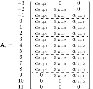
APPENDIX B RELATED MATRICES IN EXAMPLE 3.1
As we know the form ofAi,L andAi,H, it is easy to obtain the
explicit formulae with respect toAi(i= 0,1,2,3), andAS1.
For the size of the above matrix, we do not present the line number in the left side. One should note that the rows of AS1 correspond the term degree [-6, 17].
Ai=
−3 −2 −1 0 1 2 3 4 5 6 7 8 9 10 11
a3i+0 0 0
a3i+1 a3i+0 0
a3i+2 a3i+1 a3i+0
a3i+0 a3i+2 a3i+1
a3i+1 a3i+0 a3i+2
a3i+2 a3i+1 a3i+0
a3i+0 a3i+2 a3i+1
a3i+1 a3i+0 a3i+2
a3i+2 a3i+1 a3i+0
a3i+0 a3i+2 a3i+1
a3i+1 a3i+0 a3i+2
a3i+2 a3i+1 a3i+0
0 a3i+2 a3i+1
0 0 a3i+2
0 0 0
, and
AS1=
a0 0 0 0 0 0 0 0 0 0 0 0
a1 a0 0 0 0 0 0 0 0 0 0 0
a2 a1 a0 0 0 0 0 0 0 0 0 0
a0 a2 a1 a3 0 0 0 0 0 0 0 0
a1 a0 a2 a4 a3 0 0 0 0 0 0 0
a2 a1 a0 a5 a4 a3 0 0 0 0 0 0
a0 a2 a1 a3 a5 a4 a6 0 0 0 0 0
a1 a0 a2 a4 a3 a5 a7 a6 0 0 0 0
a2 a1 a0 a5 a4 a3 a8 a7 a6 0 0 0
a0 a2 a1 a3 a5 a4 a6 a8 a7 a9 0 0
a1 a0 a2 a4 a3 a5 a7 a6 a8 a10 a9 0
a2 a1 a0 a5 a4 a3 a8 a7 a6 a11 a10 a9
0 a2 a1 a3 a5 a4 a6 a8 a7 a9 a11 a10
0 0 a2 a4 a3 a5 a7 a6 a8 a10 a9 a11
0 0 0 a5 a4 a3 a8 a7 a6 a11 a10 a9
0 0 0 0 a5 a4 a6 a8 a7 a9 a11 a10
0 0 0 0 0 a5 a7 a6 a8 a10 a9 a11
0 0 0 0 0 0 a8 a7 a6 a11 a10 a9
0 0 0 0 0 0 0 a8 a7 a9 a11 a10
0 0 0 0 0 0 0 0 a8 a10 a9 a11
0 0 0 0 0 0 0 0 0 a11 a10 a9
0 0 0 0 0 0 0 0 0 0 a11 a10
0 0 0 0 0 0 0 0 0 0 0 a11
0 0 0 0 0 0 0 0 0 0 0 0
.
After reduction process, the explicit form ofMS1,1andMS1,2 are presented as follows:
MS1,1=
a0 a2 a1 a3 a5 a4 a6 a8 a7 a9 a11 a10
a1 a0 a2 a4 a3 a5 a7 a6 a8 a10 a9 a11
a2 a1 a0 a5 a4 a3 a8 a7 a6 a11 a10 a9
a0 a2 a1 a3 a5 a4 a6 a8 a7 a9 a11 a10
a1 a0 a2 a4 a3 a5 a7 a6 a8 a10 a9 a11
a2 a1 a0 a5 a4 a3 a8 a7 a6 a11 a10 a9
a0 a2 a1 a3 a5 a4 a6 a8 a7 a9 a11 a10
a1 a0 a2 a4 a3 a5 a7 a6 a8 a10 a9 a11
a2 a1 a0 a5 a4 a3 a8 a7 a6 a11 a10 a9
a0 a2 a1 a3 a5 a4 a6 a8 a7 a9 a11 a10
a1 a0 a2 a4 a3 a5 a7 a6 a8 a10 a9 a11
MS1,2=
a0 0 0 0 0 0 0 0 0 0 0 0
a1 a0 0 0 0 0 0 0 0 0 0 0
a2 a1 a0 0 0 0 0 0 0 0 0 0
0 0 0 0 a5 a4 a6 a8 a7 a9 a11 a10
0 0 0 0 0 a5 a7 a6 a8 a10 a9 a11
0 0 0 0 0 0 a8 a7 a6 a11 a10 a9
0 0 0 0 0 0 0 a8 a7 a9 a11 a10
0 0 0 0 0 0 0 0 a8 a10 a9 a11
0 0 0 0 0 0 0 0 0 a11 a10 a9
0 0 0 0 0 0 0 0 0 0 a11 a10
0 0 0 0 0 0 0 0 0 0 0 a11
0 0 0 0 0 0 0 0 0 0 0 0
.
APPENDIX C PROOF OF OBSERVATION FOR EVENN
Ifnis even, we haveλ= n
2, and the degree ofgiisnk−2. Let
gi=Pnk
−2
j=0 h (i)
j x j. Then
gix(n−2i−1)k=
2ik−1
X
j=0
h(ji)x
j+(n−2i−1)k +
nk−2
X
j=2ik h(ji)x
j+(n−2i−1)k ,
fori= 1,2,· · ·,n
2 −1. Similar with case of oddn, only one part of the above expression needs reduction byf(x). We have
nk−2
X
j=2ik
h(ji)xj+(n−2i−1)k= nk−2
X
j=2ik
h(ji)(xj−2ik−k+xj−2ik).
We note that ifi = n
2, all the term degrees ofgn2x −k
are in the range[−k, nk−k−1]. No further reduction is needed.
By combining non-overlapped parts of above expressions, the result ofgix(n−2i−1)kmodf(x)is given by
gn 2x
−k
modf(x) =gn 2x
−k
gix(n
−2i−1)k
modf(x) =p(1i)(x) +p(2i)(x),
where
p(1i)=
2ik−1
X
j=0
h(ji)xj+nk−2ik−k+ nk−1
X
j=2ik
h(ji)xj−2ik−k,
p(2i)= nk−2
X
j=2ik
h(ji)xj−2ik,
for i = 1,2,· · ·,n2 − 1. Therefore, in this case, to obtain
S2modf(x), we only need to addp(1)1 , p (1) 2 ,· · ·, p
(n 2−1) 1 , p
(n 2−1) 2 andgn
2x −k
in parallel, which costdlog2(n−1)eXOR gate delay.
REFERENCES
[1] A. J. Menezes, I. F. Blake, X. Gao, R. C. Mullin, S. A. Vanstone and T. Yaghoobian, Applications of Finite Fields. Kluwer Academic, Norwell, Massachusetts, USA, 1993.
[2] R. Lidl and H. Niederreiter, Finite Fields. Cambridge University Press, New York, NY, USA, 1996.
[3] I. Blake, G. Seroussi and N. Smart, Elliptic Curves in Cryptography. Lond. Math. Soc. Lect. Note Ser., vol. 265, Cambridge University Press, 1999. [4] A. Karatsuba and Yu. Ofman. "Multiplication of Multidigit Numbers on
Automata," Soviet Physics-Doklady (English translation), vol. 7, no. 7, pp. 595–596, 1963.
[5] H. Fan and M. A. Hasan, “Fast bit parallel-shifted polynomial basis multipliers inGF(2n),” Circuits and Systems I: Regular Papers, IEEE Transactions on, vol. 53, no. 12, pp. 2606–2615, Dec 2006.
[6] H. Fan and M. A. Hasan, “A survey of some recent bit-parallel multipliers,” Finite Fields and Their Applications, vol. 32, pp. 5–43, 2015.
[7] B. Sunar and Ç. K. Koç, “Mastrovito multiplier for all trinomials,” IEEE Trans. Comput., vol. 48,no. 5, pp. 522–527, 1999.
[8] A. Weimerskirch, and C. Paar, "Generalizations of the Karatsuba Algo-rithm for Efficient Implementations," Cryptology ePrint Archive, Report 2006/224, http://eprint.iacr.org/
[9] T. Zhang and K. K. Parhi, “Systematic design of original and modified mastrovito multipliers for general irreducible polynomials,” IEEE Trans. Comput., vol. 50, no. 7, pp. 734–749, July 2001.
[10] A. Cilardo, “Fast Parallel GF(2m)Polynomial Multiplication for All Degrees,” IEEE Trans. Comput., 62(5):929–943, May 2013.
[11] H. Fan, “A Chinese Remainder Theorem Approach to Bit-Parallel
GF(2n)Polynomial Basis Multipliers for Irreducible Trinomials,” IEEE Trans. Comput., 65(2):343–352, 2016.
[12] A. Hariri and A. Reyhani-Masoleh, “Bit-serial and bit-parallel Mont-gomery multiplication and squaring overGF(2m)”, IEEE Trans. Com-put., 58(10):1332–1345, October 2009.
[13] H. Fan, Y. Dai, Fast bit-parallelGF(2n)multiplier for all trinomials, IEEE Transactions on Computers, Vol. 54, 2005, No. 4, pp. 485–490. [14] M. Elia, M. Leone, C.Visentin, Low complexity bit-parallel multipliers for
GF(2m)with generator polynomialxm+xk+ 1, Electronic Letters, Vol. 35, 1999, No. 7, pp. 551–552.
[15] K. Chang, D. Hong, H. Cho, Low complexity bit-parallel multiplier for
GF(2m)defined by all-one polynomials using redundant representation, IEEE Transactions on Computers, Vol. 54, 2005, No. 12, pp.1628–1630. [16] H. Wu, Bit-parallel finite field multiplier and squarer using polynomial
basis, IEEE Transactions on Computers, Vol. 51, 2002, No. 7, pp. 750– 758.
[17] H. Wu, Montgomery multiplier and squarer for a class of finite fields, IEEE Transactions on Computers, Vol. 51, 2002, No. 5, pp. 521–529. [18] H. Fan, J. Sun, M. Gu, and K.-Y. Lam. Overlap-free Karatsuba-Ofman
polynomial multiplication algorithms, Information Security, IET, vol. 4, no. 1, pp. 8–14, March 2010.
[19] H. Fan, M. Gu, J. Sun and K.-Y. Lam, Obtaining more Karatsuba-like formulae over the binary field, Information Security, IET, vol. 6, no. 1, pp. 14-19, March 2012.
[20] P.L. Montgomery, Five, six, and seven-term Karatsuba-like formulae, IEEE Transactions on Computers, vol. 54, no. 3, pp. 362-369, March 2005. [21] Y. Li, G. Chen, and J. Li. Speedup of bit-parallel karatsuba multiplier inGF(2m)generated by trinomials, Information Processing Letters, vol. 111, no. 8, pp. 390–394, 2011.
[22] Y. Li and Y. Chen, “New bit-parallel Montgomery multiplier for trinomials using squaring operation,” Integration, the VLSI Journal, vol. 52, pp.142– 155, January 2016.
[23] X. Xie, G. Chen, Y. Li, Novel bit-parallel multiplierf orGF(2m)defined by all-one polynomial using generalized Karatsuba algorithm, Information Processing Letters, Volume 114, Issue 3, pp.140–146, 2014.
[24] Y. Li, X. Ma, Y. Zhang and C. Qi, Mastrovito Form of Non-recursive Karatsuba Multiplier for All Trinomials, IEEE Transactions on Computers, vol. 66, no.9, pp.1573–1584, 2017.
[25] Y. Li, Y. Zhang, and X. Guo, Efficient Nonrecursive Bit-Parallel Karatsuba Multiplier for a Special Class of Trinomials, VLSI Design, vol. 2018, Article ID 9269157, 7 pages, 2018. https://doi.org/10.1155/2018/9269157. [26] G. Shou, Z. Mao, Y. Hu, Z. Guo, Z. Qian, Low complexity architecture of bit parallel multipliers forGF(2m), Electronics Letters, 46(19), (Septem-ber 2010) 1326-1327.
[27] C. Négre, Efficient parallel multiplier in shifted polynomial basis, J. Syst. Archit. Vol. 53, 2007, No. 2-3, pp. 109–116.
[28] H. Shen, Y. Jin, Low complexity bit parallel multiplier forGF(2m) generated by equally-spaced trinomials, Inf. Process. Lett. Vol. 107, 2008, No. 6, pp. 211–215.