The Design of the ZEUS Regional
First-Level Trigger Box and Associated
Trigger Studies
Timothy Lawrence Short
Department of Physics and Astronomy
University of Bristol
A thesis submitted for the degree of
Doctor of Philosophy
Abstract
The design of electronics suitable for fast event selection in the first level of the ZEUS trigger has been studied using a Monte Carlo simulation technique. It was found that integrating tracking information from two detectors (the Central Tracking Detector and the Forward Tracking Detec-tor) at this level was both possible and beneficial. It was shown that this method improved efficiency of acceptance of DIS events of interest while enhancing rejection of background.
The performance of this part of the trigger was investigated for other physics: heavy quark pair production and J/Ψevents produced via boson-gluon fusion.
“...o`ια κα`ιηµιν´ Z`νς πι ργα τ´ιθησι διαµπρς ξ´τ ι πατ ρων. o`ν γαρ πνγµαχoι `` ιµ`ν αµ´νµoνς o`νδ` παλαιστ αι αλλ`` α
πoσι κραιπνως θoµν...”
“ I want you to be able to tell your noble friends that Zeus has given us too a certain measure of success, which has held good from our forefathers’ time to the present day. Though our boxing and wrestling are not beyond
criticism, we can run fast...”
Acknowledgements
I would like to acknowledge everyone in the Bristol Particle Physics Group: Adrian Cassidy, Dave Cussans, Tony Duell, Neil Dyce, Helen Fawcett, Robin Gilmore, Teresa Gornall, Tim Llewellyn, John Malos, Alex Martin, Jean-Pierre Melot, Carlos Morgado, Tony Sephton, Vince Smith, Bob Tapper, Simon Wilson and Kostas Xiloparkiotis.
At Oxford, Jonathan Butterworth, Doug Gingrich and especially Fergus Wilson have all helped at various times. I am indebted to Mark Lancaster for the diagram which appears on page 56 and to Alex Mass of the Uni-versity of Bonn for the one on page 65. I would also like to thank Frank Chlebana of the University of Toronto.
In particular my supervisor Brian Foster and Greg Heath have played a great part in this work.
I declare that no part of this thesis has been previously presented to this or any other university as part of the requirements of a higher degree.
The design of the ZEUS trigger, of which this work forms a part, has been the responsibility of many ZEUS collaboration members. At Bristol, I have been responsible for maintaining the trigger simulation software and underlying physics generator packages. I have been solely responsible for using this code to produce the results presented here except for those in chapter eight, which were obtained in collaboration with other ZEUSUK members.
Contents
1 Physics at HERA 1
1.1 The Standard Model . . . 1
1.1.1 QED . . . 2
1.1.2 Weak Interactions . . . 4
1.1.3 Electroweak unification . . . 5
1.1.4 QCD . . . 8
1.2 Types of events at HERA . . . 8
1.2.1 Introduction . . . 8
1.2.2 Deep Inelastic Scattering Events . . . 9
1.2.2.1 Introduction . . . 9
1.2.2.2 General Kinematics . . . 10
1.2.2.3 Jacquet-Blondel Kinematics . . . 12
1.2.2.4 Structure Functions and Scaling . . . 13
1.2.3 Boson-gluon Fusion . . . 14
1.2.3.1 Heavy-Flavour Pair Production . . . 14
1.2.3.2 J/ΨProduction . . . 15
1.2.4 Exotica . . . 17
1.2.4.1 Excited Electrons . . . 17
1.2.4.2 Leptoquarks and Leptogluons . . . 17
1.2.4.3 Supersymmetry . . . 18
2 Non-Tracking Elements of the ZEUS Detector 19 2.1 Introduction . . . 19
2.2 Calorimetry . . . 21
2.2.1 Introduction . . . 21
2.2.2 Forward, Rear, Barrel Calorimeter (F/R/BCAL) . . . 22
2.2.3 Backing Calorimeter (BAC) . . . 23
2.2.4 Hadron Electron Separator . . . 23
CONTENTS
2.3.1 The Forward Muon Detector (FMUON) . . . 24
2.3.2 Barrel/Rear Muon Detectors (B/RMUO) . . . 24
2.4 Other Elements . . . 25
2.4.1 The Vetowall (VETO . . . 25
2.4.2 The Luminosity Monitor . . . 25
2.4.3 Leading Proton Spectrometer (LPS) . . . 26
2.4.4 Rucksack . . . 26
2.4.5 Solenoid . . . 28
3 Tracking Elements of the ZEUS Detector 29 3.1 Introduction . . . 29
3.2 The Central Tracking Detector (CTD) . . . 30
3.2.1 Introduction . . . 30
3.2.2 Mechanical Construction . . . 30
3.2.3 Electronic Readout . . . 32
3.2.3.1 R-φCoordinates . . . 32
3.2.3.2 Z-coordinate . . . 33
3.3 Forward Detector (FDET) . . . 34
3.3.1 The Forward Tracking Detector (FTD) . . . 34
3.3.2 The Transition Radiation Detector (TRD) . . . 34
3.4 The Rear Tracking Detector (RTD) . . . 36
3.5 The Vertex Detector (VXD) . . . 36
4 The ZEUS Trigger Environment 37 4.1 Introduction . . . 37
4.1.1 Overview of Dataflow . . . 37
4.2 Rates and Background . . . 38
4.3 The Trigger . . . 40
4.3.1 The First Level Trigger . . . 41
4.3.1.1 Calorimeter FLT . . . 41
4.3.1.2 Fast Clear . . . 46
4.3.1.3 Other FLT Components . . . 47
4.3.1.4 Global First Level Trigger Box . . . 50
CONTENTS
4.3.2.1 Tracking Detector SLT . . . 51
4.3.2.2 Calorimeter SLT . . . 53
4.3.2.3 Other SLT Components . . . 54
4.3.3 The Third Level Trigger . . . 55
5 Tracking Detector FLT 57 5.1 Introduction . . . 57
5.2 CTDFLT . . . 57
5.2.1 Cell Processors . . . 57
5.2.2 Sector Processors . . . 59
5.2.3 Processing . . . 62
5.2.4 Timing . . . 64
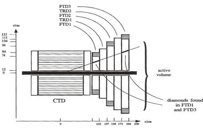
5.3 FTDFLT . . . 65
5.3.1 Introduction . . . 65
5.3.2 Diamonds . . . 66
5.3.3 Hardware . . . 69
6 The Regional First Level Trigger Box 72 6.1 Introduction . . . 72
6.1.1 Requirements . . . 72
6.1.2 Information Available to the RBOX . . . 72
6.1.3 Processing . . . 74
6.2 Simulation . . . 74
6.2.1 Geant and ZEUSGeant . . . 74
6.2.2 ZGANA . . . 77
6.2.3 Event Generation . . . 77
6.3 Details of the Algorithm . . . 81
6.3.1 Introduction . . . 81
6.3.2 Standalone FTD Subtrigger . . . 81
6.3.3 Standalone CTD Subtrigger . . . 81
6.3.4 Barrel Combined Subtrigger . . . 82
6.3.5 Forward Combined Subtrigger . . . 82
6.4 Results . . . 83
CONTENTS
6.4.2 Tracking Triggers . . . 89
6.4.3 Beamgas Background . . . 96
6.4.3.1 Comparison of Different Generators . . . 96
6.4.3.2 Reasons for Beamgas Leakage . . . 97
6.4.4 Calorimetry . . . 103
6.5 Hardware Design of the RBOX . . . 106
7 Investigation of Kinematic Dependence of CTDFLT Efficiency 109 7.1 Introduction . . . 109
7.1.1 Special Jacquet-Blondel Kinematics . . . 110
7.2 Event Generation . . . 110
7.3 Results . . . 112
7.4 Discussion . . . 115
7.5 Conclusions . . . 116
8 Heavy-Flavour Events in the Regional First Level Trigger 119 8.1 Introduction . . . 119
8.2 Simulation . . . 120
8.3 Results . . . 120
8.4 Discussion . . . 122
8.5 Conclusions . . . 123
9 Investigation of J/ΨEvent Acceptance in the FLT 129 9.1 Introduction . . . 129
9.2 Event Generation . . . 129
9.3 Results . . . 130
9.3.1 Trigger Efficiencies . . . 130
9.3.2 Comparison of Signal and Background . . . 130
9.4 Discussion . . . 133
9.5 Conclusions . . . 136
10 Conclusions 138
List of Figures
1.1 Feynman diagrams for electron-positron scattering in QED. . . 3
1.2 Feynman diagram for DIS. . . 13
1.3 The two lowest order QCD diagrams for BGF. . . 15
1.4 Lowest order diagram for inelastic J/Ψproduction. . . 16
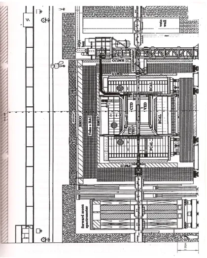
2.1 Section through the ZEUS detector along the beamline . . . 20
2.2 Arrangement of cells in the calorimeter. . . 22
2.3 The LPS stations along the straight section of the beamline. . . 27
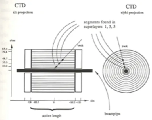
3.1 Central Tracking Detector Coordinate Systems. . . 31
3.2 Central Tracking Detector Coordinate Systems. . . 31
3.3 Sketch of an FTD subchamber. . . 35
4.1 Flow of data through the DAQ system. . . 38
4.2 Trigger regions in the calorimeter. . . 43
4.3 Forward muon detector first level trigger. . . 49
4.4 Barrel muon detector first level trigger. . . 49
4.5 LPS input to FLT: proton search. . . 50
4.6 Schematic of logic in the GFLTB. . . 52
5.1 Principle of the CTDFLT. . . 58
5.2 One of the 32 trigger sectors of the CTDFLT. . . 60
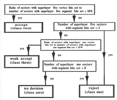
5.3 CTDFLT event classification flowchart. . . 63
5.4 Crossing misidentification. . . 65
5.5 Method of diamond forming. . . 67
5.6 Principle of the FTDFLT. . . 68
5.7 Outline of two-crate FTDFLT hardware design. . . 70
6.1 Mapping of the FTD onto CTD . . . 73
6.2 Typical values ofxfor physics sample. . . 79
LIST OF FIGURES
6.4 Subtrigger ratios for beamgas sample (zero bin removed). . . 84
6.5 Subtrigger ratios for CC sample (zero bin removed). . . 85
6.6 Subtrigger ratios for beamgas sample. . . 86
6.7 Subtrigger ratios for CC sample. . . 87
6.8 Profile of efficiency vs. leakage for CC events. . . 90
6.9 Profile of efficiency vs. leakage for NC events. . . 91
6.10 Cross-correlation plots for CC events. . . 92
6.11 Cross-correlation plots for NC events. . . 93
6.12 Beamgas leakage vertex profile along the beamline . . . 97
6.13 Number of track vertices per event. . . 100
6.14 Hit multiplicity distributions by event class. . . 101
6.15 Transverse and longitudinal momenta of tracks by event class for beam-gas. . . 102
6.16 Beamgas leakage vertex profile afterET cuts . . . 105
6.17 Regional box functional subdivision. . . 107
6.18 Regional box hardware scheme. . . 107
6.19 Subdivision in θof RBOX bitmap to GFLTB. . . 108
7.1 Contours of fixedyin thex−θjet plane. . . 111
7.2 Contours of fixedyin theQ2−θ jet plane. . . 112
7.3 Low statistics full angle pass for CC events. . . 116
7.4 Low statistics full angle pass for NC events. . . 117
7.5 Efficiency for CC events. . . 118
8.1 Effect of multiplicity and transverse energy on acceptance. . . 123
8.2 Multiplicity of charged tracks per event with apt>0.5GeV/c for heavy flavour events. . . 125
8.3 Total transverse energy (GeV) per event as measured by the calorimeter for heavy flavour events. . . 126
8.4 Total transverse energy (GeV) per event as measured by the calorimeter for beamgas events. . . 127
8.5 Multiplicity of charged tracks per event with a pt > 0.5 GeV/c for beamgas events. . . 127
LIST OF FIGURES
9.1 Sum of visible transverse energy in the electromagnetic calorimeter. . . 131
9.2 Sum of total transverse momentum (x-direction only). . . 132
9.3 Sum of total transverse visible energy. . . 132
9.4 Vetowall hits. . . 134
9.5 Number of hits in C5 collimator for J/Ψevents. . . 134
9.6 Number of hits in C5 collimator for beamgas events. . . 135
List of Tables
1.1 Quark doublets. . . 1
1.2 Lepton doublets. . . 2
2.1 Polar angle coverage of calorimeter sections. . . 23
2.2 Calorimeter readout tower size. . . 23
4.1 Rates of physics and background. . . 40
4.2 Processing time allowed per event by level of trigger. . . 40
4.3 Calorimeter tower numbers and makeup by location. . . 42
4.4 Total HAC and EMC energy deposited by a MIP by location of tower. . 44
4.5 FMUFLT polar angle subdivision. . . 47
5.1 Summary of CTDFLT event classifications. . . 64
6.1 Geant physics processes. . . 76
6.2 Kinematic variables of CC sample. . . 78
6.3 Proportion of beamgas events in zero bin with non-zero denominator for the four subtriggers. . . 88
6.4 RBOX FLT cut values for the four subtriggers. . . 91
6.5 Results for CC events. . . 94
6.6 Results for NC events. . . 95
6.7 Results for beamgas events. . . 96
6.8 Event classifications for different generators. . . 98
6.9 Transverse energy cuts chosen for the CTD. . . 103
6.10 Transverse energy cuts chosen for the RBOX. . . 103
7.1 CTDFLT efficiencies in the kinematic bins forθjet = 63◦±1◦. . . 113
7.2 CTDFLT efficiencies in the kinematic bins forθjet = 43◦±1◦. . . 113
7.3 CTDFLT efficiencies in the kinematic bins forθjet = 33◦±1◦. . . 114
7.4 CTDFLT efficiencies in the kinematic bins forθjet = 23◦±1◦. . . 114
LIST OF TABLES
7.6 Final combined figures for CTDFLT efficiency. . . 115
8.1 Percentage of events accepted by the simple parameterization of the tracking and calorimeter first level trigger. . . 121
8.2 FLT classifications for the full FLT simulations forc¯cevents. . . 121
8.3 FLT classifications for the full FLT simulations forb¯b events. . . 122
9.1 Event classifications from ZGANA. . . 133
Chapter 1
Physics at HERA
1.1 The Standard Model
Physics contains four fundamental forces: gravity, electromagnetism, strong and weak forces. The current understanding of particle physics is embodied in the ‘standard model’, which combines three of these forces in the framework of ‘gauge theories’
[1]. Quantum Electrodynamics (QED) describes forces between charged particles in
terms of photon exchange between them. This idea is extended to include the weak force (‘electroweak unification’), mediated by heavy W+,W−,Z0 bosons. Finally, in
quantum chromodynamics (QCD), gluons mediate the attraction which binds quarks in hadrons.
The model is in excellent agreement with experimental results, but contains more than twenty arbitrary parameters which must be adjusted to fit the data. It is hoped that as progress is made, this number will be reduced. Additionally, further steps towards a ‘grand unified theory’ containing all known forces are hoped for.
At the moment, the standard model envisages three families of quarks and leptons. The quarks are arranged in doublets.
Bound states of two or three quarks form mesons or baryons respectively. For example, two up quarks and a down form a proton. Leptons are currently thought to
doublet 1 doublet 2 doublet 3 charge
up charm top +2/3
down strange bottom -1/3
1.1 The Standard Model
doublet 1 doublet 2 doublet 3 properties
e µ τ large mass, charged
νe νµ ντ no mass or charge
Table 1.2: Lepton doublets.
be elementary and are also arranged in doublets as shown in table1.2. Here, heavy fermions are each accompanied by a neutrino.
1.1.1 QED
The Klein-Gordon (equation1.1) and Dirac (equation1.2) equations were devised as relativistic substitutes for the Schr¨odinger wave equation for fermions and bosons respectively
−∂
2φ
∂t2 = −∇
2 +m2
φ (1.1)
(iγµ∂µ−m) Ψ = 0 (1.2)
whereφandΨare the wavefunctions of their particles, m their mass, theγs are matrices constructed from Pauli spin matrices, and γµ∂
µ = γ0∂t∂ +γ · ∇. Quantum
mechanics postulates that wavefunctions may have arbitrary phase since phases do not influence any observable quantities. The requirements that the behaviour of particles under the equations is invariant under phase transformations constitutes the powerful ‘gauge principle’. In particular, there may be ‘local’ transformations: phase changes dependent on spacetime coordinates may be introduced. The gauge principle is equivalent to the demand that there should be invariance under the local transformation in equation 1.3.
1.1 The Standard Model
(a) (b)
Figure 1.1: Feynman diagrams for electron-positron scattering in QED.
However, the differential operators in both of the relativistic field equations equa-tion 1.1 and equation1.2 will now operate on the phase factorα so the invariance is lost. It transpires that it is necessary to introduce vector potentials in which the particles described move in order to offset the changes and restore the invariance.
In QED, these potentials may then be expanded in a perturbation series whose expansion parameter at each order is α, the fine structure constant. This is small:
α = 4πe2 = 1/137. The expansion allows the computation of amplitudes at a given order of α for scattering processes via consideration of four-vectors for incoming and outgoing particles and matrix elements representing the transition probabilities between initial and final states.
The amplitudes were represented in diagrammatic form by Feynman. A scattering process such ase+e− →e+e−was thus viewed at lowest order as onvolving exchange
1.1 The Standard Model
particle lines, and there are polarization vectors for any photons in the initial or final states.
Higher order correction terms in the expansion take the form of additional lines in the diagrams, For example, the diagram in figure1.1(b) allows for the possibility of virtual pair creation in the propagator. These corrections proved problematical: the relevant series diverge leading to unphysical infinite cross-sections.
The solution to this difficulty was found in the idea of renormalization. The inte-grals corresponding to loop corrections diverge at high momentum. Renormalization involves choosing an energy scaleΛQED above which no contribution to the amplitude
will be considered. This is equivalent to truncating the perturbation series after a fixed number of terms. It emerges that the infinities now cancel at each order: their effects are subsumed into the properties of the particle in question. it is not possible ever to measure ‘bare’ charge and mass because of these vacuum polarization effects.
Renormalized QED has shown remarkable predictive power. For example, the magnetic moment µof the electron is given by equation1.4
µ= ge 4me
(1.4)
whereg is the ‘gyromagnetic ratio’. The lowest order Dirac treatment predicts that
g = 2 exactly, but in the broader picture an electron must be regarded as an entity surrounded by virtual pairs. As discussed above, these alter its apparent properties and mean that summing corrections to higher orders produces a different prediction for g. This prediction and the measurement agree to ten significant figures.
1.1.2 Weak Interactions
1.1 The Standard Model
conserve charge and a neutrino to explain the observed energy spectrum. This picture has been modified (it is now based rather on quark transitions) but retains its validity.
In the framework of gauge theories, forces require a quantum to transmit their effects; intermediate vector bosons were postulated to fill this rˆole. These are now known to be charged W+ and W− together with the neutral Z0. These play an analogous part in the weak interaction to that of the photon in QED.
By the Heisenberg uncertainty principle, the range of a force is related to the inverse mass of its quanta. The masses (≥ 80 GeV/c2) of the Ws and Zs show that the range of the weak force is relatively small. Further, the propagator term in the cross-section formula depends onM−2W,Z, so the strength of the weak interaction is also comparatively small for low energy processes.
Weak interactions violate parity conservation: no process has so far been observed which involves a right-handed (i.e. positive helicity) neutrino. In the formalism, operators are formed fromγ5 which is a product of Diracγ matrices. The ‘V-A’ term
(1−γ5) projects out negative helicity states. Changing the sign of γ5 is equivalent to
introducing a ‘V+A’ component and would result in a projection of positive helicity states. This would then allow processes producing the unobserved right-handed neutrinos. Since these are not observed the framework describing charged current weak interactions is known as ‘V-A’ theory.
1.1.3 Electroweak unification
The unification of the electromagnetic and weak sectors is embodied in the theory of Glashow, Salam and Weinberg [2] [3] [4]. This requiredi) the devising of a mechanism
to generate mass for the weak bosons and ii) the identification of an appropriate gauge group.
Mass generation involves substitutions of derivatives analogous to equation1.5
1.1 The Standard Model
where
2 =∇2− ∂ 2
∂t2 (1.6)
so the interacting Maxwell equation for a massless photon
2Aµ=jµ (1.7)
becomes
(2+ M2)Wµ = 0 (1.8)
which is the equation for a free massive vector field. Considering only spatial components, this means it is necessary for the ‘screening current condition’ to hold:
i.e.that the current has a component proportional to the vector field.
j =−M2A (1.9)
This can only occur if an additional field is introduced. TheHiggs field[5] screens out the infinite range weak field which would result from having massless weak bosons.
It transpires that the correct gauge group here is SU(2)⊗U(1). SU(2) is the ‘weak isospin’ space in which there is a symmetry of the weak sector and U(1) represents the standard phase invariance of electromagnetism. The conserved quantity in the whole of this space is hyperchargeygiven by
1.1 The Standard Model
whereQis the electromagnetic charge andt3 is the third component of the weak
isospin quantum number.
There are two gauge fields in the resulting wave equation each of which have their own coupling strength. The linear combination of fields
g0Wˆ3µ+gBˆµ (1.11)
corresponds to the SU(2) and the U(1) parts of the overall gauge group. This represents a massless photon and a large mass W boson. The W mass is given by
MW = gf/2 (1.12)
where f is the vacuum expectation value of the Higgs field. The Z mass is related to this in terms of an angle which is the main free parameter of the theory
MZ=
MW
cosθW
(1.13)
This angle also fixes the relative strengths of the unified parts via
gsinθW =e (1.14)
1.2 Types of events at HERA
1.1.4 QCD
Considering baryons to be made up of three quarks had been shown to be productive prior to the advent of QCD. However, the Pauli exclusion principle was to force an extension to the simple quark model. The principle requires the wavefunction of a fermion to be antisymmetric; that is, under exchange of a pair of fermions, the wavefunction must change sign. Particles made up of an odd number of fermions are themselves fermions and thus the combined wavefunction of a baryon must change sign under exchange of one of its quark components. However, the ∆++ resonance
consists of three u quarks in identical spin states. It was therefore necessary to introduce an additional ‘internal’ degree of freedom to distinguish the quarks. This was termed ‘colour’. It is important to remember that free colour has never been observed, so all particles must be formed from colour neutral superpositions.
QCD is the theoretical framework which describes the strong interactions between quarks in terms of this colour charge. This is mediated by gluons which are themselves coloured and so can feel the influence of other gluons. This results in the phenomenon of ‘colour antiscreening’[?] in QCD. As the distance scale probed decreases, apparent
electric charge increases in QED. However, gluons reduce the effective coupling at smaller distances. This is why the ideas of perturbation theory, developed for weak forces, are applicable to QCD which describes the strong force. The theory is described as ‘asymptotically free’, meaning that as the distance scale probed grows smaller, so does the coupling. Conversely, this has the important consequence that quarks cannot exist in the free state: as two quarks are separated the bond strength between them increases to the point where pair production of new quarks takes place.
1.2 Types of events at HERA
1.2.1 Introduction
1.2 Types of events at HERA
been previously available[7]. This section will outline the processes relevant to the
work described later in this thesis. These fall into three main sections. Deep inelastic scattering events (DIS) are the mainstay of HERA physics. Secondly, many processes of interest take place via the mechanism of boson-gluon fusion (BGF). Finally more exotic processes are outlined.
The amount of data taken by an experiment is often quoted in units of inverse picobarns. A barn is 10−28m2. ZEUS is expected to accumulate 100pb−1
for each year of operation. This figure of ‘integrated luminosity’ may be multiplied by the cross-section for a given process to deduce the number of such events to be expected in a sample.
For example, the cross-section for top-quark pair production via photon-gluon fusion (see section 1.2.3.1) is dependent on the mass of the top quark. This now means that is unlikely to be much larger than0.01pband ZEUS is now thought to be unlikely to observe these events.
1.2.2 Deep Inelastic Scattering Events
1.2.2.1
Introduction1.2 Types of events at HERA
The topology of these events is generally described in terms of a particular formal-ism, described in the next section.
1.2.2.2
General KinematicsSeveral variables are used to describe event kinematics. Q2 is the squared
four-momentum transfer between the quark and the outgoing lepton.
Q2 =−q2 =−(pe−pl)2 (1.15)
the Bjorken variable
x= Q
2
2P ·q = Q2 2mpν
(1.16)
and the variable
y= P ·q P ·pe
= ν
νmax
(1.17)
In these equationspe,plandP are the four-momenta of the incoming and scattered
lepton, and the incoming proton respectively, andν = mq·p
p is the energy transferred by
the current in the proton rest frame.
In the limit of small lepton masses the variablesQ2,x andycan be determined
from the outgoing lepton energy Eland the lepton scattering angleθl(measured with
respect to the electron direction)
Q2 = 4EeElsin2
θl
1.2 Types of events at HERA
x= EeElsin
2θl 2
Ep Ee−Elcos2 θ2l
(1.19)
y= 1− El
Ee
cos2 θl
2 (1.20)
In CC events the neutrino energy and scattering angle cannot be measured by the detector but Q2,xandycan be calculated from the energy E
j and production angle
θj of the current jet (measured with respect to the proton direction)
Q2 = E
2 j sin2θj
1− Ej Ee cos
2 θj 2
(1.21)
x= Ejcos
2 θj 2
Ep
1− Ej Ee sin
2θj 2
(1.22)
y = Ej Ee
sin2 θj
2 (1.23)
Physically,xis the fraction of the proton momentum carried by the struck quark and can thus take values between 0and1. It is related toQ2 by a well known relation
which is shown in equation1.24.
Q2 =sxy (1.24)
1.2 Types of events at HERA
it is the fractional energy transfer in the laboratory frame and is given by dividing the energy of the exchanged boson by the incoming lepton energy. In a lepton-quark frame in whichsˆ=xsis the squared subprocess total energy,y= Qˆs2.
The value ofsat the HERA nominal beam energies is given by equation1.25.
s= 4EeEp = 98400 (1.25)
Clearly forQ2 to take this maximum value is it required thatx=y= 1meaning
thatallof the proton momentum is carried by the struck quark; y= 1corresponds to maximumQ2 for the particular struck quark.
1.2.2.3
Jacquet-Blondel KinematicsJacquet-Blondel kinematics consists of a parameterization of the above variables. The standard equations[8] expressQ2 in terms of jet angleθ
jet and energyEjet as follows:
Q2 = E
2
jetsin2θjet
1−y (1.26)
where
y= Ejet 2Ee
(1−cosθjet) (1.27)
This formalism is applicable to all CC and NC processes. At lowQ2 the scattering is
dominated by the pure electromagnetic term. AsQ2 increases, theγ/Z0 interference
term becomes important and finally above aroundQ2 = 104(GeV /c)2 the pure weak
term dominates.
1.2 Types of events at HERA
Figure 1.2: Feynman diagram for DIS.
from elastic1processes. The relevant Feynman diagram is shown in figure1.2.
1.2.2.4
Structure Functions and ScalingThe kinematical dependency of the DIS cross-section factorizes into leptonic and hadronic parts, each represented by a tensor.
dσ∼LµνWµν(q, p) (1.28)
whereq,pare four-vectors for the intermediate boson and the incoming hadron respectively. This leads to the following form for the NC cross-section
1If the scattering is elastic, then the four-momentum of the proton is unchanged by the collision:
1.2 Types of events at HERA
d2σ
N C(e±p)
dxdy = 4πα2
sx2y2
(1−y)F2(x, Q2) +xy2F1(x, Q2)±
y−y 2
2
F3(x, Q2)
(1.29)
in which three new parameters have been introduced. F1, F2 and F3 are the structure functions of the proton.
Bjorken scaling postulates that in the DIS regime, the Q2 dependence of the
structure functions should disappear, leaving only thexvariation. Intuitively, this is pictured as being related to the idea that at high Q2 the virtual boson interacts at
short distances inside the proton, essentially with only one parton. This may then be regarded as free on the short timescales involved and the scattering is elastic. Theny=xand the structure functions depend only on one variable. QCD predicts a violation of this scaling behaviour due to the addition of gluon loops.
1.2.3 Boson-gluon Fusion
1.2.3.1
Heavy-Flavour Pair ProductionThe phrase heavy-flavour conventionally refers to events involving the three heaviest quarks, that is the charm, bottom and the so far unobserved top quark. Events are mediated by the exchange of photons or bosons which fuse with a gluon radiated by the proton. This gives the BGF mechanism its name. The lowest order QCD diagrams are shown in figure 1.3.
The CC process is important for top production. However the total cross-section for all processes has a strong dependence on the quark mass[8]
1.2 Types of events at HERA
Figure 1.3: The two lowest order QCD diagrams for BGF. A quark/antiquark pair is formed.
At present, the top quark mass is thought to be 122+41−32GeV/c2 so it is no longer
expected that HERA experiments will be able to observe any top quark pair events. NC processes (in fact mostly gamma-gluon exchanges at lowQ2) dominate the BGF
cross-section.
1.2.3.2
J/ΨProductionJ/Ψ particles may also be produced by the BGF mechanisms shown in figure 1.4. Perturbative QCD has been used extensively to make calculations concerning c¯cpair production as a whole. This is a useful approach because the strong coupling constant
αS becomes relatively small at the charmed quark mass scale. This can be seen from
the leading logarithm approximation forαS as a running coupling constant1
αS(Q2) =
12π 21 ln(Q2/Λ2
QCD)
(1.31)
in whichΛis a QCD renormalization parameter.
1.2 Types of events at HERA
Figure 1.4: Lowest order diagram for inelastic J/Ψproduction.
The running of the coupling constant arises, analogously with the QED case, from choosing a mass scale at which to cut off higher-order diagrams with many loops. The running of the coupling constant is a consequence of the colour antiscreening mentioned previously. ClearlyQ2 can be regarded as a measure of the penetration of
the probe so it is expected that the coupling will decrease with higher Q2.
ΛQCDhas been found to be between0.1→0.2GeV. The cross-section is dominated
by almost real photons: Q2photon = 0 so the gluon must have Q2
gluon ' MΨ2. From
equation 1.31it can be seen that the coupling is relatively weak at the relevant mass scale.
Data so far available (e.g. EMC) supports the ‘colour singlet’ model of Berger and Jones[9]as the mechanism for J/Ψproduction. The model successfully reproduces the
transverse momentum and Q2 dependence of the EMC data[10].
In order to extrapolate cross-sections down to the very low Q2 domain of J/Ψ
production, the Weizsaecker-Williams approximation[11] is important. it states that the
1.2 Types of events at HERA
other is dependent on the emitted photon and initial particle energies.
The J/Ψ cross-section is sharply peaked in x just above x ' m2Ψ
s
[12]. Because
HERA is a high energy machine with large and variable s, the peaks occur at much lower values of x than at previous experiments so these events will be useful to probe the gluon distribution[13] in a new domain. They will have extremely lowQ2
(10−4GeV2 ≤Q2 ≤10−2GeV2 for example) and hence a very small scattered electron angle.
1.2.4 Exotica
Three main avenues for investigation of exotic physics[14] exist at HERA. These are
searched for excited electrons, leptoquarks/leptogluons and supersymmetry. The crucial parameter in this context at HERA is √s = 314GeV, which is the amount of energy available in the centre of mass frame for the creation of new states.
1.2.4.1
Excited ElectronsThe existence of excitations would indicate that the presence of a previously un-detected substructure. This would require another internal degree of freedom like colour: all observed states would be ‘hypercolour’ neutral. Hypergluon exchange would confine preons on some compositeness scale. The excited states decay (e.g.
l∗ →e+γ or q∗ →q+W±) so construction of invariant mass plots from the decay products should prove a useful method of investigation.
1.2.4.2
Leptoquarks and LeptogluonsThese are resonant states between leptons and partons[15]. Leptoquark production
occurs at fixed x(x=mleptoquark/s). The events are similar to DIS, which forms the
major background. The DIS cross-sections show aQ−4dependency whereas leptoquark decays are isotropic: they will show no Q2 dependence. Thus selecting events with
1.2 Types of events at HERA
1.2.4.3
SupersymmetrySupersymmetry, or SUSY, envisages a more broad symmetry than the usual multiplet schemes. Here, fermions and bosons may be members of the same gauge group multiplet. A usual, however, the supersymmetry must be broken in a manner consistent with low-energy phenomenology.
The minimal model gives each particle a SUSY partner so that there are now eight gluinos as well as the familiar gluons and also there are squarks and sleptons. Processes analogous to standard DIS are envisaged in which the gauge boson is replaced by a gaugino (e.g. a Zino or a Wino). This leads to a squark and a selectron in the final state.
The cross-sections for production at HERA should be sufficient to observe SUSY-NC processes providing that
Chapter 2
Non-Tracking Elements of the ZEUS
Detector
2.1 Introduction
The ZEUS detector consists of three main types of detector: those which are sensitive to charged tracks, those that measure energy deposition and those which identify muons. The UK’s major responsibility on ZEUS is the Central tracking Detector (CTD). Because of this and the fact that a large part of the work outlined in this thesis has been connected with tracking components, their description deserves a separate chapter, which follows.
The tracking detectors reside in the inner region close to the interaction point. The remaining major components fall into two functional classes: calorimetry and muon detection.
2.1 Introduction
2.2 Calorimetry
2.2 Calorimetry
2.2.1 Introduction
The purpose of the calorimeter is to investigate jet properties by measuring their energy deposition. The design aims to cover the full solid angle so far as is consistent with the presence of the beamhole. It allows for the discrimination of jet angles with resolution of better than 10 mrad. Discrimination between hadrons and electrons is foreseen. The resolution on the jet energy should be
σ(Ejet)
Ejet
= p 35%
Ejet(GeV)
⊕2% (2.1)
The calorimeter at ZEUS has been designed to be ‘compensating’i.e. it will give the same response per unit energy irrespective of whether the depositing particle is electromagnetic or hadronic. This reduces the systematic error in the energy measurement, as can be seen from the following example. In a given event π0 day leads predominantly to electromagnetic showers visπ0 →2γ whereas chargedπs will
give a hadronic deposition. So in an uncompensated calorimeter the measurement of a set of events with the same energy would depend on the ratio of charged to unchargedπs in the events.
ZEUS has adopted a compensating calorimeter of depleted uranium/scinitillator design. Here the high-Z absorber plates are interleaved with plastic scintillator tiles which are read out by photomultiplier tubes. Achievement of compensation requires careful consideration of the layer thicknesses because of the different cross-sections for the various processes via which hadronic and electromagnetic particles lose energy.
2.2 Calorimetry
Figure 2.2: Arrangement of cells in the calorimeter.
encountered by particles emanating from the interaction region. There are two layers of HACs behind these in the FCAL and the BCAL and one layer in the RCAL.
2.2.2 Forward, Rear, Barrel Calorimeter (F/R/BCAL)
The calorimeter has three major sections. Their coverage in terms of polar angle and depth is shown in table2.1. Depth is measured in radiation lengths ,X0, over which
distance the energy of an electron will be reduced by a factor ofe. it can be seen that there is some angular overlap between sections.
Each section has one interaction length of EMC at its face closest to the interaction point. Behind that, the layer of HACs varies from '6λ in the forward direction to
2.2 Calorimetry
Region Coverage X0(EMC) X0(HAC) λ(total)
FCAL 2.2◦ →39.9◦ 26 162 5.6→7.1
BCAL 36.7◦ →129.1◦ 25 103 5.3
RCAL 128.1◦ →176.5◦ 26 81 3.3→4.0
Table 2.1: Polar angle coverage of calorimeter sections.
Tower location Dimension
FEMC 5×20cm2
REMC 10×20cm2
BEMC 5×24cm2
HAC 20×20cm2
Table 2.2: Calorimeter readout tower size.
2.2.3 Backing Calorimeter (BAC)
The BAC, together with the iron return yoke, is between the inner and outer muon chambers. It is designed to be complementary to the main calorimeter and the muon chambers. It will allow measurement of late-showering particles and it will provide a muon trigger in the bottom yoke where there will be no muon chambers.
There will be around 9 layers of BAC modules depending on the exact location. The layers are made up of either 7 or 8 tubes which each contain one gold/tungsten wire and use an argon/CO2 gas mixture. Four modules will be grouped on readout into
towers of around50cm×50cmbase and summed in depth. The final position resolution should be 1.3mm and the design energy resolution for hadrons is σ(E)E '100%/√E.
2.2.4 Hadron Electron Separator
2.3 Muon Detectors
resolution.
The diodes are operated in depleted mode. The passage of a charged particle creates many charge carriers. The resulting pulse is readout and is of different heights for electrons and hadrons even if they are of the same energy. The ability of the calorimeter as a whole to distinguish electrons is therefore improved. Using only HES data, electron identification efficiency of90%should be obtainable with only 4%
hadronic contamination.
2.3 Muon Detectors
2.3.1 The Forward Muon Detector (FMUON)
This component is based on a toroidal magnet. Its detectors comprise streamer tubes and drift chambers, both of which measure ionization, and a time-of-flight (TOF) plane between the two toroids. It comprises in addition to two ‘wall’ sections (LW1,2) a ‘spectrometer’ section with five detector planes. These five planes are labelled LT1
→LT5. Particles from the interaction region encounter the wall sections first and then the spectrometer. The walls provide overlap of angular coverage with the BMUON. The planar sections are divided into eight sectors in φ. The TOF plane consists of sixteen elements, each are made up of a pair of scintillation counters separated by 10cm.
This component will provide small angle muon momentum resolution of20%. This information is essential to complement tracking detector data. The purpose of the TOF plane is to ensure that particles are not associated with an incorrect beam crossing.
2.3.2 Barrel/Rear Muon Detectors (B/RMUO)
2.4 Other Elements
barrel and are placed horizontally in the RMUO. These are readout by time-to-digital converters. Analogue readout of strips in the orthogonal dimension is available in both cases.
2.4 Other Elements
2.4.1 The Vetowall (VETO
This is a large iron wall seven metres in front of the interaction region which has a hole in it through which the proton beam passes, It has hodoscopes on each side consisting of forty-eight individual scintillation counters.
There is a ‘halo’ of protons not following the nominal beam trajectory and these may produce highly penetrative muons by collision with machine elements. The main purpose of the vetowall is to veto these events and thus reduce the rate of spurious triggers in the detector.
2.4.2 The Luminosity Monitor
The measurement of cross-sections is of primary importance at ZEUS. This requires monitoring to arrive at the figure for time integrated luminosity. It is essential also to have the information online so as to be able to optimize the luminosity in the interaction region.
In order to do this, the LUMI uses the process of photon emission from the interaction of the two beams ep→epγ. Also, the LUMI will identify photoproduction processes by tagging small-angle electrons.
The detector itself has two parts, an electron detector near the electron beam at z=-36m and a photon (γ) detector around the proton beam at z=-108m. The electron detector is a shielded lead/scintillator sandwich. Theγ-detector is based on a
γ-calorimeter which consists of layers of 1cm2 silicon pads. A photon causes a shower
2.4 Other Elements
counter to veto electrons is included in the design; a prototype has been built using a
150cm thickness of polyurethane foam.
2.4.3 Leading Proton Spectrometer (LPS)
It is expected[16] that in 25% of DIS events, the proton will interact diffractively,
retaining its identity and losing momentum. If this happens, it may then leave the beampipe and be measured by the LPS with efficiency'0.6at the most favourable momentum.
The LPS will have six detector stations along the proton line between z=+24m and z=+90m as shown in figure2.3. These will be based on turret extensions into which ‘pots’ can be inserted. pots contain detector elements: their purpose is to allow for precise control of location of the detectors over the last few centimetres close to the beampipe.
The first three stations will have a single pot and the last three will be double pot assemblies. The single pots will be horizontal with respect to the beamline and the double pots will be vertical. The exact location of the detectors is important because it determines the proton phase space acceptance of the LPS.
Each pot will contain a detector element comprising seven planes of silicon mi-crostrips with differing orientations to provide two-dimensional measurement and will be shaped to fir closely to the beampipe. The total area covered by the strips will be 1560 cm2
2.4.4 Rucksack
2.4 Other Elements
2.4 Other Elements
The rucksack is connected to the components via a dragchain which is designed to carry cables for readout. The rucksack must be mobile. This is because the yoke -the large iron clamshells and -the BMUO/BAC - retracts to allow access to -the inner detectors. The rucksack moves in the same rails in which the yoke runs.
2.4.5 Solenoid
A magnetic field must be supplied in the region of the tracking detectors so that charged tracks will bend in it and thus their momentum may be measured. A1.9 m
Chapter 3
Tracking Elements of the ZEUS
Detector
3.1 Introduction
Both of the experiments planned for HERA, ZEUS and H1, have specialized tracking detectors in the forward direction because of the beam asymmetry mentioned pre-viously. At ZEUS, there are four separate tracking chambers. The system as a while can take measurements of varying degrees of accuracy for tracks with polar angles between7.5◦ and170◦.
All of the tracking detectors are wire drift chambers in which the passage of a charged particle leaves a trail of ionization. Anode wires in each chamber are equipped with electronics to readout pulses due to the arrival of charge produced by this ionization.
All of the chambers are designed to operate in a high magnetic field. This causes particle trajectories to bend thus enabling momentum measurement. The tracking detectors differ in their geometry and in gas mixture, field shape and strength depend-ing on their location. In particular, the magnetic field is highly non-uniform in some regions and this has had to be taken into account.
3.2 The Central Tracking Detector (CTD)
3.2 The Central Tracking Detector (CTD)
3.2.1 Introduction
The CTD has an overall length of 240 cm with inner radius of 16.2 cm and outer radius of 85 cm. However some space must be left inside the chamber to house readout electronics, and allow for cabling and cooling requirements. The sense wires are strung along the205 cmactive length of the chamber between two 20 mmthick aluminum endplates.
The requirements which the CTD was designed to satisfy are:
• Event triggering by vertex measurement (i.e.rejection of upstream gas), see section5.2.
• High resolution momentum measurement of tracks.
• Identification of electrons by measurement of energy loss.
3.2.2 Mechanical Construction
The CTD[17]is radially subdivided into superlayers (SLs) which are numbered from
one at the smallest radius to nine at the largest. Each SL thus forms an annular cylinder eight wires thick. There are two types of SL. In the axial SLs, the sense wires run parallel to the z-axis (see figure 3.1). In the stereo layers however a twist of five degrees has been introduced corresponding to a two-sell displacement at the endplates, in order to allow reconstruction of the z-coordinate of the tracks.
3.2 The Central Tracking Detector (CTD)
Figure 3.1: Central Tracking Detector Coordinate Systems.
3.2 The Central Tracking Detector (CTD)
Cells consist of the eight sense wires plus a variety of other wires which are all designed to supply and shape the electric field within a cell such that electron drift trajectories are uniform. The maximum drift distance is 25.6 mm.
The uniform electrical field within each cell means that the drift velocity is inde-pendent of trajectory within the cell, simplifying reconstruction. It would be helpful if the drift velocity could be fixed such that the maximum drift time was small compared ti the beam-crossing interval. This would minimize difficulties in identifying which crossing a particular track is associated with. this would indicate a small cell size, but this would then require a larger number of wires to be readout. SO the cell size has been fixed at'2.5 cmwhich maintains a small probability that two events will overlap in the same cell, satisfies the requirement that a not unreasonably large number of wires must be readout, and produces a maximum drift time of500 ns.
3.2.3 Electronic Readout
There are a total of4608sense wires in the CTD. It is necessary to terminate the wires in the390Ωcharacteristic impedance of the chamber in order to prevent pulses being reflected back into it. At the FTD end, this is done by a resistor network (for those wires not equipped with z-by-timing readout). At the RTD end, it is done by preamp. cards[18] which are designed to increase the signal strength.
The preamps are connected to42 m long high quality coaxial cables which run through the dragchain. This connects the chamber to the rucksack (section 2.4.4) which houses the majority of the electronics. Postamp boards amplify the signals. At this point the readout chain splits into two with both parts simultaneously being fed data. Both parts are concerned with coordinate identification in different planes.
3.2.3.1
R-φ CoordinatesThe pulses from the postamps are sampled by 8 bit 104 MHz flash analogue-to-digital converters (FADCs). The results are continuously written to 512 location deep pipelines. Onboard Digital Signal Processors (DSPs)[19]1 produce drift times and do
1DSPs are microcomputers providing several MIPS of computing power and suited to high data
3.2 The Central Tracking Detector (CTD)
pulse height/area analysis.
The radius of a hit is defined by the wire number, Theφcoordinate may then be found from this and the drift time. There is, however, a left-right ambiguity. The drift time may be used to find the distance from the sense wire plane of the ionization causing it but not on which side of the wire it was produced. This has the effect that two sets of hits are found in each cell. Because of the 45◦ angle of the sense wire planes, one of these sets does not point to the interaction region and can be easily discarded. The design resolution is100µm.
3.2.3.2
Z-coordinateThere are two methods of measuring the remaining z-coordinate, with differing degrees of precision. All of the sense wires in SL1 and half of those in SL3 and SL5 are instrumented for z-by-timing[20]. Those wires which are instrumented have preamps
at both ends of the chamber and corresponding postamps in the rucksack.
On a given wire, pulses arrive at different times at the two ends of the chamber depending on where along the wire the ionization was produced. Preamplifiers mounted on the chamber drive the signal along coaxial cable to the rucksack where postamplifiers feed into constant fraction discriminator units. One end of the chamber has an extra 10 nsdelay so that the pulses will always arrive in the same order. This enables time-to-amplitude conversion to take place based on charging a capacitor starting from the arrival of the start pulse and ending with the arrival of the stop pulse. The time difference is then proportional to the charge on the capacitor which is sampled by a FADC which has seven bits available to measure the z-coordinate. The design resolution is 3 cm[21]. The FADC data is sent to the pipeline (section 4.3.1), which is read out in the event of a trigger.
3.3 Forward Detector (FDET)
of the z-coordinate. At present it is likely that this data will only be used in the full event reconstruction, where it should provide a resolution in z of1.2 mm.
3.3 Forward Detector (FDET)
The FDET consists of three FTD subchambers with two TRD modules in the gaps between them.
3.3.1 The Forward Tracking Detector (FTD)
A drawing of a subchamber is shown in figure3.3. The FTD is intended to complement the angular coverage of the CTD and is crucial in providing data relating to tracks close to the beampipe.
Each of the FTD subchambers contains three readout planes, each containing more than a thousand wires. The sense wires are parallel to each other within a plane but there is a 60◦ offset between the planes to permit three dimensional hit location. The Siegen group is designing100 MHzFADC cards similar to those that have been produced for the CTD which will be used to readout the FTD. However, the design here will be simpler.
3.3.2 The Transition Radiation Detector (TRD)
Charged particles crossing an interface between materials having different dielectric properties will lose energy by emission of photons. These photons will in turn transfer energies to atomic electrons via excitation and ionization processes. In this way, if the original particle was sufficiently energetic, an electromagnetic shower may be built up.
3.3 Forward Detector (FDET)
3.4 The Rear Tracking Detector (RTD)
interactions. The shower results in an anode pulse which is read out by FADCs as in the CTD. The primary purpose of the TRD is to permit electron tagging. Transition
radiation is not produced byπs with momentum below40 GeV/c[22] so whileπs and electron have similar dE/dx characteristics the pulse shapes produced will differ. This should allow the TRD to distinguish between the two with a discrimination factor of 100 (for electrons with energies between1 GeVand30 GeV).
3.4 The Rear Tracking Detector (RTD)
The RTD is basically identical to one FTD subchamber but of slightly smaller size. Its sensitive volume extends down to 10◦ in the rear direction.
3.5 The Vertex Detector (VXD)
In order to obtain improved resolution, the design of the VXD progressed assuming the use of a ‘slow’ gas; dimethyl ether was chosen. This then meant that the cell size would be smaller than in the CTD in order to restrict drift times to a reasonable length. Constraining the number of readout channels led to a maximum drift time of
500 nsover a distance of no more than3.6 mm. There are twelve sense wires at3 mm
intervals in a VXD cell.
Chapter 4
The ZEUS Trigger Environment
4.1 Introduction
Triggering is the selection of physics events of interest in conjunction with the rejection of background processes which it is not desired to investigate. The success of any HEP experiment is critically dependent in its ability to achieve a high trigger efficiency. Identification of interesting physics must be as close to perfect as possible in order to avoid the introduction of unacceptable systematic errors and to maximize the amount of recorded data relating to physics events. A trigger is a complex entity comprising, at HERA, readout electronics, hardwired algorithms and much sophisticated software running on powerful dedicated processors well matched to particular tasks.
At HERA, triggering has assumed even greater importance than in the past partly due to the high rates of background and partly due to the short beam-crossing interval of only96 ns. At other machines, a longer interval simplifies trigger design so that no pipelining of data is required. For example, the Large Electron-Positron collider at CERN has a crossing every10µs. Experience gained at HERA will prove invaluable in the design of the yet more complex triggers which will be required at the next generation of colliders, notably the Superconducting Supercollider in Texas which will have a beam crossing interval of16 ns.
4.1.1 Overview of Dataflow
4.2 Rates and Background
Figure 4.1: Flow of data through the DAQ system.
acquired for the event and sends it to the third level trigger (TLT). This, mediated by the Central Data Acquisition (CDAQ) VAX and run control (RC), writes events passing the final stage to tape. There is also some facility for local disk storage.
4.2 Rates and Background
4.2 Rates and Background
It is envisaged that there will be three main sources if background in ZEUS; cosmic rays passing through the detector, losses from the proton beam, and interactions of the beam with residual gas inside the beampipe. The latter are known as beamgas
interactions and much effort has been expended to try and devise triggering strategies to prevent them from causing triggers.
Cosmic ray events will on the whole be rejected by the use of timing information from the calorimeters.
Protons not following the nominal beam trajectory hit machine elements thus producing hadronic showers including pions. These can subsequently decay into muons which are very penetrating. There are approximately2×1013 protons in the
beam. The circumference of the ring is 6336 m If it is assumed that the beam will have a lifetime of about ten hours, these interactions may occur at a rate of up to
100 kHz per metre of beamline. However, structural elements such as collimators, beam scrapers and the vetowall will substantially reduce the rate of these events causing activity in the detector.
It is estimated that the rate of beamgas interactions will be up to2kHzper metre[23].
Near the interaction region they will fake good events in the tracking trigger. Upstream of it, their modest energy deposition may be misinterpreted by the calorimeter as a high transverse energy deposition representing a large Q2 interaction. This is because upstream tracks which are in fact only leaving the beampipe by a shallow angle can arrive a long way away from it once they are intercepted at the interaction region. Also, upstream beamgas can have secondary interactions producing tracks which come from the interaction region. This background is potentially the most serious.
4.3 The Trigger
Assuming the design luminosity of1.5×1031cm2s−1 leads to the rates shown in table4.1for events observed in the acceptance of the ZEUS detector.
Process Rate
DIS NC 0.075 Hz
DIS CC 0.001 Hz
BGF J/Ψ 0.045 Hz BGFb¯b 0.015 Hz
beamgas 100kHz
cosmic rays 5kHz proton halo ∼100kHz
Table 4.1: Rates of physics and background.
4.3 The Trigger
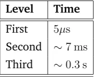
As mentioned above, the ZEUS trigger will have three levels. In order to allow more sophisticated processing on a more complete subset of component data at successive levels, each level will have a longer period of time with which to make a decision. This is shown in table4.2.
Level Time
First 5µs
Second ∼7 ms
Third ∼0.3 s
4.3 The Trigger
4.3.1 The First Level Trigger
it is impossible to decide whether or not to accept an event within the96 nsbetween beam crossings. In the first level trigger (FLT)[24] [25] [26], this forces the storage of
data in pipelineswhich must be able to hold data relating to 5µs.
Processing takes place both at the level of individual components and in theGlobal First Level Trigger Boxor GFLTB[27] [28] [29] [30] [31] [32]. because of these constraints the
sophistication of processing that may be done by components at this level is restricted. The output rate from the FLT will be1 kHz, after the fast clear section4.3.1.2.
The components must write the data relating to the event to their internal pipeline. Each of the components have26beam crossings to perform calculations on their data. They must then send the results of these calculations to the GFLTB. If the GFLTB decides to accept the event, it will send an accept bit to each component exactly20
beam crossings later. The GFLTB must therefore complete its calculations within this 20 beam crossing period. The components then read out the relevant data to the
component second level trigger.
The tracking detector FLT is is central to the work presented in this thesis. Its discussion is therefore postponed to the following chapter.
4.3.1.1
Calorimeter FLTThe calorimeter first level trigger (CALFLT) [32] [33] [34] is designed to detect isolated
4.3 The Trigger
deposition in order to recognize patterns associated with good events.
The original intention to measure longitudinal momentum will not now be fulfilled due to financial reasons.
The calorimeter is mostly non-projective: only the electromagnetic section of the barrel has cells aligned parallel to lines radiating from the interaction point. For this reason, the subdivision of the calorimeter into regions for trigger purposes is different to its physical division. Entities known as ‘trigger towers’ are formed from calorimeter cells such that a straight line from the interaction point will be fully contained within them.
Most towers contain two electromagnetic calorimeter (EMC) cells representing approximately 25 radiation lengths as was shown in table2.1. Beyond that are the two paris of HACs (hadronic cells) which map most closely on to the EMCs. In a small number of towers at the edges of the FCAL and of the RCAL, the BCAL is between the first cell in the tower and the interactions region. In this case, the tower contains only HACs (see section 2.2.1). The makeup and number of towers in the calorimeter is shown in table4.3.
Region Number of towers Number with EMCs
FCAL 460 264
BCAL 448 448
RCAL 452 262
sum 1360 974
Table 4.3: Calorimeter tower numbers and makeup by location.
4.3 The Trigger
Figure 4.2: Trigger regions in the calorimeter.
division emerge from this process. The calorimeter is now divided into sixteen trigger regions: four for each of the RCAL and FCAL and eight for the barrel. This is shown in figure4.2. Each region contains7×8towers.
Each calorimeter cell is read out by two photomultiplier tubes. EMC and HAC energy depositions are summed within a tower by onboard cards known as trigger sum cards (TSCs). These sums are sent to trigger encoder cards (TECs) in the rucksack: each TEC covers four towers. So there are14TECs in a crate to cover the56towers in each of the sixteen trigger regions.
For each tower, EMC and HAC energy deposition is measured on two digitization scales by flash analogue-to-digital converters (FADC): high gain (12.5 GeV on an 8
bit scale) and low gain (400 GeV over 8 bits in the FCAL and 100 GeV over 8 bits in the RCAL and BCAL). If the deposition exceeds a scale an overflow bit is set. If neither the HAC nor the EMC in a tower set off the high-gain channel, the TEC ceases to perform energy sum calculations and begins testing for electrons and minimum ionizing particles as described later.
4.3 The Trigger
uses these and the finest resolution energy scale available (depending on whether the high or low gain channel has been used) to find transverse energy depositions. Total and transverse energy sums for the four towers covered by each TEC are sent to a trigger adder card (TAC). There are two of these in a crate.
The TEC’s run test procedures may result in three bits being set for each tower. An E-bit is set if the depositions found are characteristic of an isolated electron: these will predominantly deposit their energy in the EMC part of a tower. The design aims to find all electrons with energy greater than5 GeV.
The EMC threshold is set at 2.5 GeV however since an electron may deposit its energy in adjacent cells. Since there is a small likelihood that an electron with energy between 2.5 GeVand5.0 GeVwill ‘punch through’ the EMCs to reach the HAC layer, only 0.1 GeV is allowed in the HAC layer. If the EMC deposition is greater than
5.0 GeV, then the ratio EEMC
EHAC must be greater than10. A slightly different requirement
is implemented in the more active FCAL but clearly the requirement for this bit to be set is also based on substantial symmetry between the two types of cell.
The rate at which charged particles passing through matter lose energy by ion-ization depends on their energy. In fact, the rate decreases to a minimum and then increases to a plateau at high energy. Particles above the minimum are called mini-mum ionizing particles or MIPs. The energy deposited by a particle at the minimini-mum in a tower is shown in table 4.4.
Cell Type EMIP/MeV
BEMC 321
BHAC 1360
FEMC 363
FHAC 2268
Table 4.4: Total HAC and EMC energy deposited by a MIP by location of tower.
4.3 The Trigger
deposition E fulfills the condition 0.2EMIP ≤ E≤2EMIP. It is generally likely that a
muon is the cause. Muons are comparatively penetrating and so do not deposit most of their energy in the EMCs. Genuine hadrons will usually have energies which are much too large to set the M-bit.
Towers in the active region around the beampipe are not permitted to set E or M bits. If insufficient energy is deposited to set either of these bits, LUTs are used to find if the tower is ‘low-activity’ for the Q-bit. ‘Q’ stands for ‘quiet’. In fact, the requirement to set the Q-bit is that the pulse height be less than 20%of the pulse height required to set the M-bit.
In the TACs, pattern logic searches for groups of up to four E or M-bits set and surrounded by Q-bits in each of the sixteen regions. NC events have a high-energy isolated electron and this pattern logic forms an excellent trigger on these events. On the other hand, isolated muons are characteristic of many interesting physics processes including heavy quark production.
The exact thresholds for these bits vary depending on the location of the tower being processed. The thresholds for the E, Q and M-bits must be matched to each other because otherwise a legitimate electron may fail its isolation requirement. Therefore a quiet tower is defined by having less than the minimum EMC energy for an E-bit and the minimum HAC energy for an M-bit. For example in the FCAL a quiet tower must haveEEMC <2.5 GeVandEHAC<2.268 GeV. These bits are sent to the CALFIT
processor.
The CALFIT processor receives the energy sums for the sixteen regions and also on a finersubregionscale. This finer scale is designed to have better resolution around the beampipe and to prevent loss of the flexibility to examine data relating to areas covered by more than one trigger crate. The CALFIT processor will be able to examine in this way deposition in the FCAL and the RCAL in annular regions at different radii from the beampipe. this is useful because beamgas events are more likely to have high deposition around the beampipe region than physics events for Q2 values of interest
4.3 The Trigger
Sums are made of the number of towers in each region which have energy sufficient to set the bits. This enables the processor to search for jets which will appear as clusters of towers with bits set.
The processor sends data to the GFLTB relating to the whole calorimeter and to the
16subregions. The global data is: EEMC,EEMC+ EHAC,ExEMC+ ExHAC,E y
EMC+ E y HAC ,
Ex EMC ,E
y
EMC , missing energy, cluster data and the total number of E and M-bits set.
Further, the result of a beamgas likelihood algorithm1 is sent. On the subregion scale,
the M and Q-bitmaps are sent to the GFLTB long withEtot ,Etrans ,Eemc,Ex andEy.
4.3.1.2
Fast ClearTo ensure that the accept rate to the second level trigger is no greater than1 kHzan element of parallel processing of calorimeter data has been introduced[35]. The fast
clear (FC) will consider data simultaneously from the FCAL, RCAL and BCAL relating to events which have had an FLT issued. Each accept is accompanied by an indication of whether the GFLTB will permit the FC to abort the event, based on the strength of its acceptance by components other than the calorimeter.
The FC works by searching for clusters[36] and finding their angle and energy. Cuts
are made to discriminate against beamgas which can be quite stringent compared to those in the FLT because the FC will be permitted to abort a trigger only if the other components show a weak accept decision.
An important quantity in the FC is shown in equation4.1
Ef =
EEMC(RCAL)−EHAC(RCAL)
EEMC(RCAL) + EHAC(RCAL)
(4.1)
In CC events, hadron jet do not often have trajectories which take them through the RCAL. On the other hand, about 80% of particles in beamgas interactions are hadronic. So physics events have high-angle clusters with largeEf. It has been shown
that a cut based on this ratio for the highest energy cluster in the RCAL yields a
1This uses the regional energy sums and also the sum of energy in the beampipe region (because