Scand J Med Sci Sports. 2018;28:2263–2271. wileyonlinelibrary.com/journal/sms
|
22631
|
INTRODUCTION
Near- infrared spectroscopy (NIRS) is a common tool to indirectly measure muscular oxygen availability and mi-crovascular reactivity noninvasively.1-5 Implementation of NIRS relies on the transparency of human tissue and the light absorbing characteristics of oxy- (O2Hb) and deoxyhaemoglobin (HHb) chromophores for the determina-tion of their concentradetermina-tion ([O2Hb] and [HHb], respectively) in a localized tissue bed.6 Changes in [O
2Hb] and [HHb]
reflect the dynamic balance between muscle oxygen (O2) delivery and extraction in the underlying tissue.7 In contin-uous exercise where NIRS responses are relatively stable, averages can be calculated over discrete and predetermined time points for identification of overall trends within the exercise bout.1,2 When maximal sprint efforts are repeated, however, there is a rapid deoxygenation at exercise onset that slowly recovers at sprint cessation.8-10 The evolution of peaks and nadirs across the NIRS signal is often used to describe the quality of metabolic recovery between sprint O R I G I N A L A R T I C L E
Influence of averaging method on muscle deoxygenation
interpretation during repeated- sprint exercise
R. F. Rodriguez
1|
N. E. Townsend
2|
R. J. Aughey
1|
F. Billaut
1,31Institute for Health and Sport, Victoria
University, Melbourne, Australia
2Aspetar, Doha, Qatar
3Department of kinesiology, University
Laval, Quebec, Canada
Correspondence
François Billaut, Department of
kinesiology, Faculty of medicine, University Laval, Quebec, Canada.
Email: [email protected]
Near- infrared spectroscopy (NIRS) is a common tool used to study oxygen availability and utilization during repeated- sprint exercise. However, there are inconsistent methods of smoothing and determining peaks and nadirs from the NIRS signal, which make inter-pretation and comparisons between studies difficult. To examine the effects of averaging method on deoxyhaemoglobin concentration ([HHb]) trends, nine males performed ten 10- s sprints, with 30 seconds of recovery, and six analysis methods were used for deter-mining peaks and nadirs in the [HHb] signal. First, means were calculated over predeter-mined windows in the last 5 and 2 seconds of each sprint and recovery period. Second, moving 5- seconds and 2- seconds averages were also applied, and peaks/nadirs were de-termined for each 40- seconds sprint/recovery cycle. Third, a Butterworth filter was used to smooth the signal, and the resulting signal output was used to determine peaks and nadirs from predetermined time points and a rolling approach. Correlation and residual analysis showed that the Butterworth filter attenuated the “noise” in the signal, while maintaining the integrity of the raw data (r = .9892; mean standardized residual −9.71 × 10³ ± 3.80). Means derived from predetermined windows, irrespective of length and data smoothing, underestimated the magnitude of peak and nadir [HHb] com-pared to a rolling mean approach. Consequently, sprint- induced metabolic changes (in-ferred from Δ[HHb]) were underestimated. Based on these results, we suggest using a digital filter to smooth NIRS data, rather than an arithmetic mean, and a rolling approach to determine peaks and nadirs for accurate interpretation of muscle oxygenation trends.
K E Y W O R D S
Butterworth filter, deoxyhaemoglobin, near-infrared spectroscopy, tissue oxygenation
© 2018 The Authors Scandinavian Journal of Medicine & Science In Sports Published by John Wiley & Sons Ltd
bouts.9,11,12 Because of the rapid oxygenation adjustments and short duty cycle of repeated- sprint exercise,10,12,13 ac-curate identification of peaks and nadirs in the NIRS signal is critical.
Analysis of NIRS data obtained during repeated- sprint ex-ercise is often constrained to [HHb]8,11,13-15 due to Δ[O
2Hb] being influenced by rapid blood volume and perfusion variations caused by forceful muscle contractions.3,16 Additionally, the HHb signal is considered to be relatively independent of blood volume2,3 and taken to reflect venous [HHb] which provides an estimate of muscular oxygen extraction.1,2 However, across stud-ies, there are differing methods used to smooth the NIRS signal and determine peak and nadir [HHb], which can potentially af-fect comparisons between studies and, therefore, interpretation.
To analyze a NIRS signal, single values for each sprint and recovery are typically determined for each peak and nadir.8,10,13,17,18 A mean is calculated over a predetermined du-ration within the closing seconds of each sprint and recovery periods to smooth fluctuations in raw NIRS data during sprint exercise.8-10,19-22 This method has been used on numerous oc-casions in acute settings,9,13 varying inspired O
2 fraction,11,20-22 active vs passive rest,8,23 after respiratory muscle warm- up,24 and in response to training.14,17,25 However, a possible draw-back is that the true, physiological peak and/or nadir [HHb] may not fall within the predefined analysis window. It may be that [HHb] continues to rise if tissue O2 consumption remains ele-vated post sprint and/or if O2 delivery decreases. Additionally, the recovery nadir may be affected by limb activity when the athlete prepares for the next sprint (ie, leg movement to place the pedal in the right position and static contraction of the quadriceps). To overcome this, a rolling mean approach may be applied to smooth the data to determine the true peak and nadir of the NIRS signal.10,12,15,18,19,26 But currently, there is no comparison of means calculated from predetermined time periods or a rolling mean approach. Additionally, there is no consistency of the moving average window duration, which may be constrained to sprint duration.11,12 A digital filter is another typical technique used to attenuate noise and smooth raw data.27 For example, when a low- pass filter is used, a cut-off frequency is chosen so that lower signal frequencies remain and higher frequencies are attenuated.28 Such filters have been employed to smooth the NIRS signal during repeated- sprint exercise,9,18,29 but again, the relevance of such technique has yet to be confirmed compared to more widely used averaging methods.
Therefore, the purpose of this study was to compare and eval-uate the effect of different NIRS signal analysis methods (pre-determined temporal window, rolling mean, and Butterworth filter) on muscle tissue oxygenation trends during a repeated- sprint protocol. We propose that the combination of a digital filter to smooth the NIRS signal and the identification of a local maximum and minimum for each sprint/recovery phase will improve our ability to detect changes in the signal.
2
|
METHODS
2.1
|
Participants
Nine males accustomed to high- intensity activity were recruited for this study (mean ± SD: age 25 ± 3 years; height, 183.2 ± 7.7 cm; body mass, 81.0 ± 8.7 kg; V ̇O2peak, 54.6 ± 6.2 mL·min-1·Kg-1). All participants reported to be healthy and with no known neurological, cardiovascular, or respiratory diseases. After being fully informed of the require-ments, benefits, and risks associated with participation, each participant gave written consent. Ethical approval for the study was obtained from the institutional Human Research Ethics Committee and conformed to the declaration of Helsinki.
2.2
|
Experiment design
Participants were part of a larger project that required six sepa-rate laboratory visits. Data presented here were taken from the control trial that took place after familiarization. Testing was performed on an electronically braked cycle ergometer (Excalibur, Lode, Groningen, The Netherlands), set to “isoki-netic” mode. In this mode, a variable resistance is applied to the flywheel proportional to the torque produced by the subjects to constrain their pedaling rate to 120 rpm. Below 120 rpm, no resistance is applied to the flywheel. This mode was chosen to avoid cadence- induced changes in mechanical power produc-tion,30 and hemodynamics,31 within and between sprints. After a 7- minute warm- up consisting of 5 min of unloaded cycling at 60- 70 rpm and two 4- seconds sprints (separated by 1 min-ute each), participants rested for another 2.5 minmin-ute before the repeated- sprint protocol was initiated. The repeated- sprint pro-tocol consisted of ten 10- seconds self- paced sprints separated by 30 seconds of passive rest. Participants were instructed to give an “all- out” effort for every sprint and verbally encouraged throughout to promote a maximal effort. Each sprint was per-formed in the seated position and initiated with the crank arm of the dominant leg at 45°. Before sprint one, subjects were in-structed to accelerate the flywheel to 95 rpm over a 15- seconds period and assume the ready position 5 seconds before the com-mencement of the test. This ensured that each sprint was initi-ated with the flywheel rotating at ~90 rpm so that subjects could quickly reach 120 rpm. Five seconds prior to the initiation of each sprint, participants were asked to assume the ready posi-tion, followed by a verbal 3- 2- 1 countdown.
2.3
|
NIRS
4 cm. Skinfold thickness was measured between the emitter and detector using a skinfold caliper (Harpenden Ltd.) to ac-count for skin and adipose tissue thickness covering the mus-cle. The skinfold thickness (12.4 ± 6.9 mm) was less than half the distance between the emitter and the detector in each case. Probes were attached using double- sided stick disks, secured with tape, and shielded from light with black elastic band-ages. Between sprints, participants were asked to minimize leg movement by remaining seated and relax their dominant leg in the extended position. A modified form of the Beer- Lambert law was used to calculate micromolar changes in tissue [HHb] across time using received optical density from one continuous wavelength of NIR light (763 nm). A differential pathlength factor of 4.95 was used.20,21 Data were acquired at 10 Hz and exported to Excel for analysis. These data were expressed as a percentage so that resting baseline represented 0% and maxi-mal [HHb] represented 100% (Δ%[HHb]). Maximaxi-mal [HHb] was obtained with femoral arterial occlusion using a pneu-matic tourniquet (inflated to 300- 350 mm Hg) around the root of the thigh for 3- 5 minutes until the [HHb] increase reached a plateau. Arterial occlusion was performed after the completion of the repeated- sprint protocol (within 10 minutes), while the subjects lay on an examination bed with the leg under exami-nation at 90° knee flexion, and foot on the bed. During the tri-als, markers were placed in the NIRS software at sprint onset to demarcate the 40- s sprint/recovery windows for analysis.
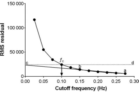
The application of the 10th order zero- lag low- pass Butterworth filter was conducted in the R environment32 using the signal package.33 The filter order was determined based on previous research,9,18 and the effects of filter order on the sharpness of filter response. The filters cutoff frequency (ƒc) was determined based on a combination of previous research,18 residual analysis (of data from three subjects) of the effects of a range of different normalized ƒc on HHb (Figure 1), and visual inspection with attention paid to local maxima and minima of filtered data compared to the raw signal.34 Based on these, it was concluded that 0.1 was suitable ƒc to be applied to the data for the remaining subjects. After the filter passed through the data, the resulting output was exported to Excel for standardization to occlusion values and determination of peaks and nadirs.
2.4
|
Data analysis
Six methods were used to obtain a single peak and nadir %Δ[HHb] value for every sprint and recovery period based on the methods outlined in previous research.8-12,18-22,29
1. Averages calculated from a predetermined range over the final 2 seconds of exercise (peak) and recovery (nadir): 2PD.
2. Averages calculated from a predetermined range over the final 5 seconds of exercise (peak) and recovery (nadir): 5PD.
3. Moving average with a window of 2 seconds applied to the data, followed by the identification peaks and nadirs within each 40-second exercise-recovery cycle: 2MA.
4. Moving average with a window of 5 seconds applied to the data, followed by the identification peaks and nadirs within each 40-second exercise-recovery cycle: 5MA
5. Application of a Butterworth filter to smooth the raw NIRS data, followed by the identification of peaks and na-dirs from predetermined time points. A single value prior to each phase change (ie, end of exercise and end of recov-ery, 0.1 second): BWFPD.
6. The application of a Butterworth filter to smooth the data, followed by the identification of a peak and nadir using a rolling approach within each 40-seconds exercise-recov-ery cycle (0.1 second): BWFMA.
Tissue reoxygenation (ΔReoxy) was calculated as the dif-ference between the peak and nadir for each analysis method.
2.5
|
Statistical analyses
Data in text and figures are presented as mean ± SD. Relative changes (%) are expressed with 95% confidence limits (95% CL). Effects of the Butterworth filter on the NIRS signal was assessed by calculating Pearson’s product- moment correla-tion (r), and standardized residuals of the raw vs filtered data in the R environment using the stats package.32 The correla-tion between the raw and filtered NIRS signal was assessed by fitting a linear regression model to the pooled subject data. The following criteria were adopted to interpret the magnitude of the correlation between variables: ≥0.1, trivial; >0.1- 0.3, small; >0.3- 0.5, moderate; >0.5- 0.7, large; >0.7- 0.9, very large; and >0.9- 1.0, almost perfect.35 To determine the effects FIGURE 1 A plot of the root- mean- square (RMS) residuals between filtered and unfiltered signals as a function of the filter cutoff frequency from the data of a representative subject. A line of best fit (ab) is projected to the Y- axis. At the intercept c, the horizontal line cd is drawn to intersect with the residuals. The chosen cutoff frequency ƒc
of analysis method, practical significance was also assessed by standardized effects and presented with 95% CL.36 Effect sizes (ES) between0- < 0.2, >0.2- 0.5, >0.5- 0.8, and >0.8 were con-sidered to as trivial, small, moderate, and large, respectively. Probabilities were also calculated to establish whether the chance the true (unknown) differences were lower, similar, or higher than the smallest worthwhile change (0.2 multiplied by the between- subject SD, based on Cohen’s effect size princi-ple). Quantitative probability of lower, similar, or higher dif-ferences was assessed qualitatively as follows: <1%, almost certainly not; >1%- 5%, very unlikely; >5%- 25%, unlikely; >25%- 75%, possible; >75%- 95%, likely; >95%- 99%, very likely; and >99%, almost certainly. If the probability of having higher/lower values than the smallest worthwhile difference was both >5%, the true difference was assessed as unclear.35,37 Data analysis was performed using a modified statistical Excel spreadsheet.38 To examine the interaction effects between the method for identifying Δ%[HHb] peak, nadir and ΔReoxy (predetermined and moving), and the size of the analysis window (0.1, 2, and 5 seconds), two- way repeated measure ANOVAs were performed. Post hoc analysis was conducted using the Holm- Šídák method and adjusted for multiple com-parisons. A threshold for significance was set at the P < .05 level. Analysis was performed GraphPad Prism 6.
3
|
RESULTS
3.1
|
Application of the Butterworth filter
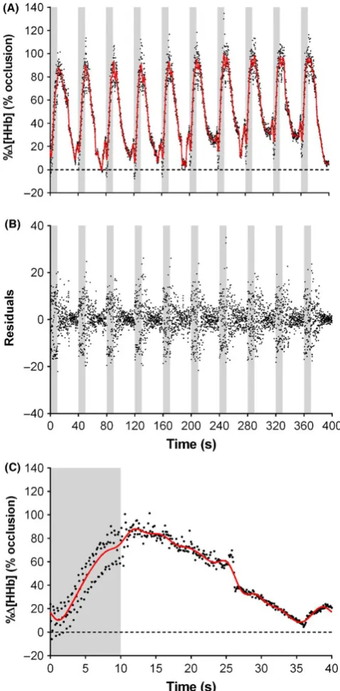
An example of the raw compared to the filtered data of a repre-sentative subject is presented in Figure 2. There was an almost perfect Pearson’s correlation between the raw NIRS data and that after the Butterworth filter (Figure 3A). The mean stand-ardized residual of the raw data compared to the filtered was - 9.71 × 10³ ± 3.80 (Figure 3B). When rectified, the mean re-sidual was 2.51 ± 2.86 with a relative difference of 2.5% [CL: 1.7, 3.4].3.2
|
Peak muscle [HHb]
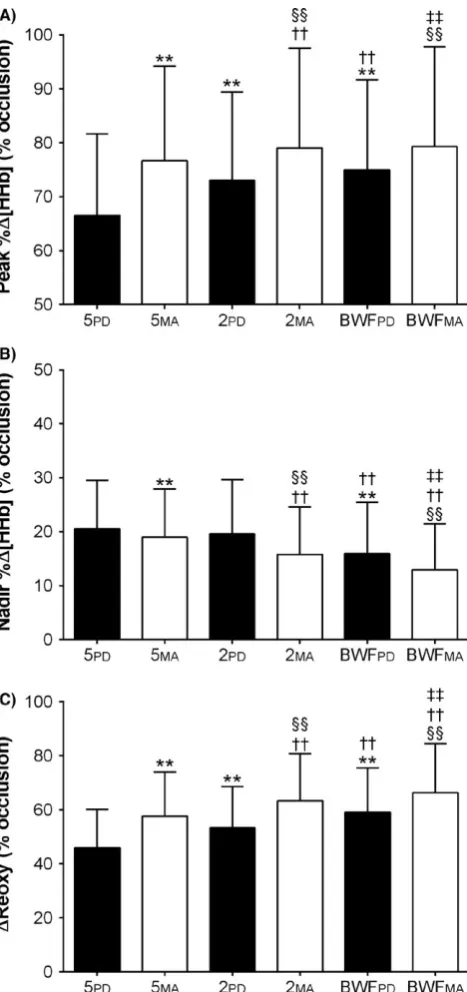
Mean results of the different analysis methods are presented in Figure 4A. Comparisons of analysis methods are shown in Table 1. There was a significant effect of the method for identify peaks on peak muscle Δ%[HHb] at the P < 0.05 level [F (1, 8) = 5.346, P = .0495]. The size of the analysis window also had a significant effect on peak muscle [HHb] [F (2, 16) = 29.68, P < .0001]. There was also a significant interaction effect [F (2, 16) = 6.445, P = .0089]. Changes in Δ%[HHb] across all sprints were almost certainly higher when calculated from 5MA compared to 5PD with a small effect (15.3% [11.7, 19.1]; P < .0001). There was also a likely small difference between 2MA and 2PD (8.2% [5.4, 11.0]; P < .0001). An almost certainly small effect was also observed when 2PD
an almost certainly trivial difference when compared to 2MA (0.4% [0.1, 0.7]; P = .4348). There was a likely trivial differ-ence between BWFMA and BWFPD.
3.3
|
Nadir muscle [HHb]
Mean results of the different analysis methods are presented in Figure 4B. Comparisons of analysis methods are shown in Table 2. A significant effect of the method for identify nadirs on peak muscle Δ%[HHb] was detected [F (1, 8) = 5.346, P = .0495]. The size of the analysis window also had a signifi-cant effect on nadir Δ%[HHb] [F (2, 16) = 29.68, P < .0001]. A significant interaction effect was also detected [F (2, 16) = 6.445, P = .0089]. The difference between 5MA and 5PD during recovery was trivial. However, a likely small differ-ence did exist between 2MA and 2PD (−19.7% [−33.8, −2.7]; P < .0001). A possibly small effect was also present when 2PD was compared to 5PD. There was a very likely small effect with 2MA being lower than 5MA. The BWFPD nadir was likely lower
than both 5PD and 2PD. Using BWFMA to calculate the nadir of Δ%[HHb] yielded very likely and likely lower means than 5MA (−40.4% [−58.1, −15.2]; P < .0001) and 2MA (−25.3% FIGURE 3 Correlation and residual analysis of the pooled
subject data comparing the output from the Butterworth filter to the raw deoxyhaemoglobin (HHb) data. (A) Pearson’s product- moment correlation (r) with associated P value of a linear regression model fitted to the filtered and raw HHb data. (B) Standardized residuals from the raw vs filtered data of the pooled subject data set
FIGURE 4 Mean and standard deviation of deoxyhaemoglobin concentration changes (Δ%[HHb]) over the entire repeated- sprint protocol determined from the different analysis methods. (A) Peak Δ%[HHb] averages of each analysis method. (B) Nadir Δ%[HHb] averages of each analysis method. (C) ΔReoxy calculated from peak and nadir Δ%[HHb] of the different analysis methods. The number of symbols one and two represent a difference at the P < 0.05 and
P < 0.01 level, respectively (Holm- Šídák test). Symbols denote a
difference from 5PD, *; 2PD, †; 5MA, §; BWFPD, ‡. No significant
difference was found between BWFMA – 2MA (P = 0.4348), and
[−39.5, −7.8]; P < .0001). Additionally, BWFMA was likely lower than BWFPD (−20.8% [−32.2, −7.4]; P < .0001).
3.4
|
Muscle reoxygenation
Mean results of the different analysis methods are presented in Figure 4C. Comparisons of analysis methods are shown in Table 3. There was a significant effect of the method for iden-tify peaks and nadirs on ΔReoxy [F (1, 8) = 40.00, P = .0002]. A significant effect of the window size was also detected [F (2, 16) = 108.9, P < .0001]. There was also a significant in-teraction effect [F (2, 16) = 13.31, P = .0004]. Using the 5MA method to calculate ΔReoxy yielded almost certainly higher results than 5PD (28.2% [17.7, 39.7]; P < .0001). Similarly, 2MA was very likely greater than 2PD (19.4 [11.2, 28.3]; P < .0001). Comparing the predetermined mean approaches, 2PD was very likely greater than 5PD. Rolling means were possibly higher when the 2MA approach was used compared to 5MA. When the Butterworth filter was used, values from predetermined time points (BWFpd) were almost certainly greater than 5PD (31.0% [22.4, 40.3]; P < .0001) and possibly greater than 2PD (10.9% [8.3, 13.5]; P < .0001). Means calculated from the BWFMA ap-proach were almost certainly higher than 5MA, almost certainly
trivial compared to 2MA, and likely greater than BWFPD (13.2% [7.9, 18.7]; P < .0001).
4
|
DISCUSSION
Results indicate that using predefined averaging windows to analyze the NIRS signal within sprint and recovery periods, Δ%[HHb] peaks and nadirs are consistently underestimated compared to a moving average, regardless of the window length. Subsequently, muscle reoxygenation between efforts is underes-timated using 5PD and 2PD compared to 5MA and 2MA. However, a drawback of using the arithmetic mean is that each data point contributes equally to the average, which allows outlying data points to bias the result.39 To overcome this, we applied a 10th order zero- lag low- pass Butterworth filter to the NIRS signal, which incorporates a weighted mean from several data points across the signal. Correlation and residual analysis revealed the Butterworth filter attenuated the “noise” yet maintained the in-tegrity of the raw data (Figure 3). As NIRS responses are used as a surrogate for metabolic perturbations, detecting the magni-tude of change is critical for assessing the influence of interven-tions and environmental factors. Thus, it appears that a digital filter combined with a rolling approach for determining peaks
Variable Analysis method comparison Standardized effect Relative difference (%)
Peak Δ%[HHb] (%) 2PD – 5PD 0.30 [0.34, 0.25] 9.8 [8.2, 11.4]
2MA – 5MA 0.09 [0.12, 0.06] 2.9 [3.9, 2.0]
5MA – 5PD 0.47 [0.57, 0.36] 15.3 [11.7, 19.1]
2MA – 2PD 0.25 [0.33, 0.17] 8.2 [5.4,11.0]
BWFPD – 5PD 0.40 [0.47, 0.32] 12.9 [10.4, 15.5]
BWFPD – 2PD 0.09 [0.13, 0.06] 2.9 [1.7, 4.0]
BWFMA – 5MA 0.56 [0.66, 0.46] 19.2 [15.4, 23.1]
BWFMA – 2MA 0.01 [0.02, 0.00] 0.4 [0.1, 0.7]
BWFMA – BWFPD 0.17 [0.25, 0.10] 5.6 [3.0, 8.1]
Standardized effects and relative differences are presented as change score [95% confidence limits].
TABLE 1 Comparison of smoothing method responses on peak Δ%[HHb]
Variable Analysis method comparison Standardized effect Relative difference (%)
Nadir Δ%[HHb]
(%) 2PD- 5PD −0.20 [0.18, −0.59] −8.9 [−23.5, 8.6] 2MA- 5MA −0.38 [−0.13, −0.64] −20.3 [−31.4, −7.3]
5MA- 5PD −0.19 [0.04, −0.42] −8.3 [−17.6, 1.8]
2MA- 2PD −0.37 [−0.05, −0.70] −19.7 [−33.8, −2.7]
BWFPD- 5PD −0.47 [−0.10, −0.84] −31.0 [−48.5, −7.5]
BWFPD- 2PD −0.35 [−0.15, −0.55] −24.3 [−35.3, −11.5]
BWFMA- 5MA −0.61 [−0.19, −1.02] −40.4 [−58.1, −15.2]
BWFMA- 2MA −0.34 [−0.10, −0.59] −25.3 [−39.5, −7.8]
BWFMA- BWFPD −0.27 [−0.09, −0.46] −20.8 [−32.2, −7.4]
Standardized effects and relative differences are presented as change score [95% confidence limits].
and nadirs of the NIRS signal is the best method for accurate interpretation of oxygenation trends in repeated- sprint exercise.
There were clear differences in peak Δ%[HHb] means tween the predefined averaging methods. The difference be-tween 2PD and 5PD can be attributed to the length of the averaging window. At sprint onset, there is a sharp rise in Δ%[HHb] from rest that peaks at sprint cessation or shortly thereafter (Figure 2 and Ref. [8,10,12,13,18]). In our representative data, Δ%[HHb] continued to increase ~40% in the final 5 s of the first sprint which led to a significant 10% reduction in peak Δ%[HHb] for 5PD compared with 2PD (Table 1). Consequently, an averaging duration that encapsulates a sharp rise within the window length will underestimate the amplitude of Δ%[HHb] change.
It is clear from Figure 2 that Δ%[HHb] continued to increase after the predefined averaging window. This would tend to under-estimate the peak Δ%[HHb] response. To overcome this potential confounding factor, we applied both a 5- second and 2- second mov-ing average to the NIRS signal. The 2MA and 5MA yielded 15% and 8% greater peaks compared to 2PD and 5PD, respectively. As maxi-mal Δ%[HHb] may occur either at, or immediately after sprint ces-sation, identification of peaks using a moving average will always capture this maximal deoxygenation. Therefore, studies that only employed predetermined averaging windows9,11,17,20-22 may have underestimated the true magnitude of Δ%[HHb] change induced by repeated- sprint exercise. To more accurately represent muscle oxygenation changes in response to repeated- sprint exercise, values need to be determined from a moving average approach.8,10,12,18,19,29 However, a moving average may not be appropriate when exercise protocols incorporate other muscular activity around repeated- sprint bouts. For example, some authors have used low- intensity exercise during recovery periods between sprints,8,10,12 and oth-ers have used running- based protocols, which impose eccentric loading during the negative acceleration phase post- sprint.8,14,17 Another limitation is that when using arithmetic means (ie, 5PD and 2PD; 5MA and 2MA), equal weight is given to all data points, which can lead to the result being distorted by outliers.39 But in the field of repeated- sprint exercise, an arithmetic mean is commonly em-ployed to smooth perturbations in NIRS data.
To address this methodological limitation, we used a Butterworth filter to smooth the data and obtained Δ%[HHb] peak from both predetermined time points within each sprint and from a rolling approach. The BWFPD approach yielded 13 and 3% greater peaks than both 5PD and 2PD methods, respectively. As BWFPD used the last value within each sprint (in the current instance, the 100th value of a 10- second sprint sampled at 10 Hz), this was the highest Δ%[HHb] value achieved within each 10- second sprint period. Similarly, peak Δ%[HHb] determined by BWFMA was 19% greater than 5MA. However, only a trivial difference was found between BWFMA filtering and 2MA. Various studies have applied digital filters to smooth biomechanical and biological data,34,40,41 and yet few authors have used a filter to smooth a NIRS signal during repeated- sprint exercise.9,18 When a low- pass filter is used, a ƒc is chosen so that lower signal fre-quencies remain and higher frefre-quencies (noise) are attenuated.28 A low- pass Butterworth filter attenuates signal power above a specified ƒc, but also included a weighted average across several data points,27 which leads to lag in the signal output. This tempo-ral shift can be removed by running the filter a second time in the reverse direction (zero- lag). Repeated- sprint exercise represents a particularly salient challenge to Δ%[HHb] signal due to the rapid changes in duty cycle. Our results suggest that an arithmetic mean under- represents [HHb] peak in most cases and that both BWFPD and BWFMA better reflect peak [HHb] after sprint exercise.
Differences in nadir Δ%[HHb] were less clear between the averaging methods. As means were calculated on the flatter portion of the NIRS signal during the late stage of recovery, differences between averaging methods were minimal. There was an 8% and 20% lower Δ%[HHb] nadir from both a 5MA and 2MA compared to 5PD and 2PD, respectively (Table 2). While the difference between nadir 5MA and 5PD did not reach the typ-ically adopted threshold for statistical significance of P < .05 (“trivial” standardized effect), we reported a small standardized effect (20% relative difference, P < .0001) between the 2MA and 2PD analysis methods. The 5- s averaging windows may not have the sensitivity to detect subtle differences between the nadir determined from predetermined and moving averages. It
Variable Analysis method comparison Standardized effect Relative difference (%)
ΔReoxy (%) 2PD- 5PD 0.34 [0.48, 0.20] 18.2 [10.1, 26.9]
2MA- 5MA 0.21 [0.26, 0.17] 10.1 [7.9, 12.3]
5MA- 5PD 0.52 [0.71, 0.34] 28.2 [17.7, 39.7]
2MA- 2PD 0.39 [0.55, 0.23] 19.4 [11.2, 28.3]
BWFPD- 5PD 0.56 [0.70, 0.42] 31.0 [22.4, 40.3]
BWFPD- 2PD 0.21 [0.26, 0.16] 10.9 [8.3, 13.5]
BWFMA- 5MA 0.32 [0.39, 0.26] 15.7 [12.5, 18.9]
BWFMA- 2MA 0.11 [0.14, 0.08] 5.1 [3.5, 6.7]
BWFMA- BWFPD 0.28 [0.38, 0.17] 13.2 [7.9, 18.7]
Standardized effects and relative differences are presented as change score [95% confidence limits].
appears that a short moving average is better suited at detecting changes in nadir Δ%[HHb]. As the restoration of NIRS variable toward baseline has become a surrogate for metabolic recovery between sprints,8,10,11,15,17 an accurate depiction of this variable is necessary to assess metabolic perturbations leading to greater peripheral fatigue. Additionally, the detection of the magnitude of change has important implications for assessing the potency of training programs and environmental factors. Unless the nadir of the signal is obtained from a rolling approach, the mag-nitude of [HHb] recovery will be underestimated.
The ΔReoxy is determined from both peak and nadir Δ%[HHb] responses, and hence, the analysis method that yields the greatest peaks and nadirs will have the greatest ΔReoxy. Consequently, we observed clear and substantial differences between all ΔReoxy analysis methods apart from BWFMA vs 2MA, with a range of rel-ative differences from 5% to 31%. Studies reporting ΔReoxy from predetermined windows11,17 have likely underestimated reoxy-genation capacity. The most accurate representation of ΔReoxy would come from works that have chosen a moving average ap-proach for the determination of peaks and nadirs.12,18
Irrespective of the method, a narrow window for analysis (2 seconds) allows reporting greater magnitudes of response than a longer window (5 seconds). However, care should be taken when using a narrow analysis window. It contains less data from which the average is calculated, which increases the risk that outliers bias the calculated mean.39 Such a method-ological pitfall is displayed in the sprint phase of Figure 2A, where a small number of data points are far above the charac-teristics of the surrounding data. A narrow analysis window would place greater weight on these individual data points in the mean compared to a larger window.39 Currently, there is no consistency on the length of the analysis window. In some cases, a window as large as 5 seconds8,11,21,22 and as small as 1 seconds10,12 has been used. When a Butterworth filter was employed, both peak and nadir values18 and a 2- second aver-age9 have been used. However, using a Butterworth filter, a single data point from the resulting output can be used with assurance that it reflects the characteristics of the surround-ing data. Although our choice to use a Butterworth filter was based on previous research,9,18,29 other smoothing/filtering techniques which eliminate outliers may also yield similar re-sults. Readers should also be aware that these data and ana-lytical methods were collected during isokinetic sprints where cadence was constrained to 120 rpm, and, although muscle ox-ygenation patterns appear similar, one may exert caution when analyzing NIRS signal in nonisokinetic conditions where ca-dence is influenced by gear ratio and neuromuscular fatigue.
5
|
PERSPECTIVE
NIRS- derived variables in sprint exercise are subject to rapid and large perturbations. Furthermore, during cyclic movements
such as running or cycling, there are relatively large oscillations in the [HHb] signal response due to mechanical effects of mus-cle contraction on local blood flow. This requires appropriate smoothing of the signal to avoid either over or underestimation of peaks and nadirs. Sprint and recovery means calculated over a 1- 5 seconds window in predetermined time frames are often reported,8,9,11,13,14,17,20–25 however, there remains little consist-ency between studies examining muscle oxygenation during repeated- sprint exercise. The current results reveal that mov-ing averages derive greater changes in muscle oxygenation than means calculated from predetermined time points. Hence, this method is less prone to underestimation of the maximum rate of de- and reoxygenation. However, as these calculations are susceptible to signal bias from outliers, especially when a shorter averaging window is used,39 we recommend using a digital filter9,18,29 or other smoothing/filtering techniques prior to analysis. We also suggest that future studies should avoid pre-determined analysis windows and focus on the determination of a single value for peaks and nadirs from a rolling approach.
ACKNOWLEDGMENTS
We would like to thank those who assisted with data collection and pilot testing; Kristal Hammond, Andrew Hibbert, Samuel Howe, Mathew Inness, Michele Lo, Briar Rudsits, and Alice Sweeting. We would also like to thank the laboratory technical staff; Samantha Cassar, Jessica Meilak, and Collene Steward.
CONFLICT OF INTEREST
No authors had a conflict of interest regarding any aspect of the research.
AUTHOR CONTRIBUTIONS
RFR, NET, RJA, and FB conceptualized and designed the research project; RFR acquired the data and conducted the statistical analysis; RFR interpreted results with assistance from NET, RJA, and FB; RFR wrote the manuscript with revisions from NET, RJA, and FB. All authors reviewed and agreed upon the final manuscript.
ORCID
R. F. Rodriguez http://orcid.org/0000-0001-5806-7652
N. E. Townsend http://orcid.org/0000-0002-2328-4638
REFERENCES
2. Grassi B, Pogliaghi S, Rampichini S, et al. Muscle oxygenation and pulmonary gas exchange kinetics during cycling exercise on- transitions in humans. J Appl Physiol. 2003;95:149‐158. 3. De Blasi RA, Cope M, Elwell C, Safoue F, Ferrari M. Noninvasive
measurement of human forearm oxygen consumption by near in-frared spectroscopy. Eur J Appl Physiol. 1993;67:20‐25. 4. Ferrari M, Muthalib M, Quaresima V. The use of near- infrared
spec-troscopy in understanding skeletal muscle physiology: recent devel-opments. Philos Trans A Math Phys Eng Sci. 1955;2011:4577‐4590. 5. McLay KM, Fontana FY, Nederveen JP, et al. Vascular respon-siveness determined by near- infrared spectroscopy measures of oxygen saturation. Exp Physiol. 2016;101:34‐40.
6. Ferrari M, Quaresima V. A brief review on the history of human functional near- infrared spectroscopy (fNIRS) development and fields of application. NeuroImage. 2012;63:921‐935.
7. Ferrari M, Mottola L, Quaresima V. Principles, techniques, and limitations of near infrared spectroscopy. Can J Appl
Physiol. 2004;29:463‐487.
8. Buchheit M, Cormie P, Abbiss CR, Ahmaidi S, Nosaka KK, Laursen PB. Muscle deoxygenation during repeated sprint running: effect of active vs. passive recovery. Int J Sports Med. 2009;30:418‐425. 9. Sandbakk Ø, Skalvik TF, Spencer M, et al. The physiological
re-sponses to repeated upper- body sprint exercise in highly trained athletes. Eur J Appl Physiol. 2015;115:1381‐1391.
10. Ohya T, Aramaki Y, Kitagawa K. Effect of duration of active or pas-sive recovery on performance and muscle oxygenation during inter-mittent sprint cycling exercise. Int J Sports Med. 2013;34:616‐622. 11. Billaut F, Buchheit M. Repeated- sprint performance and vastus
lateralis oxygenation: effect of limited O2 availability. Scand J
Med Sci Sports. 2013;23:185‐193.
12. Ohya T, Hagiwara M, Suzuki Y. Inspiratory muscle warm- up has no impact on performance or locomotor muscle oxygen-ation during high- intensity intermittent sprint cycling exercise.
SpringerPlus. 2015;4:1‐11.
13. Racinais S, Bishop DJ, Denis R, Lattier G, Mendez-Villaneuva A, Perrey S. Muscle deoxygenation and neural drive to the muscle during repeated sprint cycling. Med Sci Sports Exerc. 2007;39:268‐274. 14. Galvin HM, Cooke K, Sumners DP, Mileva KN, Bowtell JL.
Repeated sprint training in normobaric hypoxia. Br J Sports
Med. 2013;47(Suppl 1):i74‐i79.
15. Bowtell JL, Cooke K, Turner R, Mileva KN, Sumners DP. Acute physiological and performance responses to repeated sprints in varying degrees of hypoxia. J Sci Med Sport. 2014;17:399‐403. 16. Takaishi T, Sugiura T, Katayama K, et al. Changes in blood
vol-ume and oxygenation level in a working muscle during a crank cycle. Med Sci Sports Exerc. 2002;34:520‐528.
17. Buchheit M, Ufland P. Effect of endurance training on perfor-mance and muscle reoxygenation rate during repeated- sprint run-ning. Eur J Appl Physiol. 2011;111:293‐301.
18. Faiss R, Leger B, Vesin JM, et al. Significant molecular and sys-temic adaptations after repeated sprint training in hypoxia. PLoS
ONE. 2013;8:e56522.
19. Jones B, Hamilton DK, Cooper CE. Muscle oxygen changes fol-lowing sprint interval cycling training in elite field hockey play-ers. PLoS ONE. 2015;10:e0120338.
20. Billaut F, Kerris JP, Rodriguez RF, Martin DT, Gore CJ, Bishop DJ. Interaction of central and peripheral factors during repeated sprints at different levels of arterial O2 saturation. PLoS ONE. 2013;8:e77297. 21. Smith KJ, Billaut F. Influence of cerebral and muscle oxygenation
on repeated- sprint ability. Eur J Appl Physiol. 2010;109:989‐999.
22. Smith KJ, Billaut F. Tissue oxygenation in men and women during repeated- sprint exercise. Int J Sports Physiol Perform. 2012;7:59‐67. 23. Dupont G, Moalla W, Guinhouya C, Ahmaidi S, Berthoin S.
Passive versus active recovery during high- intensity intermittent exercises. Med Sci Sports Exerc. 2004;36:302‐308.
24. Cheng CF, Tong TK, Kuo YC, Chen PH, Huang HW, Lee CL. Inspiratory muscle warm- up attenuates muscle deoxygenation during cycling exer-cise in women athletes. Respir Physiol Neurobiol. 2013;186:296‐302. 25. Buchheit M, Hader K, Mendez-Villanueva A. Tolerance to high-
intensity intermittent running exercise: do oxygen uptake kinetics really matter? Front Physiol. 2012;3:406.
26. Ihsan M, Abbiss CR, Lipski M, Buchheit M, Watson G. Muscle oxygenation and blood volume reliability during continuous and intermittent running. Int J Sports Med. 2013;34:637‐645. 27. Elmer SJ, Martin JC. Fourier series approximations and low pass
filtering: facilitating learning of digital signal processing for bio-mechanics students. Sportscience. 2009;13:1‐8.
28. Yu B, Gabriel D, Noble L, An KN. Estimate of the optimum cut-off frequency for the Butterworth low- pass digital filter. J Appl
Biomech. 1999;15:318‐329.
29. Willis SJ, Alvarez L, Millet GP, Borrani F. Changes in muscle and cerebral deoxygenation and perfusion during repeated sprints in hypoxia to exhaustion. Front Physiol. 2017;8:846.
30. van Soest AJ, Casius LJ. Which factors determine the optimal pedal-ing rate in sprint cyclpedal-ing? Med Sci Sports Exerc. 2000;32:1927‐1934. 31. Gotshall RW, Bauer TA, Fahrner SL. Cycling cadence alters
exer-cise hemodynamics. Int J Sports Med. 1996;17:17‐21.
32. R Foundation for Statistical Computing. R: a language and
environ-ment for statistical computing [computer program]. Version 1.0.136.
Vienna, Austria: R Foundation for Statistical Computing; 2016. 33. Signal Developers. Signal: Signal processing [computer program].
Version 0.7-6: R Foundation for Statistical Computing; 2013.
34. Winter DA. Biomechanics and motor control of human
move-ment. 4th edn. New Jersey: John Wiley & Sons; 2009.
35. Hopkins WG, Marshall SW, Batterham AM, Hanin J. Progressive statistics for studies in sports medicine and exercise science. Med Sci
Sports Exerc. 2009;41:3‐13.
36. Cohen J. Statistical power analysis for the behavioral sciences. Routledge; 1988.
37. Batterham AM, Hopkins WG. Making meaningful inferences about magnitudes. Int J Sports Physiol Perform. 2006;1:50‐57. 38. Hopkins WG. Spreadsheets for analysis of controlled trials, with
ad-justment for a subject characteristic. Sportscience. 2006;10:46‐50. 39. Dawson B, Trapp RG. Basic and clinical biostatistics, 4th edn.
New York: Lange Medical Books/McGraw-Hill; 2004.
40. Robertson DG, Dowling JJ. Design and responses of Butterworth and critically damped digital filters. J Electromyogr Kinesiol. 2003;13:569‐573.
41. Schlichthärle D. Digital filters. basics and design. 2nd ed. Berlin; Heidelberg; New York: Springer; 2011.
How to cite this article: Rodriguez RF, Townsend NE, Aughey RJ, Billaut F. Influence of averaging method on muscle deoxygenation interpretation during repeated-sprint exercise. Scand J Med Sci Sports. 2018;28:2263– 2271.
![TABLE 2 method responses on nadir Δ%[HHb]](https://thumb-us.123doks.com/thumbv2/123dok_us/7964906.1321096/6.595.52.381.240.411/table-method-responses-on-nadir-d-hhb.webp)
