RESEARCH ARTICLE A Study on Image Restoration and its Various Blind Image Deconvolution Algorithms

(1)

International Journal of Computer Science and Mobile Computing

A Monthly Journal of Computer Science and Information Technology

ISSN 2320–088X

IJCSMC, Vol. 2, Issue. 10, October 2013, pg.273 – 278

RESEARCH ARTICLE

A Study on Image Restoration and its Various

Blind Image Deconvolution Algorithms

P. Jayapriya1, Dr. R. Manicka Chezhian2 jayapriyapalanisamy@yahoo.co.in, chezian_r@yahoo.co.in

1Research Scholar, Dr. Mahalingam Centre for Research and Development (CS), NGM College, TamilNadu, India

2

Associate Professor, Dr. Mahalingam Centre for Research and Development (CS), NGM College, TamilNadu, India

Abstract

Motion blur is an inevitable tradeoff between the amount of blur and the amount of noise in the acquired images. The effectiveness of any restoration algorithm typically depends on these amounts, and it is difficult to find their best balance in order to ease the restoration task. While the Point-Spread-Function (PSF) trajectories as random processes, expresses the restoration performance. The expectation of the restoration error is conditioned on some motion-randomness descriptors and the exposure time. By using blind deconvolution algorithms with estimated PSF on single-image; blur kernel is directly estimated from light streaks in the blurred image. Combining with the sparsity constraint, blind de-convolution algorithms and maximum likelihood estimation approach, it can be solved quickly and accurately from a user input image. This blind kernel (PSF) can then be applied to single-image to restore the sharp image. This paper describes the concept of Image Restoration and Blind Deconvolution Algorithms with various images.

Keywords: Image Restoration; Image Degradation; Deconvolution; Blind Image Deconvolution; Point Spread Function (PSF)

I. INTRODUCTION

(2)

camera motion, random atmospheric turbulence, Others. In most of the existing image restoration methods, the degradation process can be described using a mathematical model. A simplified version for the image restoration process model is:

y (i, j ) = H [f (i, j )]+ n(i, j), where

y(i, j) The degraded image

f (i, j) The original image H An operator that represents the degradation process.

n(i, j) The external noise which is assumed to be image-independent.

II. IMAGE RESTORATION

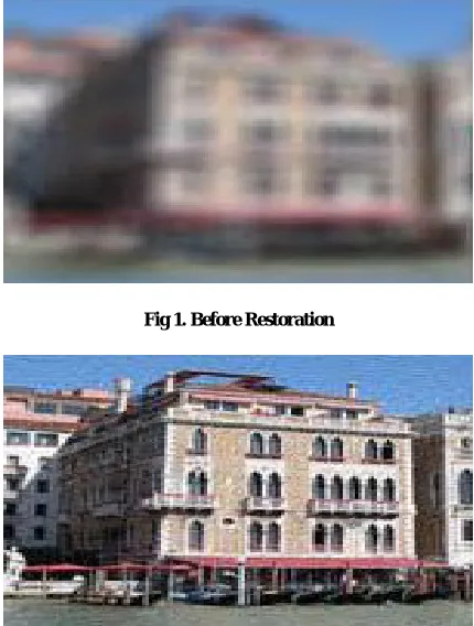
The purpose of image restoration is to compensate defects which help to degrade an image. In cases like motion blur, it is possible to come up with a very good estimate of the actual blurring function and remove the blur to restore the original image. In cases when the image is corrupted by noise, the best is to compensate for the degradation it caused. [2]

Fig 1. Before Restoration

Fig 2 After Restoration

(3)

Essentially, it tries to perform an operation on the image that is the inverse of the imperfections in the image formation system. In the use of image restoration methods, the characteristics of the degrading system and the noise are assumed to be known a priori. In practical situations, however, one may not be able to obtain this information directly from the image formation process. The goal of blur identification is to estimate the attributes of the imperfect imaging system from the observed degraded image itself prior to the restoration process. The combination of image restoration and blur identification is often referred to as blind image deconvolution [3].

III. ANALYSIS ON BLIND IMAGE DECONVOLUTION

Blind deconvolution is the problem of recovering a sharp version of an input blurry image when the blur kernel is unknown [2]. By decomposing a blurred image y it can be represented as

y = k ! x where

x is a visually plausible sharp image, and k is a nonnegative blur kernel.

Deconvolution is a longstanding problem in many areas of signal and image processing (e.g., biomedical imaging

astronomy, and remote-sensing, to quote a few). For example, research in astronomical image deconvolution has recently seen considerable work, partly triggered by the Hubble space telescope (HST) optical aberration problem at the beginning of its mission. In biomedical imaging, researchers are also increasingly relying on deconvolution to improve the Quality of images acquired by confocal microscopes [4]. Deconvolution may then

prove crucial for exploiting images and extracting scientific content.

IV LITERATURE REVIEW ON BLIND IMAGE DECONVOLUTION ALGORITHMS

There are various filtering methods available to reduce noise and blurring, but it has its own disadvantage, and then developed various Deconvolution algorithms.

D. A. Fish et. al have presented a blind deconvolution algorithm based on the Richardson–Lucy deconvolution algorithm. It is developed from Baye’s theorem. It has been used extensively in many applications because it is adapted to Poisson noise. In this algorithm initial guess is required for the object to start algorithm. Then after that in subsequent iteration large deviation in the guess from true object are lost rapidly in initial iteration whereas detail is added more slowly in subsequent iteration. Two iterations are performed within blind iteration, one for object evaluation and one for PSF evaluation [1]. Advantages of this algorithm include a nonnegative constraint if the initial guess f0(x) H0 in which energy is conserved as the iteration proceeds.

Jae Myung have proposed maximum likelihood estimation approach, which is originally developed by R.A. Fisher in 1920, states that desired probability distribution is the one that makes the observed data most likely[6]. Estimation of parameter is made such that the probability or likelihood of receiving the observed image given the parameter set is maximized. Benefit of this approach is to estimate the true image that is produced at every iteration and the algorithm is easily terminated when result is obtained [7].

(4)

to the corrupted one and image model give relation between currently processed pixel and those already restored. Restoration is obtained by recombining all restoration components. Advantage is avoiding heavy computational load [8].

S. Derin Babacan have presented algorithm for total variation (TV) based blind deconvolution and parameter estimation utilizing variational framework. In this, blind deconvolution method has been implemented where unknown image, blur, and Hyper parameters are estimated simultaneously. Unknown parameters can be of Bayesian formulation can be calculated automatically using only observation or using also prior knowledge with different confidence values to improve performance of algorithm. It gives higher quality restoration in both synthetic and real image experiment [3].

Feng-qing Qin has proposed method of blind image super-resolution reconstruction. The point spread function of the imaging system is estimated to approximate the low resolution imaging process much more accurately. Utilizing Wiener filtering image restoration algorithm, multiple error parameter curves are generated at different parameters. The super resolution reconstructed image has higher spatial resolution and better visual effect [5].

V.POINT SPREAD FUNCTION (PSF)

Most blurring processes can be approximated by convolution integrals, also known as Fredholm integral equations. The blurring is characterized by a Point-Spread Function (PSF) or impulse response. The PSF is the output of the imaging system for an input point source. All the blurring processes considered in this paper are linear and have a spatially invariant PSF [10].

For discrete image processing, the convolution integral is replaced by a sum. The blurry image x(n, m) is obtained from the original image s(n, m) by this convolution:

The function h(n, m) is the discrete Point Spread Function for the imaging system. Also of interest is the Discrete Fourier Transform (DFT) representation of the point-spread function, given by:

(5)

5.1 PSF GENERATION

The PSFs constituting the collections HT, which are used to compute the restoration-error models, are obtained

by sampling continuous trajectories on a (regular) pixel grid. Each trajectory consists of the positions of a particle following a 2-D random motion in continuous domain. The particle has an initial velocity vector with each iteration is affected by a Gaussian perturbation and by a deterministic inertial component, directed toward the current particle position. In addition, with a small probability, an impulsive perturbation aiming at inverting the particle velocity arises, mimicking a sudden movement that occurs when the user presses the camera button or tries to compensate the camera shakes.

At each step, the velocity is normalized to guarantee that trajectories corresponding to equal exposures have the same length. Each perturbation (Gaussian, inertial, and impulsive) is ruled by its own parameter, and each set

HT contains PSFs sampled from trajectories generated by parameters spanning a meaningful range of values.

Rectilinear trajectories are generated when all the perturbation parameters are zero.

Each PSF hT ∈ HT consists in discrete values that are computed by sampling a trajectory on a regular pixel

grid, using sub-pixel linear interpolation. Collections corresponding to different exposure times are obtained by scaling the values of each PSF by a constant factor.

Recollect that Image restoration refers to the removal or minimization of known degradations in an image. This includes de-blurring of images degraded by the limitations of the sensor or its environment, noise filtering, and correction of geometric distortions or non-linearities due to sensors. It describes the imaging system response to a point input, and is analogous to the impulse response. A point input, represented as a single pixel in the “ideal” image, will be reproduced as something other than a single pixel in the “real” image.

“Point Spread Functions” describe the two-dimensional distribution of light in the telescope focal plane for

astronomical point sources. Modern optical designers put a great deal of effort into reducing the size of the PSF for large telescopes.

(6)

which are equipped with “active” or “adaptive” optics systems, which can greatly reduce the effects s of atmospheric seeing on the PSF.

VI. CONCLUSION

Restoration technology of image is one of the important technical areas in image processing. In this paper various blind image restoration techniques have been discussed. Methods are based on blind deconvolution approach with partial information available about true image. Advantage of using blind deconvolution algorithm based on Richardson–Lucy deconvolution algorithm is to de-blur the degraded image with prior knowledge of PSF and Poisson noise whereas other algorithms concentrate on the Gaussian noise. Better restoration can be achieved by estimating the PSF, as this approach does not require verification of the blur kernel against the blurred image, the de-blurring can be performed quickly enough for interactive use.

REFERENCES

[1] D. A. Fish, A. M. Brinicombe, and E. R. Pike, “Blind deconvolution by means of the Richardson–Lucy algorithm,” J. Opt. Soc. Am. A/Vol. 12, No. 1/January 1995

[2] Deepa Kundur and Dlmltrlos Hatzinakos, “Blind image deconvolution,” IEEE Signal Processing magazine, vol. 13 (3), pp. 43-64, May 1996.

[3] S. Derin Babacan, “Variational Bayesian Blind Deconvolution Using a Total Variation Prior”, IEEE Transactions on Image Processing, Vol. 18, No.1, January 2009

[4] Esmaeil Faramarzi, Dinesh Rajan, Marc P. Christensen,“Unified Blind Method for Multi-Image Super-Resolution and Single/Multi-Image Blur Deconvolution”, IEEE transactions on Image Processing, vol. 22, no. 6, pp: 2101-2105, June 2013.

[5] Feng-qing Qin, “Blind Image Super-Resolution Reconstruction based on PSF estimation”, Proceedings of the IEEE International Conference on Information and Automation, Harbin, China., June 20 - 23, 2010.

[6]In Jae Myung”,Tutorial on maximum likehood estimation,”OH 43210-1222,USA Received 30 November 2001,revised 15 October 2002

[7]Giacomo Boracchi and Alessandro Foi, “Modeling the Performance of Image Restoration from Motion Blur” IEEE transactions on Image Processing, vol. 21 No. 8, pp.3502-3506, August 2012

[8]M.Mattavelli, G.Thonet, V.Vaerman, B.Macq, “Image restoration by 1D Kalman Filtering on Oriented Image Decompositions”, IEEE 1996

[9] Rafael C. Gonzalez, Richard E. Woods, “Digital Image processing”, 2nd ed., Prentice Hall, NJ.pp.1-20,221-227 2002.