What is Assumed in the GTAP Database's Disaggregation of Labor by Skill Level?

Full text

(1)CENTRE of POLICY STUDIESand the IMPACT PROJECT. Eleventh Floor Menzies Building Monash University Wellington Road CLAYTON Vic 3800 AUSTRALIA Telephone: (03) 9905 2398, (03) 9905 5112. from overseas: 61 3 9905 2398 61 3 9905 5112 61 3 9905 2426. Fax : (03) 9905 2426 e-mail web site:. [email protected] http://www.monash.edu.au/policy/. WHAT IS ASSUMED IN THE GTAP DATABASE’S DISAGGREGATION OF LABOR BY SKILL LEVEL? by. Gouranga Gopal DAS. Centre of Policy Studies and Department of Economics Monash University. Preliminary Working Paper No. IP-75 October 1999. ISSN 1031 9034. ISBN 0 7326 1518 6. The Centre of Policy Studies is a research centre at Monash University devoted to quantitative analysis of issues relevant to Australian economic policy..

(2) WHAT IS ASSUMED IN THE GTAP DATABASE’S DISAGGREGATION OF LABOR BY SKILL LEVEL?. by. Gouranga Gopal DAS Department of Economics/Centre of Policy Studies, Monash University, Clayton, Melbourne, Victoria-3168, Australia E-mail: [email protected]. ABSTRACT The 45 region × 50 commodity × 5 primary factor version of the GTAP database provides us with the splits of total labor payments into two categories, viz. skilled and unskilled labor in each sector. The decomposition of total labor payments in all sectors and all regions according to differentials in the skill content of the labor force presupposes substitution possibilities between these two categories of labor. Our interest is to explore the elasticity of substitution implicit in this disaggregation of occupation types. Given the skilled labor payment shares (as calculated from the GTAP database), we offer an ex post rationalization of them within a production-theoretic framework, thereby deriving estimates of the elasticity of substitution between skilled and unskilled labor. The adoption of a suitable nesting of skilled and unskilled labor in GTAP’s production function enables us to find a ‘reasonable’ value for the substitution elasticity that is implicit between the two categories of labor in the GTAP database. This relies on the inter-regional covariation in the GTAP shares and in measures of educational attainment. JEL classification: J24, J31, O15. Keywords: Elasticity of substitution; Educational attainment; Skilled and unskilled labor payment.. i.

(3) CONTENTS ABSTRACT. i. 1. Introduction. 1. 2. GTAP Methodology. 2. 3. Data Reviews and Reconciliation. 3. 3.1 Barro-Lee Dataset 3.2 DNS Dataset 3.3 Reconciliation of GTAP Database and DNS (1995) Database: 3.4 Reconciliation of GTAP Database and BL (1996) Database: 4. From Empirics to Theory. 3 3 5 8 11. 4.a. Production Nest 4.b. Estimation Procedure. 11 13. 5. Estimation Results. 14. 6. Summary. 16. REFERENCES. 18. LIST OF TABLES Table 1: Table A1: Table A2: Table A3: Table A4: Table A5: Table A6:. Table A7:. Table A8:. Elasticity of substitution regressions excluding GTAP composite regions Skilled labor payment shares in GTAP sectors and reg ions Mean years of education per working person and skill ed labor payment shares for all GTAP regions Skilled labor payment shares and mean school years of education for selected GTAP regions Skilled labor payment shares and mean years of tertiary education for selected GTAP regions Skilled labor payment shares, average years of higher and total schooling for selected GTAP regions Mean school years of education per working person (DNS database) and skilled labour payment shares for single GTAP regions Mean school years of education per working person (BL database) and skilled labour payment shares for single GTAP regions Elasticities of substitution regressions including GTAP composite regions. 16 19 24 25 26 27. 28. 29 30. LIST OF FIGURES Figure Figure Figure Figure Figure Figure. 1: 2: 3: 4: 5: 6:. Scatter-plot of SKL_AC and MEDY_AC and fitted regression Scatter-plot of SKL_AC and MTRY_AC and fitted regression Scatter-plot of SKL_AC and TYR_BL and fitted regression Scatter-plot of SKL_AC and HYR_BL and fitted regression Comparison between the regression lines A Production tree for GTAP incorporating human capital. ii. 6 7 9 9 10 12.

(4) WHAT IS ASSUMED IN THE GTAP DATABASE’S DISAGGREGATION OF LABOR BY SKILL LEVEL?# 1 Introduction The 45 region × 50 commodity × 5 primary factor version of the GTAP database provides us with the splits of total labor payments into two categories, viz. skilled and unskilled labor (in terms of the ILO one-digit classification of workers by occupation) in each sector. 1 The aggregate labor force going into the production process is, thus, classified into ‘raw’ labor and specialised ‘skilled’ labor. The decomposition of total labor payments in all sectors and all regions according to differentials in the skill content of the labor force presupposes substitution possibilities between these two categories of labor. Our interest is to explore the elasticity of substitution implicit in this disaggregation of occupation types2. As will be evident from our analysis, the adoption of a suitable nesting of skilled and unskilled labor in GTAP’s production function enables us to find a ‘reasonable’ value for the substitution elasticity that is implicit between the two categories of labor in the GTAP database. To do this, in Section 2 we describe the GTAP methodology, while Section 3 reviews available data sources on educational attainment and reconciles them with the GTAP data base. Section 4 offers some theoretical underpinning to the basis of our empirical analysis. Section 5 reports the results.. Concluding. remarks are offered in Section 6.. #. 1 2. This short paper is an abridged version of a paper titled “Educational attainment, skilled labor payment and absorption capacity: Empirics and Theory” which forms part of my PhD thesis in progress. I gratefully thank my thesis supervisor Professor Alan Powell for stimulating me to write this paper, and for helpful discussions. The remaining errors are, however, mine. Sectors and commodities map 1:1—that is, each sector produces only one commodity. In the context of my thesis, the primary motivation being to study the role of absorption capacity and human capital formation in facilitating technology spillovers, this exploration is a necessary by-product of a larger project. Typically, higher human capital intensity of the work force leads to higher skill formation and augments the capabilities to adapt the current state-of-the-art in their field. With technology transfer, this implies substitution possibilities between skilled and unskilled labor which is being reflected in a higher payment share of the skilled labor.. 1.

(5) 2. GTAP Methodology In GTAP, the labor value splits by all sectors and regions rely on regression analysis (Liu et al. 1998). To generate this database, the data on educational attainment of the working age population was used as a measure of skill to predict the skilled labor payment shares for the regions for which no labor force surveys and national censuses were available.. Since data on. employment by skill categories in each sector were not available for all the regions, inference was based on observations from 15 national censuses and labor surveys. Initially, this was performed for Versions 1-3 of the database. The industry splits for the non-sampled GTAP regions were predicted by fitting a linear regression model to these data. The data on average lengths of per capita tertiary education for 30 GTAP regions from 1980-1987 were obtained from the World Bank (1993) sources. Data for per capita GDP measured at 1987 prices were also acquired from the World Bank database. A mathematical relationship linking the skilled labor payment share with the stages of development (proxied by regional per capita GDP) and educational attainment (measured by average years of tertiary education) was postulated by Liu et al (1998).. An OLS regression model relating payment share of skilled. labor to average years of tertiary education and per capita GDP for 30 GTAP regions was used to predict labor payment shares in the unobserved regions on the basis of these observed linkages.. The data on the mean years of tertiary. education per capita were extrapolated backward to 1970 and forward to 1992 to generate matched-year data for the observation period. However, initially regressions were run using average years of secondary education for the workers as another explanatory variable in addition to the two mentioned above. As in the regressions at the sectoral level, this variable was not significant, and was omitted from the regression equation. Thus, in the regression model fitted, skilled labor payment share (MHP) is the dependent variable whilst per capita GDP (GDPC) and mean years of tertiary education (TER) for the region as a whole are explanatory variables. Hence, the equation fitted is the model:. MHP = F (GDPC, TER). 2.

(6) where F is a linear function. The prediction of sectoral splits of labor payments is based on this fitted equation. As the education data are unavailable, for Hong Kong, Taiwan, New Zealand, Former Soviet Union and Central European Associates, the data for Singapore, Korea, Australia and European Free Trade respectively were used as proxies. However, it is not clear how the education data used for the prediction of skilled labor payment shares for the composite regions were obtained.. We. now document our empirical procedures.. 3. Data Reviews and Reconciliation To start with, we document alternative data sources measuring human capital formation at the aggregative country level. In the domain of empirical economics, the most widely cited databases for analysing interlinkage between human capital, growth and development are: (a) the Barro-Lee (1993, 1996) database (henceforth, BL) and (b) Nehru, Dubey and Swanson’s (1995) dataset (henceforth, DNS). Both (a) and (b) make use of data on educational attainment at different levels of education from UNESCO data collected according to its international standard classification of education (ISCED) 3. We give a brief overview of each of these prior to describing our methodology for reconciling them with the published GTAP data base.. 3.1). Barro-Lee Dataset: BL (1993) estimate the proportion of the total. population with primary, secondary and higher schooling level of education for male and female individuals aged 25 years and above. They present educational attainment data quinquennially from 1960 to 1985 for 129 countries. BL (1996) update it to include the figures for 1990 and the population aged 15 and over as well. However, BL (1996) have complied data on educational quality of each year of schooling at primary and secondary level, across countries.. They measure. educational attainment on the basis of gross/nett enrolment ratios at the primary, secondary and higher schooling levels. Thus, average years of schooling in the total population aged 15 and over is their proxy for human capital. 3. These datasets are usually reported in UNESCO’s World Education Report, various issues.. 3.

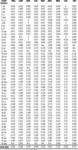
(7) 3.2) DNS Dataset: DNS (1995) provide estimates of education stocks based on mean school years of education per working person for working age population between the ages of 15 and 64 for 85 countries over 28 continuous years (196087). Theirs is an improvement over BL (1993, 1996) on several grounds. First, their calculation is based on enrolments nett of drop-out and retention rates at each grade and year.. Secondly, they made adjustments for depreciation of. education stock by incorporating the age-specific mortality rate for each enrollee in each grade in a year. Thirdly, as has been argued by the authors themselves, by dividing the primary, secondary and tertiary education stocks (in personyears) by the working population (in persons), this database captures the human-capital intensity of the work force. Unlike BL (1996), DNS do not have any proxy measure for quality of educational investment.. From the foregoing. discussion, it is evident that the DNS database scores over BL. We now discuss the methodology adopted for checking consistencies between each of these alternative definitions and the skilled labor payment share calculated from the GTAP database. The primary motivation is to find any correlation between human capital (proxied by average years of schooling and/or, enrolment, at different levels of education) and the GTAP data on the payment shares of skilled labor. For this purpose, we consider both BL (1996) and DNS (1995) data sets and see how these alternative measures of human capital stock are related to the skilled labor payment shares in the GTAP database. Thus, following DNS (1995), we consider mean school years of education per working age person as a potential index of human capital (MEDY_AC), expecting that the higher is MEDY_AC, the higher will be the skilled payment share. Similar consideration applies in the case of BL (1996) where average schooling years in the total population (TYR_BL) proxies human capital formation. We start with the construction of skilled labor payment share (SKL_AC) at the sectoral and aggregative levels according to the Version 4 of GTAP database. Sector-wide skilled payment share (SKL_ACi) for each traded GTAP sector ‘i’ is defined as the ‘share of skilled labor payment to total labor payment in that sector for any GTAP region r’. All these sectoral indexes are reported in Appendix. 4.

(8) Table A1.. The region-specific aggregative share SKL_ACr is the ratio of total. skilled labor payments to aggregate labor payments across all 50 sectors. Our next step is to match the GTAP regions with those covered in the BL (1996) and DNS (1995) databases for educational attainment and then to plot the scattergrams for the matched observations of the data sets. which data are available are considered.. All countries for. However, contingent upon which. regions have the necessary data, we include a subset of the GTAP regions in each regression. We exclude those regions (composite as well as single) which are not common in all these data sets.. Moreover, for some of the GTAP composite. regions not covered in either of the data sets for educational attainment, we have calculated simple averages of the data points related to schooling years of education for their component countries. This procedure assigns equal weights to each of the component countries, and hence does not reflect relative size differences of the constituent countries. Subsections below document our proposed consistency checks. 3.3) Reconciliation of GTAP Database and DNS(1995) Database Since GTAP uses average years of tertiary education in the work force as an index of educational attainment in the construction of the database 4, we consider mean years of tertiary education per working person as an indicator of human capital stock (MTRY_AC).. However, as mentioned before, because. MEDY_AC encapsulates mean years of total education at all levels of education, it is a suitable candidate index for human capital for the working age persons between age-group 15 and 64. Our choices of countries are governed by the data availability for each of MTRY_AC and MEDY_AC series. So far as the single regions are concerned, we exclude Vietnam (VNM), Taiwan (TWN), Hong Kong (HKG) and Former Soviet Union (FSU) as the data for them are missing in DNS (1995). Version 4 of the 4. In GTAP, a linear regression model relating skilled payment share to the country-wide per capita GDP (measured at 1987 prices) and the educational attainment has been fitted. It recognises that “the average years of tertiary education and the average years of secondary education for the whole work force can be used to represent the educational attainment”. However, the variable of secondary education is dropped on the ground that “after the regression, …[it] is not significant for the model.” (see pg. 18-3, Chapter 18, GTAP Version 4 Database). By adopting a broader definition as MEDY_AC, however, we, incorporate education at the tertiary as well as secondary and primary level in our proxy measure of human capital induced absorption capacity.. 5.

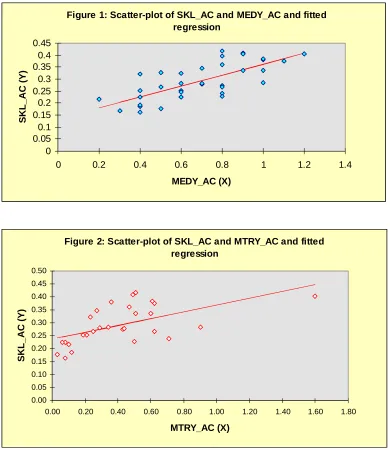
(9) GTAP database has 12 composite regions of which 5 are excluded on the same grounds as before and also due to our lack of information about their individual country coverage in the GTAP database. These five composite regions are Rest of South America (RSM), Central European Associates (CEA), Rest of Middle East (RME), Rest of Southern Africa (RSA), and the Rest of the world (ROW). For the remaining 7 composite GTAP regions, we have calculated simple averages of DNS data of MEDY_AC for 1987 for their component countries to derive the composite regions’ MEDY_AC. These 7 composite regions are Rest of Asia (RAS-includes Bangladesh, Pakistan, Myanmar), Central America and Caribbean (CAM-includes Jamaica and El Salvador), Rest of Andean Pact (RAP-includes Bolivia, Ecuador, Peru), Rest of European Union (REU-includes France, Greece, Ireland, Italy, Luxembourg, Netherlands, Portugal, Spain), EFT (Iceland, Norway, Switzerland), Rest of North Africa (RNF-includes Tunisia) and Rest of Sub-Saharan Africa (RSS-includes Senegal, Zimbabwe). We drop HKG, TWN, VNM from our sample of selected countries. Table A2 presents the list of all GTAP regions and the values of SKL_AC and MEDY_AC without exclusion of the regions/countries not covered in the DNS study. Table A3 reports their values for the matched country list. For MTRY_AC, the number of matched regions are reduced to 28 as DNS (1995) does not have data for them. The regions excluded are mostly composite regions viz., CAM, RAS, RAP, REU, EFT, RNF, RSS and single region SAF. These are reported in Table A4. All these tables are presented in the appendix. SKL_AC is now plotted against MEDY_AC and MTRY_AC across regions in two scatter diagrams in Figures 1 and 2, which also show fitted regression lines. However, we made adjustments to the DNS data for MEDY_AC. This is due to the fact that in our sample of observations the values of SKL_AC lie between 0.163 and 0.416 whereas the values for MEDY_AC vary from 2 to 12; for graphical presentation, we have scaled MEDY_AC by dividing all values by 10. USA is the outlier in both the scatter plots.. 6.

(10) SKL_AC (Y). Figure 1: Scatter-plot of SKL_AC and MEDY_AC and fitted regression 0.45 0.4 0.35 0.3 0.25 0.2 0.15 0.1 0.05 0 0. 0.2. 0.4. 0.6. 0.8. 1. 1.2. 1.4. MEDY_AC (X). Figure 2: Scatter-plot of SKL_AC and MTRY_AC and fitted regression 0.50 0.45. SKL_AC (Y). 0.40 0.35 0.30 0.25 0.20 0.15 0.10 0.05 0.00 0.00. 0.20. 0.40. 0.60. 0.80. 1.00. 1.20. 1.40. 1.60. 1.80. MTRY_AC (X). Both scatter plots show distinctive upward co-movements between SKL_AC and the relevant measure of human capital (MEDY_AC or MTRY_AC). Typically, our equation to be estimated is written as: SKL_ACr = A + b Xr + εr. (3.1). where Xr ∈ { MEDY_ACr, MTRY_ACr } and SKL_ACr is regressed on each Xr individually to estimate the intercept ‘A’ and the slope parameter ‘b’. ‘r’ ranges over a cross-section of countries/regions. The εr’s are assumed to be identically,. 7.

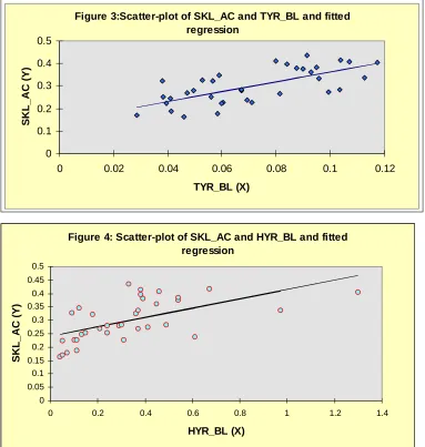
(11) 2. independently distributed with zero mean and constant variance (σ. ε. ).. The. estimation procedure is the OLS regression method. The fitted regression lines for each Xr are shown below. t-statistics are included in the parentheses below the estimated coefficients. 2 ^ SKL_AC = 0.1345 + 0.227 MEDY_AC r, R =0.53, F=38.43 r. (5.069). (3.1a). (6.20). and 2 ^ SKL_AC = 0.237 + 0.131 MTRY_AC r, R =0.33, F=12.93 r. (12.51). (3.1b). (3.60). Inspection of Figures 1 and 2 reveals that the extremely high level of MTRY_AC (but non-extreme value of SKL_AC) in USA is substantially responsible for the difference between the estimated slopes in the two regressions. 5 Using the t-statistics, we would reject the null hypothesis (that ‘b’ is zero) at the 1 per cent as well as the 5 percent level of significance in both cases. As expected, these significant t-statistics on the estimated slope parameter ‘b’ support the postulated relationship between SKL_AC and both the proxies of educational attainment level. The data used by the GTAP researchers (MTRY_AC) surprisingly does not fit the GTAP skill shares as well as the alternative (MEDY_AC). 3.4) Reconciliation of GTAP Database and BL (1996) Database In the case of the BL database, the number of matched observations is 35. Similar considerations to those applying to the DNS data set govern the selection of regions in conformity with GTAP database. The regions excluded are VNM, MAR, RAS, RME, RSM, REU, CEA, FSU, RSA and ROW.. We consider two. measures of educational attainment available in the BL (1996-7) data set viz., ‘average years of higher schooling in the total population’ (HYR_BL) and ‘average schooling years in the total population’ (TYR_BL) for the population aged 15 and over. TYR_BL includes average years of primary, secondary and higher schooling for the relevant age group in the total population. This has been motivated by our curiosity to check whether ‘total schooling years’ is better than ‘higher. 8.

(12) schooling years’ as a proxy for human capital.. All these figures are reported in. Table A5 of the appendix. Scattergrams of SKL_AC values plotted against TYR_BL and HYR_BL respectively are shown with the corresponding fitted regression lines in Figures 3 and 4.. As in the case of the DNS data set, we have normalised TYR_BL by. dividing all values by 10.. Figure 3:Scatter-plot of SKL_AC and TYR_BL and fitted regression. SKL_AC (Y). 0.5 0.4 0.3 0.2 0.1 0 0. 0.02. 0.04. 0.06. 0.08. 0.1. 0.12. TYR_BL (X). Figure 4: Scatter-plot of SKL_AC and HYR_BL and fitted regression 0.5. SKL_AC (Y). 0.45 0.4 0.35 0.3 0.25 0.2 0.15 0.1 0.05 0 0. 0.2. 0.4. 0.6. 0.8. 1. 1.2. 1.4. HYR_BL (X). The scatter plots show that SKL_AC has a positive correlation with both the BL-measures of human capital formation.. The correlation is stronger for. TYR_BL, though.. 5. Exclusion of USA from the sample of observations increases the value of the estimated 2 slope coefficient in (3.1b) to 0.169 whilst R = 0.30.. 9.

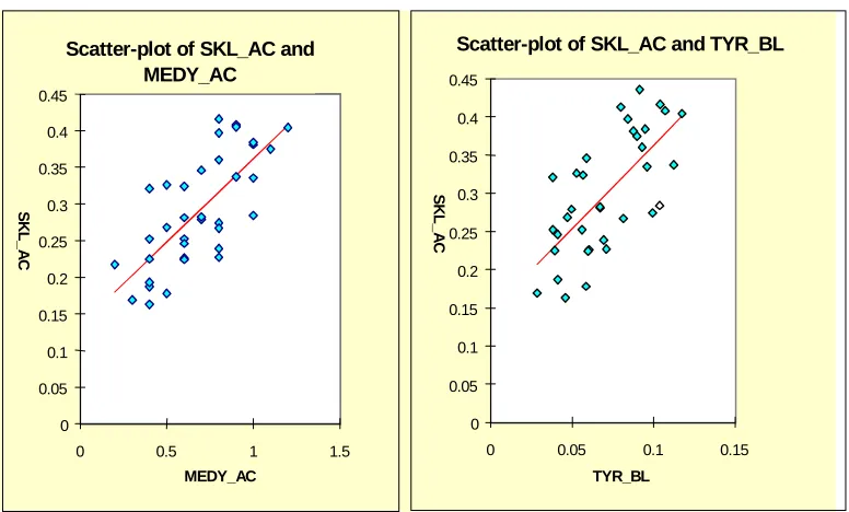
(13) As before, we fit a linear regression model linking SKL_AC with TYR_BL and HYR_BL. The equation we estimated is written below: SKL_ACr = A + b Xr + εr. (3.2). where Xr ∈ { TYR_BLr, HYR_BLr } and all other variables are defined as before. The fitted regression line for each Xr is given below. 2 ^ = 0.144 + 2.182 TYR_BL r, R = 0.48, F = 30.62 SKL_AC r. (4.871). (3.2a). (5.533). and 2 ^ SKL_AC = 0.241 + 0.173 HYR_BL r, R = 0.35, r. F = 17.44. (3.2b). (13.65) (4.18) 2. The higher value of R and the t-statistics on the slope coefficient in the case of (3.2a) suggest that mean years of total education (schooling) over all levels of education is a better measure of skill intensity of the workforce than the average schooling years at a specific level of education (such as tertiary or secondary). Comparison of the fitted regression lines for (3.1a) and (3.2a) as shown in Figure 5 demonstrates that MEDY_AC and TYR_BL exhibit almost exactly the same degree of compatibility with the SKL_AC data calculated from the GTAP database. Figure 5: Comparison between the regression lines Scatter-plot of SKL_AC and TYR_BL. Scatter-plot of SKL_AC and MEDY_AC. 0.45. 0.45 0.4. 0.4. 0.35. 0.35 SKL_AC. SKL_AC. 0.3 0.25. 0.3 0.25. 0.2. 0.2. 0.15. 0.15. 0.1. 0.1. 0.05. 0.05 0. 0 0. 0.5. 1. 0. 1.5. MEDY_AC. 0.05. 0.1 TYR_BL. 10. 0.15.

(14) Nevertheless, the regression involving the DNS data (MEDY_AC) fits the skilled share data slightly better than the BL data (TYR_BL). As seen above in Section 2b, the DNS (1995-96) data is also preferred on other grounds. Having specified an a priori relationship between various measures of human capital formation and skilled labor payment share and having checked the relationship statistically, it can be inferred (as expected) from the previous analysis that educational attainment explains quite significantly the GTAP shares of aggregate labor payments going to the skilled work force. This prompted us to investigate whether skilled labor embodying human capital and ‘raw’ or unskilled labor can be combined in a production nest which allows for substitutability between them. A ‘reasonable’ estimated value of the elasticity of substitution between them would validate our surmise in the sense that the existing GTAP data, including the partition of the wage bill into skilled and unskilled, is consistent with an empirically realistic degree of substitutability between the two classes of labor. The next section documents a formal theory to rationalize the procedures and the results of the skill disaggregation in GTAP.. 4. From Empirics to Theory 4.a) Production Nest In the GTAP production structure, the standard production technology tree is a nested production function where a CES-primary factor composite of Land (T), Labor (E) and Capital (K) combines with a CES intermediate composite of domestically sourced and foreign sourced intermediate inputs at the top level in a Leontief nest to produce final gross output (Y).. This gross production. function is separable into a value-added nest (nett output) and a nest of intermediate inputs. For incorporating human capital and relating it to skilled labor payment shares, we add a new nest to the production structure so that labor is now split into two components, raw labor (L u) and skilled labor (L s), so that total effective labor (E) is a constant elasticity of substitution (CES) combination of Ls and Lu.. The underlying assumption is that human capital. does not enter as an additional independent factor of production in the conventional way; rather, human capital proxied by educational attainment is. 11.

(15) embodied in the supply of skilled labor. Competition ensures that the payment to the labors with skill differentials are proportionate to their productivities. Such a production nesting is shown in Figure 6. Figure 6: A Production tree for GTAP incorporating human capital Final Output (Y). Intermediate Inputs Composite(M). Primary Factor Composite (Q). Land (T) Domestic Intermediate Input (Md). Foreign Composite Intermediate Input (Mf ). Imported Intermediates from Different Sources (Mf1 , Mf2 , Mf3 , ...). Effective Labor (E). Skilled labor (L s ) with embodied Human Capital. Capital (K). Raw or Unskilled Labor (L u). Thus, the production function for nett output is written as: Y = BH (K, T, E). (4.1). where ‘H’ is homogeneous of degree one (i.e., constant returns to scale) in the factor inputs and B is a technological coefficient. In intensity form, (4.1) is written as: y = B h (k, t). (4.2). where y = Y/E, k = K/E, and t = T/E. As we assume that ‘Ls’ and ‘Lu’ are combined in a Constant Elasticity of Substitution (CES) production nest to yield ‘E’, we write E. E=Γ[δ. u. −ρ. E. (Lu) + δ s (Ls). −ρ −1/ρ. ]. 12. (4.3).

(16) Note that σ =1/(1+ρ) is the elasticity of substitution between L s and Lu. (4.3) may be written: E. δ s (Ls). −ρ. = (E/Γ). −ρ. E. −δ. u. (Lu). −ρ. (4.4). E. δ j’ s are the distribution parameters which can be normalised to sum to unity (provided Γ is chosen appropriately). The shares of each factor computed from the quantity side are expressed as: E. −ρ. Sj = δ jXj /∑k δk Xk. −ρ. (4.5). where j is either of the categories of labor i.e., Ls or Lu. Equations (4.4) and (4.5) yield E. −ρ. Sj = δ jXj /(E/Γ). −ρ. (4.6). Therefore, −ρ E. Sj = Γ δ j (Xj/E). −ρ. (4.7). When Xj = Ls, we can write that Skilled labour payment share = [Constant] × [Distribution parameter] × −ρ. [Human Capital intensity] . Natural logarithmic transformation of (4.7) yields E. ln SLs = −ρ ln (Ls/E) + ln δ j − ρ ln Γ or, E. ln SLs = (ln δ j − ρ ln Γ) − ρ ln (Ls/E). (4.8). where SLs is SKL_AC in our notation for calculation of skilled labor payment share as described in Sections 2 and 3 above.. 4.b) Estimation Procedure Equation. (4.8). is. estimated. from. the. GTAP. regions/countries to find the estimated coefficient ρ. regression model fitted for estimating ρ is. 13. cross. section. of. Hence, the log-linear.

(17) ln SLs = Λ − ρ ln (Ls/E) + εI E. where Λ = (ln δ regression line.. j. (4.9). − ρ ln Γ) is a constant representing the intercept of the fitted By applying the OLS estimation procedure, we get the least-. squares estimate ^ ρ of ρ.. This is used to calculate the estimated value of the. σ. The elasticity of substitution between skilled labor (L s) and raw labor (Lu) i.e., ^ estimated standard error and approximate t-value of ^ σ are also derived6. This method has been followed for both the data sets viz., BL and DNS.. The. estimation results are discussed in the following section.. 5. Estimation Results As mentioned in Section 3, the educational attainment data for the selected GTAP composite regions are obtained by calculating the simple averages of the education data for the constituent countries. Here, for estimating σ, we present one set of results i.e., excluding those composite regions. However, values of ^ σ do not differ substantially if we include these composite regions from our sample of observations.7 The list of the sample regions included in the regressions are presented in the Tables A6 and A7 in the appendix.. 6. From the asymptotic distribution theory for large sample sizes (N→∞), we can say that for any differentiable scalar function ζ of a random variable Ψ, the asymptotic mean and variance-covariance matrix of ζ respectively are ζ (E (Ψ) ) and j′∑j, where E indicates asymptotic expectation, ∑ is the asymptotic variance-covariance matrix of Ψ, and j is matrix of derivatives of the elements of ζ with respect to those of ζ evaluated at Ψ = E(Ψ). In practice, we estimate E(Ψ) by Ψ, an unbiased estimate of E (Ψ), in order to evaluate the entities above. In the present application, ζ and Ψ are scalars. In fact, ζ ≡ σ, our estimated inter-skill substitution elasticity, while Ψ ≡ ^ ρ (our estimate of ρ). ^) = 1/(1+ρ ^) and j = ∂{1/(1+ρ ^)}/∂ρ ^ (evaluated at our estimate–ρ ^) = −1/(1+ρ ^)2 . Thus, ζ(ρ ^ Therefore, our estimated (asymptotic) standard error for our estimate ζ of σ is ≅ √ [(∂σ 2 2 ^ ^ ^ ^ ⁄∂ρ) Var(ρ) ]= [1/(1+ρ) ] × Standard error (ρ). See A. Goldberger, Econometric Theory (New York: Wiley, 1964), pp. 115-125 for detailed theoretical derivations which are beyond the scope of this paper.. 7. The regression equations incorporating the composite regions in the sample have R of ρ are 0.4799 0.50 (in case of DNS) and 0.47 (in case of BL). The estimated ^ (t-statistics=5.891) and 0.505 (t-statistics=5.433) for DNS and BL respectively. Estimated σûs are 0.6757 (approximate t-statistics=18.165) and 0.6644 (approximate tstatistics=16.19) for DNS and BL respectively. For MTRY_AC, we have the same sets of regions. Table A8 in the appendix reports these results.. 2. 14.

(18) The regression model fitted is the one specified in Equation (4.9). ^ ρ is the slope estimate resulting from the specific sample used in each regression. We use logarithmic transformation of MEDY_AC and MTRY_AC—both from the DNS data sets—as a proxy for [L s/E] in separate regressions. Also, natural logarithmic transformation of TYR_BL from BL (1996-97) has been used as a proxy for [L s/E]. Table 1 summarises the results from regressions using these alternative proxies for educational attainment. From the results, we observe that in case of TYR_BL and MEDY_AC, the elasticity of substitution between skilled and unskilled labor [i.e., σ ] is relatively us. well. determined,. with. point. estimates. in. the. range. of. 0.67-0.70.. t-statistics for tests of significant difference both from zero and from unity exceed 6.. The latter result indicates significant difference from a Cobb-Douglas. specification for the aggregator of the two types of labor. 8 The estimated value σûs of σus in the case where MTRY_AC is the proxy for human capital intensity yields the highest of the results obtained (0.83).. The. ranking of σûs in terms of their estimated magnitudes based on alternative measures of educational attainment is. σûs(MTRY_AC) > σûs(MEDY_AC) > σûs(TYR_BL). Empirical evidence of the elasticity of substitution between different skill categories in the Australian economy9 suggests the following point estimates (for the Australian economy), for the value of ‘σ’: between skilled white collar and unskilled white collar, 0.63; between unskilled blue collar and skilled white collar, 0.24; between unskilled white collar and skilled blue collar, 0.75. The first and last of these numbers suggest that the values of σûs found above are reasonable.. 8. The calculation involved is: new t-statistics = ( σûs− 1)/(estimated standard error of σûs).. 9. Higgs, Peter J., Dean Parham, and Brian Parmenter (1981) “Occupational Wage Relativities and labour-labour substitution in the Australian Economy: Applications of the ORANI model. IMPACT Project, Preliminary Working Paper No. OP-30, Melbourne, August 1981. They reported ‘implied’ CRESH elasticity of substitution between occupations in ORANI simulations.. 15.

(19) Table 1:. Elasticity of substitution regressions excluding GTAP composite regions*. Dependent Variable: Skilled labour’s share in total labor payment, (SKL_AC) Independent Variables. Mean years of edu- Mean years of tertiary Mean years of cation per working education per working schooling in total person (MEDY_AC) person(MTRY_AC) population (TYR_BL). Data Set. DNS (1995-96). Observations. DNS (1995-96). BL (1995-96). 29. 28. 30. R. 0.42. 0.53. 0.39. F-value. 19.18. 29.70. 18.14. 0.4156. 0.2088. 0.4943. 4.3793. 5.4499. 4.2596. 0.7064. 0.8272. 0.6692. 14.9163. 31.544. 12.8769. -6.1996. -6.5895. -6.3653. 2. ρ Estimated ^ ρ t-statistics for ^. (a). Estimated σ^. us. approximate t-statistics for σ^. (a). us. approximate t-statistics for σ^. (b). us. * All variables are in natural logarithms. (a) Test for significant difference from zero. (b) Test for significant difference from 1.. 6. Summary We have been concerned here to identify educational data that can be used as a proxy for human capital endowment. The above analysis reveals that the available alternative educational attainment data sets all conform with the share of aggregate labor payments accruing to the skilled labor categories incorporated in the Version 4 of GTAP database.. This comes as no surprise,. since the GTAP labor split is based on one of these educational data sources. However, there is room for disagreement on some of the details. Amongst the alternative data sources, DNS (1995) data scores over BL (1996) on some desirable grounds. The derivation by Liu et al. (1998) of the shares of skilled and unskilled labor in the work force of the 45 GTAP regions from data on educational. 16.

(20) attainment follows an ad hoc regression approach. In this paper the GTAP data on such shares have been taken as given, although it might have been preferable if the shares had been derived within a production-theoretic framework. Given the shares, we offer an ex post rationalization of them within such a framework, thereby deriving estimates of the elasticity of substitution between skilled and unskilled labor. This relies on the inter-regional covariation in the GTAP shares and in measures of educational attainment. The resulting point estimates are in the range 0.67 (±0.05) to 0.83 (±0.03), depending on the educational data used. These point estimates differ significantly from zero and from unity at a high level of significance.. 17.

(21) REFERENCES. Barro, Robert J. and Jong Wha Lee (1996) (BL), “International Measures of Schooling Years and Schooling Quality”, American Economic Review, Papers and Proceedings, Vol. 86, No. 2, pp. 218-23. Barro, Robert J. and Jong Wha Lee (1993), “International comparisons of Educational Attainment”, Journal of Monetary Economics, Vol. 32, No. 3, pp. 363-94. Liu, Jing, Nico Van Leeuwen, Tri Thanh Vo, Rod Tyres and Thomas Hertel (1998), “Disaggregating Labor Payments by Skill Level”, Ch. 18, Version 4 of GTAP database, Centre for Global Trade Analysis, Purdue University, USA. Nehru, Vikram, Eric Swanson and Ashutosh Dubey (1995) (DNS), “A New Database on Human Capital Stock. in Developing and. Countries: Sources, Methodology, and Results”, Journal of. Industrial. Development. Economics, Vol. 46, pp. 379-401. Nehru, Vikram, and Ashok Dhareshwar (1993), “ A New Database on Physical Capital Stock: Sources, Methodology and Results”, Rivista de Analisis Economico, Vol. 8, No. 1, pp. 37-59. World Education Report (1993), UNESCO.. 18.

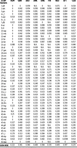
(22) Table A1: Skilled labor payment shares in GTAP sectors and regions GTAP Regions GTAP Sectors. AUS. NZL. JPN. KOR. IDN. MYS. PHL. SGP. THA. 1 pdr 2 wht 3 gro 4 v_f 5 osd 6 c_b 7 pfb 8 ocr 9 ctl 10 oap 11 rmk 12 wol 13 for 14 fsh 15 col 16 oil 17 gas 18 omn 19 cmt 20 omt 21 vol 22 mil 23 pcr 24 sgr 25 ofd 26 b_t 27 tex 28 wap 29 lea 30 lum 31 ppp 32 p_c 33 crp 34 nmm 35 i_s 36 nfm 37 fmp 38 mvh 39 otn 40 ele 41 ome 42 omf 43 ely 44 gdt 45 wtr 46 cns 47 t_t 48 osp 49 osg 50 dwe. 0.067 0.052 0.049 0.052 0.054 0.052 0.052 0.051 0.052 0.051 0.053 0.052 0.052 0.050 0.192 0.398 0.398 0.239 0.253 0.252 0.256 0.253 0.241 0.254 0.253 0.254 0.273 0.274 0.274 0.194 0.295 0.455 0.397 0.248 0.289 0.289 0.258 0.245 0.245 0.390 0.390 0.264 0.365 0.365 0.365 0.254 0.281 0.483 0.654 0.000. N.A. 0.028 0.026 0.034 0.000 N.A. 0.000 0.048 0.034 0.035 0.033 0.034 0.029 0.050 0.133 0.300 0.263 0.211 0.192 0.200 0.231 0.185 0.250 0.230 0.230 0.216 0.179 0.167 0.173 0.178 0.256 0.265 0.289 0.209 0.202 0.213 0.218 0.257 0.258 0.306 0.305 0.208 0.342 0.333 0.350 0.214 0.229 0.456 0.566 N.A.. 0.015 0.015 0.014 0.015 0.018 0.015 0.000 0.015 0.015 0.015 0.015 0.000 0.015 0.015 0.412 0.429 0.409 0.410 0.311 0.310 0.308 0.310 0.311 0.310 0.310 0.390 0.272 0.153 0.153 0.351 0.415 0.376 0.370 0.378 0.368 0.378 0.361 0.400 0.400 0.382 0.382 0.345 0.417 0.417 0.417 0.421 0.387 0.407 0.365 0.000. 0.005 0.000 0.005 0.005 0.000 N.A. 0.000 0.004 0.007 0.005 0.005 0.000 0.004 0.005 0.143 N.A. N.A. 0.152 0.246 0.243 0.273 0.202 0.268 0.222 0.254 0.213 0.163 0.162 0.124 0.174 0.296 0.201 0.281 0.210 0.206 0.224 0.221 0.231 0.231 0.269 0.269 0.185 0.152 0.152 0.152 0.167 0.206 0.352 0.473 N.A.. 0.000 N.A. 0.001 0.001 0.002 0.000 0.001 0.000 0.002 0.000 0.000 N.A. 0.001 0.000 0.261 0.261 0.120 0.261 0.117 0.113 0.115 0.200 0.115 0.116 0.115 0.116 0.155 0.123 0.154 0.117 0.239 0.239 0.239 0.239 0.239 0.240 0.239 0.239 0.240 0.239 0.239 0.065 0.493 0.492 0.490 0.154 0.084 0.320 0.553 0.000. 0.013 N.A. 0.000 0.014 0.012 0.000 0.000 0.013 0.000 0.013 0.017 N.A. 0.012 0.015 N.A. 0.184 0.149 0.140 0.000 0.170 0.190 0.154 0.188 N.A. 0.188 0.142 0.153 0.131 0.000 0.132 0.181 0.212 0.193 0.164 0.168 0.179 0.168 0.174 0.176 0.197 0.197 0.135 0.354 0.355 0.351 0.174 0.204 0.410 0.593 0.000. 0.019 0.000 0.018 0.019 0.000 0.019 0.029 0.019 0.016 0.019 0.000 N.A. 0.019 0.019 0.000 N.A. 0.200 0.113 0.079 0.073 0.167 0.051 0.122 0.167 0.167 0.109 0.099 0.129 0.104 0.086 0.152 0.000 0.210 0.118 0.095 0.114 0.133 0.182 0.167 0.231 0.230 0.092 0.248 0.253 0.245 0.101 0.091 0.514 0.633 0.000. N.A. N.A. N.A. 0.033 0 0 0 0.040 0 0.038 0 N.A. N.A. 0 N.A. N.A N.A. 0 0 0.269 0.269 0.278 N.A. 0.250 0.264 0.271 0.224 0.180 0.212 0.234 0.314 0.397 0.324 0.280 0.274 0.280 0.262 0.290 0.293 0.332 0.332 0.266 0.400 0.411 0.407 0.286 0.323 0.402 0.525 N.A.. 0.001 N.A. 0.000 0.000 0.000 0.002 0.000 0.000 0.000 0.000 0.000 0.000 0.002 0.000 0.086 0.172 0.142 0.132 0.146 0.145 0.182 0.133 0.160 0.182 0.182 0.129 0.135 0.129 0.133 0.116 0.168 0.169 0.193 0.147 0.140 0.171 0.153 0.171 0.170 0.200 0.201 0.118 0.322 0.333 0.321 0.150 0.169 0.438 0.606 0.000. REGION-WIDE 0.416. 0.337. 0.375. 0.274. 0.163. 0.226. 0.239. 0.346. 0.252. Source: Calculated from Version 4 of GTAP Database. 19.

(23) Table A1(continued): Skilled labor payment shares in GTAP sectors and regions GTAP Regions GTAP Sectors. VNM. CHN. HKG. TWN. IND. LKA. RAS. CAN. USA. 1 pdr 2 wht 3 gro 4 v_f 5 osd 6 c_b 7 pfb 8 ocr 9 ctl 10 oap 11 rmk 12 wol 13 for 14 fsh 15 col 16 oil 17 gas 18 omn 19 cmt 20 omt 21 vol 22 mil 23 pcr 24 sgr 25 ofd 26 b_t 27 tex 28 wap 29 lea 30 lum 31 ppp 32 p_c 33 crp 34 nmm 35 i_s 36 nfm 37 fmp 38 mvh 39 otn 40 ele 41 ome 42 omf 43 ely 44 gdt 45 wtr 46 cns 47 t_t 48 osp 49 osg 50 dwe. 0.007 N.A. 0.000 0.008 0.000 0.008 0.000 0.007 0.000 0.008 0.000 N.A. 0.012 0.000 0.111 0.155 0.095 0.118 0.000 0.158 0.200 0.000 0.167 0.125 0.176 0.120 0.143 0.122 0.136 0.110 0.167 N.A. 0.171 0.146 0.167 0.000 0.250 0.167 0.167 0.161 0.165 0.115 0.350 N.A. 0.000 0.153 0.183 0.409 0.606 0.000. 0.008 0.008 0.008 0.008 0.008 0.007 0.008 0.008 0.008 0.008 0.008 0.007 0.008 0.008 0.107 0.155 0.113 0.124 0.165 0.162 0.178 0.146 0.162 0.177 0.177 0.120 0.140 0.121 0.136 0.113 0.155 0.175 0.167 0.147 0.151 0.159 0.150 0.151 0.151 0.170 0.170 0.109 0.345 0.344 0.344 0.154 0.185 0.408 0.605 0.000. N.A. N.A. N.A. 0.059 N.A. N.A. 0 0.0588 0.0597 0.0586 N.A. N.A. N.A. 0.091 N.A. 0 N.A. 0.217 0.333 0.333 0.333 0.330 N.A. N.A. 0.327 0.328 0.304 0.260 0.399 0.265 0.419 N.A. 0.393 0.357 0.303 0.286 0.315 0.451 0.452 0.452 0.451 0.353 0.474 0.47 0.471 0.270 0.428 0.451 0.682 0. 0.030 0.000 0.030 0.030 0.031 0.029 0.000 0.029 0.030 0.029 0.038 0.000 0.025 0.030 0.091 0.200 0.245 0.218 0.246 0.245 0.345 0.208 0.233 0.346 0.343 0.187 0.242 0.144 0.179 0.214 0.199 0.204 0.262 0.212 0.172 0.230 0.221 0.268 0.268 0.322 0.322 0.226 0.391 0.391 0.392 0.216 0.335 0.369 0.775 0.000. 0.001 0.001 0.001 0.001 0.001 0.001 0.001 0.001 0.001 0.001 0.001 0.000 0.001 0.000 0.096 0.156 0.114 0.122 0.125 0.000 0.175 0.142 0.161 0.175 0.175 0.118 0.134 0.122 0.130 0.109 0.153 0.171 0.171 0.142 0.141 0.151 0.149 0.154 0.154 0.175 0.176 0.106 0.332 0.333 0.332 0.146 0.171 0.422 0.609 0.000. 0.006 N.A. N.A. 0.007 0.000 0.000 0.000 0.009 0.000 0.000 0.000 N.A. 0.000 0.014 0.000 N.A. N.A. 0.122 0.000 N.A. 0.000 0.125 0.200 N.A. 0.179 0.143 0.141 0.122 0.167 0.111 0.143 0.000 0.169 0.140 0.200 0.000 0.143 0.000 0.200 0.200 0.154 0.000 0.343 0.333 0.357 0.153 0.181 0.414 0.606 N.A.. 0.009 0.009 0.010 0.009 0.009 0.009 0.010 0.009 0.008 0.009 0.009 0.000 0.010 0.009 0.143 0.147 0.115 0.122 N.A. N.A. 0.176 0.148 0.000 0.176 0.175 0.114 0.133 0.123 0.130 0.107 0.153 0.000 0.172 0.142 0.141 0.167 0.167 0.151 0.155 0.200 0.179 0.105 0.330 0.318 0.333 0.145 0.170 0.424 0.610 0.000. N.A. 0.078 0.078 0.079 0.078 0.083 N.A. 0.075 0.079 0.078 0.077 N.A. 0.078 0.078 0.269 0.268 0.268 0.268 0.180 0.180 0.181 0.180 N.A. 0.200 0.180 0.182 0.119 0.161 0.145 0.151 0.300 0.271 0.352 0.190 0.165 0.165 0.208 0.302 0.302 0.370 0.370 0.207 0.257 0.257 0.257 0.193 0.195 0.381 0.641 0.000. 0.071 0.071 0.071 0.071 0.071 0.071 0.071 0.071 0.071 0.071 0.071 N.A. 0.071 0.071 0.141 0.431 0.431 0.283 0.141 0.141 0.271 0.141 0.239 0.271 0.271 0.324 0.178 0.216 0.200 0.226 0.355 0.356 0.439 0.252 0.206 0.244 0.278 0.387 0.387 0.478 0.478 0.285 0.332 0.332 0.332 0.251 0.207 0.628 0.494 0.000. REGION-WIDE 0.177. 0.178. 0.436. 0.413. 0.187. 0.224. 0.193. 0.284. 0.404. Source: Calculated from Version 4 of GTAP Database. 20.

(24) Table A1(continued): Skilled labor payment shares in GTAP sectors and regions GTAP Regions GTAP Sectors. MEX. CAM. VEN. COL. RAP. ARG. BRA. CHL. URY. 0.014 0.017 0.017 0.017 0.024 0.017 0.019 0.018 0.017 0.017 0.017 0.000 0.017 0.019 0.091 0.198 0.167 0.148 0.153 0.153 0.185 0.143 0.000 0.194 0.190 0.146 0.142 0.136 0.140 0.127 0.183 0.189 0.211 0.159 0.152 0.168 0.166 0.187 0.188 0.221 0.221 0.133 0.326 0.324 0.326 0.161 0.179 0.443 0.599 N.A. 0.281 REGION-WIDE. 0.013 0.000 0.014 0.013 0.012 0.013 0.014 0.013 0.013 0.014 0.017 N.A. 0.014 0.011 0.088 0.176 0.134 0.131 0.149 0.136 0.175 0.140 0.162 0.179 0.180 0.128 0.134 0.128 0.137 0.117 0.164 0.168 0.188 0.147 0.142 0.167 0.155 0.167 0.165 0.195 0.195 0.115 0.325 0.325 0.326 0.149 0.170 0.434 0.607 0.000 0.246. 0.000 0.021 0.018 0.019 0.026 0 0 0.020 0.019 0.022 0.017 0 0 0.019 0.074 0.195 N.A. 0.138 0.125 0.167 0.184 0.119 N.A. 0.179 0.183 0.135 0.129 0.136 0.126 0.112 0.174 0.250 0.213 0.144 0.129 0.152 0.159 0.186 0.189 0.222 0.228 0.143 0.298 0.298 0.295 0.140 0.148 0.470 0.611 N.A. 0.279. 0.010 0.013 0.012 0.014 0.012 0.011 0.014 0.013 0.013 0.013 0.011 0.011 0.017 0.000 0.073 0.173 0.120 0.123 0.131 0.143 0.176 0.127 0.149 0.182 0.179 0.125 0.131 0.128 0.127 0.108 0.161 0.159 0.189 0.142 0.135 0.154 0.151 0.169 0.173 0.200 0.197 0.115 0.316 0.314 0.318 0.143 0.160 0.444 0.610 N.A. 0.268. 0.017 0.017 0.016 0.016 0.013 0.017 0.017 0.016 0.016 0.016 0.014 0.030 0.000 0.020 N.A. 0.178 0.134 0.121 0.100 0.118 0.167 0.095 0.160 0.176 0.174 0.117 0.116 0.132 0.113 0.098 0.155 0.134 0.199 0.133 0.117 0.141 0.148 0.176 0.172 0.213 0.214 0.104 0.288 0.276 0.294 0.125 0.131 0.474 0.620 N.A. 0.324. 0.032 0.027 0.027 0.027 0.027 0.028 0.026 0.028 0.027 0.027 0.027 0.026 0.026 0.027 0.000 0.238 N.A. 0.168 0.139 0.137 0.201 0.129 0.178 0.199 0.201 0.168 0.141 0.149 0.141 0.136 0.208 0.192 0.253 0.166 0.148 0.173 0.181 0.221 0.221 0.270 0.270 0.152 0.301 0.301 0.301 0.163 0.167 0.482 0.667 N.A. 0.267. 0.034 0.035 0.034 0.034 0.034 0.034 0.032 0.034 0.034 0.034 0.034 N.A. 0.034 0.032 0.000 0.186 0.167 0.139 0.141 0.141 0.140 0.141 0.141 0.141 0.141 0.141 0.141 0.141 0.141 0.141 0.141 0.141 0.141 0.141 0.141 0.141 0.141 0.141 0.141 0.141 0.141 0.141 0.239 0.239 0.239 0.176 0.159 0.529 0.529 0.000 0.321. 0 0.017 0.022 0.017 0 0.020 0 0.013 0.015 0.017 0.014 0 0.015 0.02 0.077 0.200 0.200 0.14 0.14 0.140 0.333 0.137 0.000 0.19 0.19 0.14 0.14 0.13 0.13 0.12 0.18 0.17 0.21 0.15 0.14 0.16 0.16 0.18 0.18 0.22 0.22 0.14 0.32 0.32 0.32 0.15 0.17 0.45 0.60 0 0.282. 0.021 0.015 0.026 0.021 0.000 0.000 0.000 0.000 0.020 0.018 0.020 0.018 0.000 0.000 N.A. N.A. N.A. 0.125 0.120 0.000 0.200 0.108 0.182 0.200 0.184 0.143 0.136 0.135 0.129 0.125 0.185 0.250 0.221 0.144 0.143 0.250 0.164 0.184 0.200 0.243 0.231 0.133 0.300 0.333 0.296 0.145 0.150 0.474 0.609 0.000 0.227. 1 pdr 2 wht 3 gro 4 v_f 5 osd 6 c_b 7 pfb 8 ocr 9 ctl 10 oap 11 rmk 12 wol 13 for 14 fsh 15 col 16 oil 17 gas 18 omn 19 cmt 20 omt 21 vol 22 mil 23 pcr 24 sgr 25 ofd 26 b_t 27 tex 28 wap 29 lea 30 lum 31 ppp 32 p_c 33 crp 34 nmm 35 i_s 36 nfm 37 fmp 38 mvh 39 otn 40 ele 41 ome 42 omf 43 ely 44 gdt 45 wtr 46 cns 47 t_t 48 osp 49 osg 50 dwe. Source: Calculated from Version 4 of GTAP Database. 21.

(25) Table A1(continued): Skilled labor payment shares in GTAP sectors and regions GTAP Regions GTAP Sectors. RSM. GBR. DEU. DNK. SWE. FIN. REU. EFT. CEA. 0 0 0 0 0.014 0 0.015 0 0 0 0 0 0 0 0.088 0 N.A. 0.111 0.167 0 0 0.143 0 0.167 0.179 0.143 0.167 0.143 0 0.107 0.143 0.164 0.189 0.143 0 0 0.125 0 N.A. 0.25 0 0 0.327 0.316 0.333 0.150 0.170 0.432 0.610 0 0.222 REGION-WIDE. 0 0.042 0.043 0.042 0.042 0.041 0.063 0.042 0.042 0.042 0.042 0.040 0.043 0.038 0.256 0.341 0.338 0.267 0.265 0.265 0.266 0.261 N.A. 0.265 0.265 0.276 0.222 0.184 0.208 0.232 0.317 0.391 0.334 0.266 0.268 0.267 0.264 0.300 0.300 0.344 0.344 0.266 0.400 0.400 0.400 0.281 0.313 0.418 0.527 0 0.381. 0.059 0.054 0.054 0.054 0.055 0.054 0.053 0.054 0.054 0.054 0.054 0.056 0.054 0.054 0.313 0.411 0.420 0.319 0.305 0.305 0.297 0.302 0.308 0.297 0.297 0.332 0.252 0.207 0.234 0.276 0.376 0.471 0.394 0.310 0.312 0.307 0.305 0.353 0.353 0.407 0.407 0.323 0.423 0.423 0.423 0.329 0.361 0.419 0.498 0.000 0.360. N.A. 0.058 0.061 0.060 0.053 0.065 0.000 0.060 0.060 0.059 0.059 0.000 0.056 0.058 N.A. 0.438 0.458 0.348 0.329 0.327 0.314 0.325 N.A. 0.310 0.312 0.359 0.268 0.217 0.248 0.297 0.404 0.512 0.419 0.331 0.333 0.333 0.325 0.376 0.376 0.433 0.433 0.351 0.438 0.437 0.438 0.353 0.388 0.414 0.483 0 0.408. 0 0.066 0.061 0.063 0.063 0.064 0 0.066 0.063 0.063 0.063 N.A. 0.063 0.067 N.A. N.A. N.A. 0.352 0.322 0.323 0.317 0.321 N.A. 0.319 0.316 0.367 0.268 0.221 0.247 0.301 0.413 0.515 0.435 0.334 0.335 0.329 0.331 0.389 0.389 0.451 0.451 0.358 0.429 0.438 0.430 0.355 0.384 0.428 0.482 0 0.384. N.A. 0.056 0.049 0.052 0.048 0.041 N.A. 0.050 0.05 0.049 0.050 0 0.05 0.083 N.A. N.A. N.A. 0.289 0.258 0.260 0.273 0.256 N.A. 0.271 0.277 0.298 0.224 0.196 0.212 0.244 0.343 0.405 0.372 0.276 0.271 0.275 0.279 0.331 0.331 0.388 0.388 0.286 0.385 N.A. 0.385 0.289 0.310 0.446 0.521 N.A. 0.335. 0.071 0.068 0.068 0.068 0.068 0.068 0.067 0.068 0.068 0.068 0.068 0.071 0.068 0.068 0.295 0.664 0.665 0.323 0.263 0.263 0.239 0.248 0.280 0.239 0.239 0.269 0.211 0.178 0.195 0.194 0.301 0.548 0.370 0.250 0.269 0.248 0.248 0.283 0.283 0.380 0.380 0.237 0.574 0.574 0.574 0.242 0.270 0.536 0.563 0.000 0.405. 0 0.067 0.064 0.065 0.064 0.068 0.063 0.065 0.065 0.065 0.065 0 0.064 0.065 0.397 0.472 0.5 0.379 0.37 0.370 0.334 0.369 0.346 0.333 0.334 0.396 0.295 0.229 0.269 0.330 0.441 0.579 0.447 0.365 0.376 0.359 0.353 0.404 0.404 0.459 0.459 0.390 0.470 0.469 0.470 0.393 0.437 0.393 0.4599 0 0.397. 0.016 0.018 0.017 0.017 0.016 0.016 0.018 0.016 0.017 0.017 0.017 0.019 0.018 0.017 0.066 0.189 0.149 0.131 0.119 0.119 0.182 0.109 0.149 0.178 0.179 0.127 0.123 0.132 0.124 0.107 0.166 0.144 0.205 0.138 0.123 0.147 0.152 0.179 0.179 0.218 0.218 0.112 0.295 0.295 0.295 0.134 0.142 0.470 0.614 0.000 0.225. 1 pdr 2 wht 3 gro 4 v_f 5 osd 6 c_b 7 pfb 8 ocr 9 ctl 10 oap 11 rmk 12 wol 13 for 14 fsh 15 col 16 oil 17 gas 18 omn 19 cmt 20 omt 21 vol 22 mil 23 pcr 24 sgr 25 ofd 26 b_t 27 tex 28 wap 29 lea 30 lum 31 ppp 32 p_c 33 crp 34 nmm 35 i_s 36 nfm 37 fmp 38 mvh 39 otn 40 ele 41 ome 42 omf 43 ely 44 gdt 45 wtr 46 cns 47 t_t 48 osp 49 osg 50 dwe. Source: Calculated from Version 4 of GTAP Database. 22.

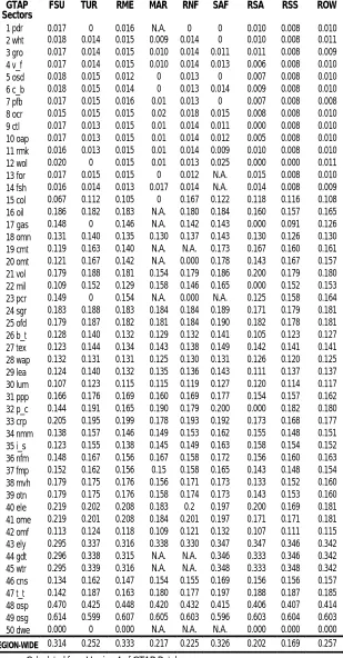
(26) Table A1(continued): Skilled labor payment shares in GTAP sectors and regions GTAP Regions GTAP Sectors. FSU. TUR. RME. MAR. RNF. SAF. RSA. RSS. ROW. 0.017 0.018 0.017 0.017 0.018 0.018 0.017 0.015 0.017 0.017 0.016 0.020 0.017 0.016 0.067 0.186 0.148 0.131 0.119 0.121 0.179 0.109 0.149 0.183 0.179 0.128 0.123 0.132 0.124 0.107 0.166 0.144 0.205 0.138 0.123 0.148 0.152 0.179 0.179 0.219 0.219 0.113 0.295 0.296 0.295 0.134 0.142 0.470 0.614 0.000 0.314 REGION-WIDE. 0 0.014 0.014 0.014 0.015 0.015 0.015 0.015 0.013 0.013 0.013 0 0.015 0.014 0.112 0.182 0 0.140 0.163 0.167 0.188 0.152 0 0.188 0.187 0.140 0.144 0.131 0.140 0.123 0.176 0.191 0.195 0.157 0.155 0.167 0.162 0.175 0.175 0.202 0.201 0.124 0.337 0.338 0.339 0.162 0.187 0.425 0.599 0 0.252. 0.016 0.015 0.015 0.015 0.012 0.014 0.016 0.015 0.015 0.015 0.015 0.015 0.015 0.013 0.105 0.183 0.146 0.135 0.140 0.142 0.181 0.129 0.154 0.183 0.182 0.132 0.134 0.131 0.132 0.115 0.169 0.165 0.199 0.146 0.138 0.156 0.156 0.176 0.176 0.208 0.208 0.118 0.316 0.315 0.316 0.147 0.163 0.448 0.607 0.000 0.333. N.A. 0.009 0.010 0.010 0 0 0.01 0.02 0.01 0.01 0.01 0.01 0 0.017 0 N.A. N.A. 0.130 N.A. N.A. 0.154 0.158 N.A. 0.184 0.181 0.129 0.143 0.125 0.135 0.115 0.160 0.190 0.178 0.149 0.145 0.167 0.15 0.156 0.158 0.183 0.184 0.109 0.338 N.A. N.A. 0.154 0.180 0.420 0.605 N.A. 0.217. 0 0.014 0.014 0.014 0.013 0.013 0.013 0.018 0.014 0.014 0.014 0.013 0.012 0.014 0.167 0.180 0.142 0.137 N.A. 0.000 0.179 0.146 0.000 0.184 0.184 0.132 0.138 0.130 0.136 0.119 0.169 0.179 0.193 0.153 0.149 0.158 0.158 0.171 0.174 0.2 0.201 0.121 0.330 N.A. N.A. 0.155 0.177 0.432 0.603 N.A. 0.225. 0 0 0.011 0.013 0 0.014 0 0.015 0.011 0.012 0.009 0.025 N.A. N.A. 0.122 0.184 0.143 0.143 0.173 0.178 0.186 0.165 N.A. 0.189 0.190 0.141 0.149 0.131 0.143 0.127 0.177 0.200 0.192 0.162 0.163 0.172 0.165 0.173 0.173 0.197 0.197 0.132 0.347 0.346 0.348 0.169 0.197 0.415 0.596 N.A. 0.326. 0.010 0.010 0.011 0.006 0.007 0.009 0.007 0.008 0.000 0.005 0.010 0.000 0.015 0.014 0.118 0.160 0.000 0.130 0.167 0.143 0.200 0.000 0.125 0.171 0.182 0.105 0.142 0.126 0.111 0.120 0.154 0.000 0.173 0.155 0.158 0.156 0.143 0.133 0.143 0.200 0.171 0.107 0.347 0.333 0.333 0.156 0.188 0.406 0.603 0.000 0.202. 0.008 0.008 0.008 0.008 0.008 0.008 0.008 0.008 0.008 0.008 0.008 0.000 0.008 0.008 0.116 0.157 0.091 0.126 0.160 0.167 0.179 0.152 0.158 0.179 0.178 0.123 0.141 0.120 0.137 0.114 0.157 0.182 0.168 0.148 0.154 0.160 0.148 0.152 0.153 0.169 0.171 0.111 0.346 0.346 0.348 0.156 0.187 0.407 0.604 0.000 0.169. 0.010 0.011 0.009 0.010 0.010 0.010 0.008 0.010 0.010 0.010 0.010 0.011 0.010 0.009 0.108 0.165 0.126 0.130 0.161 0.157 0.180 0.153 0.164 0.181 0.181 0.127 0.141 0.125 0.137 0.117 0.162 0.180 0.177 0.151 0.152 0.163 0.154 0.160 0.160 0.181 0.181 0.115 0.342 0.342 0.342 0.157 0.185 0.414 0.603 0.000 0.257. 1 pdr 2 wht 3 gro 4 v_f 5 osd 6 c_b 7 pfb 8 ocr 9 ctl 10 oap 11 rmk 12 wol 13 for 14 fsh 15 col 16 oil 17 gas 18 omn 19 cmt 20 omt 21 vol 22 mil 23 pcr 24 sgr 25 ofd 26 b_t 27 tex 28 wap 29 lea 30 lum 31 ppp 32 p_c 33 crp 34 nmm 35 i_s 36 nfm 37 fmp 38 mvh 39 otn 40 ele 41 ome 42 omf 43 ely 44 gdt 45 wtr 46 cns 47 t_t 48 osp 49 osg 50 dwe. Source: Calculated from Version 4 of GTAP Database. 23.

(27) Table A2: Mean years of education per working person and skilled labor payment shares for All GTAP Regions GTAP Skill Payment Share Education Years Regions (SKL_AC) (MEDY_AC) AUS NZL JPN KOR IDN MYS PHL SGP THA VNM CHN HKG TWN IND LKA RAS CAN USA MEX CAM VEN COL RAP ARG BRA CHL URY RSM GBR DEU DNK SWE FIN REU EFT CEA FSU TUR RME MAR RNF SAF RSA RSS ROW. 0.416 0.337 0.375 0.274 0.163 0.226 0.239 0.346 0.252 0.177 0.178 0.436 0.413 0.187 0.224 0.193 0.284 0.404 0.281 0.246 0.279 0.268 0.324 0.267 0.321 0.282 0.227 0.222 0.381 0.36 0.408 0.384 0.335 0.405 0.397 0.225 0.314 0.252 0.333 0.217 0.225 0.326 0.202 0.169 0.257. 8 9 11 8 4 6 8 7 6 N.A. 5 N.A N.A 4 6 4 10 12 6 6 7 5 6 8 4 7 8 N.A 10 8 9 10 10 9 8 N.A. N.A. 4 N.A. 2 4 5 N.A. 3 N.A.. Source: For MEDY_AC, DNS (1995), World Bank Dataset; for SKL_AC, Table A1.. 24.

(28) Table A3: Skilled labor payment shares and mean school years of education for selected GTAP regions GTAP Regions. AUS NZL JPN KOR IDN MYS PHL SGP THA CHN IND LKA RAS CAN USA MEX CAM VEN COL RAP ARG BRA CHL URY GBR DEU DNK SWE FIN REU EFT TUR MAR RNF SAF RSS. Skill Payment Share. School Years of Education. (SKL_AC). Scaled School Years of Education (MEDY_AC). 0.416 0.337 0.375 0.274 0.163 0.226 0.239 0.346 0.252 0.178 0.187 0.224 0.193 0.284 0.404 0.281 0.246 0.279 0.268 0.324 0.267 0.321 0.282 0.227 0.381 0.36 0.408 0.384 0.335 0.405 0.397 0.252 0.217 0.225 0.326 0.169. 0.8 0.9 1.1 0.8 0.4 0.6 0.8 0.7 0.6 0.5 0.4 0.6 0.4 1 1.2 0.6 0.6 0.7 0.5 0.6 0.8 0.4 0.7 0.8 1 0.8 0.9 1 1 0.9 0.8 0.4 0.2 0.4 0.5 0.3. 8 9 11 8 4 6 8 7 6 5 4 6 4 10 12 6 6 7 5 6 8 4 7 8 10 8 9 10 10 9 8 4 2 4 5 3. (MEDY_AC). Source: For MEDY_AC, DNS (1995), World Bank Dataset; for SKL_AC, Table A1.. 25.

(29) Table A4: Skilled labor payment shares and mean years of tertiary education for selected GTAP regions GTAP Regions AUS NZL JPN KOR IDN MYS PHL SGP THA CHN IND LKA CAN USA MEX VEN COL ARG BRA CHL URY GBR DEU DNK SWE FIN TUR MAR. Mean Years of Tertiary Education ( MTRY_AC). Skilled labor payment share (SKL_AC). 0.51 0.51 0.62 0.43 0.08 0.08 0.71 0.27 0.21 0.03 0.12 0.06 0.90 1.60 0.29 0.44 0.25 0.62 0.23 0.34 0.50 0.36 0.47 0.49 0.61 0.60 0.19 0.10. 0.42 0.34 0.38 0.27 0.16 0.23 0.24 0.35 0.25 0.18 0.19 0.22 0.28 0.40 0.28 0.28 0.27 0.27 0.32 0.28 0.23 0.38 0.36 0.41 0.38 0.34 0.25 0.22. Source: For MTRY_AC, DNS (1995), World Bank Dataset; for SKL_AC, Table A1.. 26.

(30) Table A5: Skilled labor payment shares, average years of higher and total schooling for selected GTAP regions GTAP Regions AUS NZL JPN KOR IDN MYS PHL SGP THA CHN HKG TWN IND LKA CAN USA MEX CAM VEN COL RAP ARG BRA CHL URY GBR DEU DNK SWE FIN EFT TUR RNF SAF RSS. Avg.Years of total schooling (TYR_BL) 10.39 11.25 8.98 9.94 4.59 6.04 6.93 5.89 5.61 5.85 9.15 7.98 4.12 5.98 10.36 11.74 6.72 4.11 4.96 4.71 5.67 8.13 3.81 6.71 7.1 8.76 9.3 10.7 9.48 9.59 8.41 3.83 3.94 5.28 2.85. Avg.Years of higher schooling (HYR_BL) 0.67 0.97 0.54 0.41 0.04 0.1 0.61 0.12 0.24 0.07 0.33 0.38 0.11 0.05 0.49 1.3 0.24 0.13 0.29 0.21 0.36 0.37 0.18 0.3 0.31 0.39 0.45 0.46 0.54 0.37 0.38 0.15 0.11 0.09 0.05. Skill Payment related AC (SKL_AC) 0.416 0.337 0.375 0.274 0.163 0.226 0.239 0.346 0.252 0.178 0.436 0.413 0.187 0.224 0.284 0.404 0.281 0.246 0.279 0.268 0.324 0.267 0.321 0.282 0.227 0.381 0.36 0.408 0.384 0.335 0.397 0.252 0.225 0.326 0.169. Source: For TYR_BL and HYR_BL, BL (1996) Dataset; for SKL_AC, Table A1.. 27.

(31) Table A6: Mean school years of education per working person (DNS database) and skilled labour payment shares for single GTAP regions GTAP Regions AUS NZL JPN KOR IDN MYS PHL SGP THA CHN IND LKA CAN USA MEX VEN COL ARG BRA CHL URY GBR DEU DNK SWE FIN TUR MAR SAF. Skilled Payment share (SKL_AC). Mean school years of education (scaled) ( MEDY_AC). 0.416 0.337 0.375 0.274 0.163 0.226 0.239 0.346 0.252 0.178 0.187 0.224 0.284 0.404 0.281 0.279 0.268 0.267 0.321 0.282 0.227 0.381 0.36 0.408 0.384 0.335 0.252 0.217 0.326. 0.8 0.9 1.1 0.8 0.4 0.6 0.8 0.7 0.6 0.5 0.4 0.6 1 1.2 0.6 0.7 0.5 0.8 0.4 0.7 0.8 1 0.8 0.9 1 1 0.4 0.2 0.5. Source: Same as mentioned in Table A3. 28.

(32) Table A7: Mean school years of education per working person (BL database) and skilled labour payment shares for single GTAP regions GTAP Regions AUS NZL JPN KOR IDN MYS PHL SGP THA CHN HKG TWN IND LKA CAN USA MEX VEN COL ARG BRA CHL URY GBR DEU DNK SWE FIN TUR SAF. Skilled labor Payment share (SKL_AC). Average years of schooling (TYR_BL). 0.416 0.337 0.375 0.274 0.163 0.226 0.239 0.346 0.252 0.178 0.436 0.413 0.187 0.224 0.284 0.404 0.281 0.279 0.268 0.267 0.321 0.282 0.227 0.381 0.36 0.408 0.384 0.335 0.252 0.326. 10.39 11.25 8.98 9.94 4.59 6.04 6.93 5.89 5.61 5.85 9.15 7.98 4.12 5.98 10.36 11.74 6.72 4.96 4.71 8.13 3.81 6.71 7.1 8.76 9.3 10.7 9.48 9.59 3.83 5.28. Source: Same as mentioned in Table A5.. 29.

(33) Table A8:. Elasticities of substitution regressions including # GTAP composite regions Dependent Variable: Skilled labour’s share in total labor payment (SKL_AC) Independent Variables. Mean years of education per working person (MEDY_AC). Mean years of tertiary education per working person (MTRY_AC). Mean years of schooling in total population (TYR_BL). Data Set. DNS (1995-96). DNS (1995-96). BL (1995-96). Observations. 36. 28. 35. 0.51. 0.53. 0.47. 34.71. 29.70. 29.52. ^ Estimated ρ. 0.4799. 0.2088. 0.5052. ^ t-statistics for ρ. 5.8911. 5.4499. 5.4331. ^ Estimated σus. 0.6757. 0.8272. 0.6644. approximate. 18.165. 31.544. 16.19. R. 2. F-value. ^ t-statistics for σus #All variables are in natural logarithms.. 30.

(34)

No results found