Abstract—In this paper, we propose a species-based hybrid of electromagnetism-like mechanism and back-propagation algorithms (SEMBP) for an interval type-2 fuzzy neural system with asymmetric membership functions (aIT2FNS). The proposed SEMBP combines the advantages of EM and BP algorithms to obtain the faster convergence and lower computational complexity. In addition, SEMBP uses the uniform method to have the initial solution agents scatter over the feasible solution region evenly and the notion of species which can locate multiple optima to provide bigger possibility of finding the global optimum. The proposed aIT2FNS system uses type-2 asymmetric fuzzy membership functions and the TSK type consequence part. Finally, the chaotic system identification problem is presented to show the performance and effectiveness of the proposed aIT2FNS with SEMBP algorithm.
Index Terms—uniform initialization, asymmetric, type-2 fuzzy neural system, Takagi–Sugeno–Kang, fuzzy logic system.
I. INTRODUCTION
Recently, it has been shown that the fuzzy neural network (FNN) which provides the advantages of both neural network and fuzzy system is successfully applied to nonlinear system identification and control [1]. In the FNN, symmetric and fixed membership functions are commonly used to simplify the design procedure. Therefore, a large number of rules should be used to achieve the specified approximation accuracy [2]. In [3], the asymmetric fuzzy membership function (AFMF) has been discussed and analyzed that it can effectively improve approximation accuracy and reduce the fuzzy rules. In the meantime, type-2 fuzzy logic system (T2FLS) has attracted more attention in many literatures [4, 5]. In [3], the interval type-2 fuzzy neural network with asymmetric membership function (IT2FNN-A) was proposed to improve the system performance. In this paper, we propose an interval type-2 fuzzy neural system with asymmetric membership function (aIT2FNS) which is the modification of IT2FNN-A [3].
In the training of the neural networks and fuzzy systems, back-propagation (BP) algorithm is widely used and is a powerful training technique [6]. Although BP can obtain the local minimum rapidly, it can not ensure finding the global solution. The optimization algorithms such as genetic algorithm, particle swarm optimization, and electromagnetism-like mechanism (EM) have less chance to get stuck in the local minimum than the gradient-based
This work was supported in part by the National Science Council, Taiwan, R.O.C., under contracts NSC-99-2221-E-155-033-MY3.
Ching-Hung Lee is with Department of Electrical Engineering, Yuan-Ze University, Chung-li, Taoyuan 320, Taiwan. (phone: +886-3-4638800, ext: 7119; fax: +886-3-4639355, e-mail: [email protected]).
algorithms [7-9]. Literature [10] proposed an improved electromagnetism-like mechanism algorithm with back-propagation technique (IEMBP). The major modification of IEMBP is that the neighborhood random local search of EM algorithm is replaced by BP and the competitive selection concept is adopted.
In order to get better performance, we propose a species-based hybrid algorithm SEMBP where many modifications have been done to improve IEMBP. First, initial solution candidates are generated by uniform method to avoid the necessity of statistic analysis. Therefore, the solution agents scatter over the feasible solution region evenly. In notion of species, the population can be dynamically divided into subpopulations (or sub-species) based on similarity and locating multiple optima so that the bigger possibility of finding the global optimum is provided. Obviously, the SEMBP algorithm which combines the advantages of uniform method and species method improves the IEMBP. Thus, SEMBP has the advantages of faster convergence, less computation complexity and global optimization. In this paper, the proposed SEMBP algorithm is applied to train aIT2FNS. The simulation result is shown to illustrate the effectiveness of the aIT2FNS system with SEMBP algorithm.
This paper is organized as follow. Section II introduces the aIT2FNS. The proposed SEMBP is described in Section III. In Section IV, the simulation result of the chaotic system identification is presented to show the performance and effectiveness. Finally, the conclusion is given.
Layer 2: Membership layer Layer 5: TSK layer
Layer 1: Input layer Layer 3: Rule layer Layer 4: Left-most &
Right-most layer Layer 6: Output layer
1
x xi xn
11
~
F F~1j F~1M F~i1 F~ij F~iM F~n1 F~nj F~nM ∏
∏ ∏∏ ∏∏
Σ
Σ Σ Σ Σ Σ Σ
] [1 1
l lω
ω [1 1]
r rω
ω
]
[ l
j l jω
ω
]
[ l
M l Mω
ω
]
[ r
j r jω
ω
]
[ r
M r Mω
ω
] [fMfM
]
[f1f1 [fjfj]
Σ Σ
l
T1
l j
T l
M
T Tr
1 Tjr r M
T yˆ
Layer 2: Membership layer Layer 5: TSK layer
Layer 1: Input layer Layer 3: Rule layer Layer 4: Left-most &
Right-most layer Layer 6: Output layer
1
x xi xn
11
~
F F~1j F~1M F~i1 F~ij F~iM F~n1 F~nj F~nM ∏
∏
∏ ∏∏∏ ∏∏∏
Σ
Σ Σ Σ Σ Σ Σ
] [1 1
l lω
ω [1 1]
r rω
ω
]
[ l
j l jω
ω
]
[ l
M l Mω
ω
]
[ r
j r jω
ω
]
[ r
M r Mω
ω
] [fMfM
]
[f1f1 [fjfj]
Σ Σ
l
T1
l j
T l
M
T Tr
1 Tjr r M
T yˆ
Figure 1: Diagram of MISO interval type-2 fuzzy neural system with asymmetric membership function. II. INTERVAL TYPE-2FUZZY NEURAL SYSTEM WITH
ASYMMETRIC MEMBERSHIP FUNCTION
In the section, the structure of aIT2FNS is introduced. The multi-input-single-output (MISO) case is considered here for
Species-based Hybrid of Electromagnetism-like
Mechanism and Back-propagation Algorithms
for An Interval Type-2 Fuzzy System Design
convenience. In general, given a system input data xi, i=1,
2, …, n and the desired output y, the jth rule is expressed as:
Rule j: IF x1 is F1j
~ and … and x
n is Fnj
~
,
THEN Yj =Cj0+Cj1x1+Cj2x2+L+Cjnxn,
where j=1, 2, …, M, Cj0, and Cji are consequent type-1 fuzzy
sets, Yj is the output of jth rule and also a type-1 fuzzy set (a
linear combination of type-1 fuzzy sets) and Fij
~
is type-2 antecedent fuzzy set. Herein, the antecedent part of the fuzzy MFs Fij
~
is asymmetric interval type-2 fuzzy sets which are different from typical Gaussian MFs.
The proposed aIT2FNS is implemented as the six-layer network shown in Fig. 1. We first indicate the signal propagation and the operation functions of the nodes in each layer. In the following description, (l)
i
O denotes the ith output of a node in the lth layer.
Layer 1: Input Layer
For the ith node of layer 1, the net input and the net output are represented as:
i
i x
O(1) = , (1)
where i=1, 2, …, n, and xi represents the ith input to the ith
node of layer 1. The nodes in this layer only transmit input values to the next layer directly.
Layer 2: Membership Layer
In this layer, each node performs type-2 AFMF [3], i.e., )
( (1) ~ ) 2 ( i F ij O O ij μ =
[
]
Ti F i F T ij
ij O O O
O ij ij ⎥⎦ ⎤ ⎢⎣ ⎡ =
= ( ) ( (1))
~ ) 1 ( ~ ) 2 ( ) 2 ( μ
μ (2)
where the subscript ij indicates the jth term of the ith input )
1 (
i
O , where j=1,K,M.
Layer 3: Rule Layer
The links in this layer are used to implement the antecedent matching and they are equal to the work in rule layer. Using the product t-norm, the firing strength associated with the jth rule is
) ( )
( (1)
~ ) 1 ( 1 ~
1 F n
F
j O O
f
nj j
μ
μ ∗ ∗
= L , (3) )
( )
( (1)
~ ) 1 ( 1 ~
1 F n
F
j O O
f
nj
j μ
μ ∗ ∗
= L , (4) where ~(⋅)
ij
F
μ and ~(⋅)
ij
F
μ are the lower and upper membership grades of ~(⋅).
F
μ Therefore, a simple PRODUCT operation is used. For the jth output rule node
[
]
n Ti ij ij n i ij ij T j j
j O O O O
O = =⎢⎣⎡
∏
∏
⎥⎦⎤= = 1 ) 2 ( ) 3 ( 1 ) 2 ( ) 3 ( ) 3 ( ) 3 ( ) 3
( ω ω (5)
where the weights (3)
ij
ω are assumed to be unity.
Layer 4: Left-most & Right-most layer
Without loss of generality, the consequent part of aIT2FNS are
[
l]
Tj l j ω
ω and
[
r]
Tj r
j ω
ω , where l
j l
j ω
ω < and
r j r j ω
ω < . The following vector notations [ 1 ],
T l M l
l ω ω
ω = L
, ] [ 1 T l M l
l ω ω
ω = L r T
M r r
]
[ω1 ω
ω = L , and r T
M r r
]
[ω1 ω
ω = L are
used for clarity. Hence, the output of layer 4 is
]
[
r Tj r j j r j j r j l j l j j l j j l j T jr jl j O O O O O O O ⎥ ⎥ ⎦ ⎤ + + ⎢ ⎢ ⎣ ⎡ + + = = ω ω ω ω ω ω ω
ω (3) (3) (3) (3) ) 4 ( ) 4 ( ) 4
( (6)
which calculates the left-most (4)
jl
O and right-most (4).
jr
O
According to the type reduction is integrated in the adaptive network layer, KM algorithm is not necessary in the system [11].
Layer 5: TSK Layer
Due to the interval type-2 fuzzy sets are used for the antecedents and the interval type-1 fuzzy sets are used for the consequent sets of the type-2 TSK rules, Cji are interval sets,
that is , Cji=[cji-sji cji+sji]T, where cjidenotes the center (mean)
of Cji, sji denotes the spread of Cji, i=1, 2, …, n, and j=1, 2, …,
M. Therefore, the consequent of Rule j is:
]
[
. ) ( ) ( ) ( ) ( 1 0 1 0 1 0 1 0 T n i i ji j n i i ji j n i i ji j n i i ji j T r j l j j x s s x c c x s s x c c T T T ⎥⎦ ⎤ + + + ⎢⎣ ⎡ + − + = =∑
∑
∑
∑
= = = = (7) Let[
]
[ ] [ ] [ ] [ ]1/ ,
1 ) 4 ( 1 ) 4 ( ) 5 ( ) 4 ( ) 4 ( ) 4 ( ) 4 ( 1 ) 4 ( 1 ) 4 ( 1 2 1 1
∑
∑
∫
∫
∫
∫
= = ∈ ∈ ∈ ∈ = = M j j M j j j O O O O O O T T T T T T r l TSK O T O T T O Mr Ml M r l r M l M M rl L L
(8) and the output of layer 5 is
[
]
. 1 ) 4 ( 1 ) 4 ( 1 ) 4 ( 1 ) 4 ( ) 5 ( ) 5 ( ) 5 ( T M j jr M j r j jr M j jl M j l j jl T r l O T O O T O O O O ⎥ ⎥ ⎥ ⎥ ⎦ ⎤ ⎢ ⎢ ⎢ ⎢ ⎣ ⎡ = =∑
∑
∑
∑
= = = = (9)Layer 6: Output Layer
Layer 6 is the output layer which is used to implement the defuzzification operation. Each node is the actual output that will be pumped out this system. According to the TSK layer introduction, only (5)
l
O and (5) r
O should be calculated. Therefore, the crisp output is
. 2 ) 5 ( ) 5 ( ) 6
( Ol Or
O = + (10)
III. SPECIES-BASED HYBRID ALGORITHM ELECTROMAGNETISM-LIKE MECHANISM ALGORITHM WITH
BACK-PROPAGATION TECHNIQUE
No
Yes Initialization
Phase
Evaluation Phase
IEM Operation
Phase
Coding & Parameters Setting
Stop Criterion Satisfies ?
New Particles MSE
Evaluation Start
x Find the *
MSE Ranking
Best Particle Defined as xbest
Species Phase
Local Search
by BP Movement
Total Force Calculation Best Particle of
Each Species Initial Particles
Species Determination
All Species Done?
Yes
End Particles Combination
No Uniform Initialization
s = s +1 g = g +1
No
Yes Initialization
Phase
Evaluation Phase
IEM Operation
Phase
Coding & Parameters SettingCoding & Parameters Setting
Stop Criterion Satisfies ?
New Particles MSE
Evaluation MSE Evaluation
Start
x Find the x*
Find the *
MSE Ranking
Best Particle Defined as xbest
Best Particle Defined as xbest
Species Phase Species
Phase
Local Search
by BP Movement
Total Force Calculation Best Particle of
Each Species
Local Search
by BP Movement
Total Force Calculation Best Particle of
Each Species
Local Search by BP Local Search
by BP MovementMovement
Total Force Calculation Total Force Calculation Best Particle of
Each Species Initial Particles
Species Determination
All Species Done?
Yes
End Particles Combination
No Uniform Initialization
[image:3.595.47.274.51.423.2]s = s +1 g = g +1
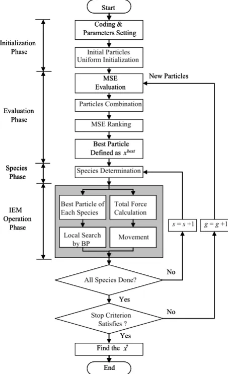
Figure 2: Description of SEMBP algorithm.
Initialization Phase
For SEMBP, each particle denotes a weighting vector
W=
[
ml,ml ,mr,mr ,σl ,σl ,σr ,σr ,γ ,ω ,ω ,c ,s]
T (11)which decides the dimension of problemD. In this paper, we used the good lattice point method which is one of the uniform methods to construct the uniform arrays [12]. If the randomly initialization is used, the statistical analysis is necessary, i.e., repetition training to get average performance should be done. In this paper, we adopt the uniform method to avoid the repetition training. Thus, we can reduce the computation complexity. In addition, the uniform method has less probability to produce the outliers which may affect the results deeply and avoids the particles crowding in a region.
The good lattice point method of uniform method provides a series of uniform arrays for different n and q. UN(qn)
denotes the uniform array and transforms into the initial particles. There are N rows in UN(qn) and each row represents
a particle in Rn. In the Initialization Phase, based on U N(qn), N
particles can be generated as follows:
⎥ ⎦ ⎤ ⎢
⎣ ⎡
− − + −
− +
= ( )
2 1 2 )
( 2
1 2
1 1 1
1 un ln
in n l l u i l
i x x
q u x x x q u x
x L (12)
where xi is the particles, xuk and xlk are the corresponding
upper bound and lower bound, uik is the element of UN(qn),
i=1, 2, …, N, and k=1, 2, …, n.
Evaluation Phase
This phase is used to calculate the fitness values of entire particles and compare the fitness values. We retain the particles which have better MSE among the particles of generation g and g+1. This process can guarantee the better performance. Another task in this phase is to remove the redundant particles which have similar fitness and locate in Particles Combination. It can improve the efficiency of SEMBP by removing the redundant particles. Since the similar particles may converge to the similar location, we remain the best particle among the similar particles. As a matter of fact, the redundant particles do not contribute further to the improvement of convergence. The conditions of particles combination are
th i
j i
s j
i
x x x
r x
x < × − <μ
) ( MSE
) ( MSE ) ( MSE and 1 . 0 ) , (
dis (13)
where dis(xi, xj) is the distance between xi and xj, rs is the
species radius, μth is the threshold and xi is the particle, i≠j.
Species Phase
The notion of species aims to identify multiple species via population and then determines a neighborhood best for each species. The dominating particle in each species is regarded as a neighborhood best called species seed. The species seed is always the fittest individual in the same species. All particles that fall within a distance from the species seed are classified as the same species. The definition of species depends on rs, which denotes the radius that measured by
distance from the center of a species to its boundary. Therefore, if rs is small, many isolated species would be
created in each generation. The small isolated particles species tend to prematurely converge to local minimum. If there are not sufficient numbers of particles in each species, the species will stop evolution. However, if rs is large, it is
possible to cover the entire variable range. In other words, the notion of species has no effect.
Subsequently, the particles in the population are sorted in decreasing order of fitness in MSE Ranking. As a matter of fact, the first particle in the ranking is the best-performing one and is denoted the species seed. The other particles in the population are checked in turn from best to worse and the particles whose distance between first species seed are smaller than rs are categorized into the first species. If the
particles do not fall within the radius of the first species seed, we select the particle which has minimum MSE to become a new species seed and the remaining particles are checked one by one that whether particles belong to the new species or not. Repeat the above steps until all particles are categorized. In this way, the species seeds and the number of species are generated in Species Phase.
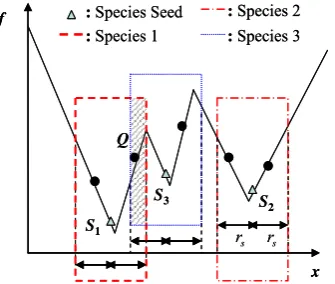
Figure 3 provides an example to illustrate the working of this phase. In the example, the algorithm locates three species and the particles S1, S2, and S3 are the species seeds. Note that
there is overlap between first species and third species. Hence, the prior identified species which center is S1 dominates the
S1
S2 S3
Q
x f
s
r rs
: Species Seed : Species 1
: Species 2 : Species 3
S1
S2 S3
Q
x f
s
r rs
: Species Seed : Species 1
[image:4.595.81.249.53.195.2]: Species 2 : Species 3
Figure 3: Example of how to determine the species in one- dimensioned problem.
IEM Operation Phase
There are three steps in the IEM operation phase: “Local Search of Best Particle by BP”, “Total Force Calculation,” and “Movement.” In order to improve the random process, we choose the step length λin Movement as one to accelerate the speed of convergence. After Species Determination, each sub-species proceeds Total Force Calculation and Movement which are the same as IEMBP’s. Nevertheless, in contrast to the complete population, the subpopulations have less computation complexity in determining the electromagnetic charge of each particle. In complete population, we should compute Ps×(Ps-1)×…×1 times of charges in Total Force
Calculation. But in the subpopulations, we only compute
∑
× − × ×S
s s p
p ( 1) L 1 times, where S is the number of species and ps is the number of particles in subpopulations.
And the best particle of sub-species processes local search by BP. In Local Search of Best Particle by BP, the gradient descent method is adopted to derive local search procedure of SEMBP for the aIT2FNS system. For clarification, we consider the single-output system and define the error cost function as
∑
=k
k e g
E ( )2
2 1 )
( (14) where e(k) y (k) yˆ(k) y (k) O(6)(k)
d
d − = −
= , g is the index of
generations, yˆ(k) and yd(k) are the aIT2FNS’s output and
desired output for discrete time k, respectively. By using the gradient descent method, the parameters updated law is described as
⎟ ⎠ ⎞ ⎜
⎝ ⎛
∂ ∂ − + = Δ + = +
W W
W W
W(g 1) (g) (g) (g) η E(g) (15)
where η is the learning rate. W=
[
W ,W ,γ ,Wω ,C]
T are theadjustable parameters, where C is the parameters of TSK layer, Wω is the consequent weights, W is the parameters
of lower MFs, W is upper MFs parameters and γ is the column vectors, i.e.,
[
]
Ts c
C= , (16)
[
l r l r]
Tω ω ω ω
ω =
W , (17)
[
l r l r]
Tm
m σ σ
=
W , (18)
[
ml mr σl σr]
T=
W . (19)
The update laws are similar to the results of [3]. For details, please refer to literature [3].
IV. SIMULATION RESULTS
We apply the aIT2FNS with SEMBP for chaotic system identification. Consider the chaotic system describes in [1]
0 . 1 ) 2 ( )
1 ( )
(k =−P⋅y2 k− +Q⋅y k− +
yd d d (20)
where P=1.4 and Q=0.3. For training the aIT2FNS system, we use the series-parallel learning scheme here. Herein, the inputs of the aIT2FNS are two input nodes for feeding the appropriate past values of yd(k-1) and yd(k-2), and the output of
the aIT2FNS yˆ(k) is the predicted result of system. The series-parallel training scheme is adopted as shown in Fig. 4. The approximated error is defined as follows
) ( ˆ ) ( )
(k y k y k
e ≡ d − . (21)
The following mean-square-error (MSE) is adopted to be the performance index
∑
=≡ T
k
k e T MSE
1 2( )
1 (22)
where T is the number of training pattern.
In this simulation, we use the good lattice point method to construct the uniform array. We use the initial array
) 61 ( 60 61
U to generate the initial parameters of aIT2FNS between [-1.5 1.5]. The learning rate of BP is selected to 0.1 and the threshold μth is selected to be 0.1. The initial
condition is [yd(1), yd(0)]T=[0.4, 0.4]T. Parameters of SEMBP
algorithm and aIT2FNS are chosen as in the following. - Rule number (R): 2
- Network structure (layer 1~ layer 6): (2-4-2-4-2-1) - Parameters number of aIT2FNS (D): 60
- Population size (Ps): 61
- Maximum generation (G): 20
Nonlinear System
RT2FNN-A
+
_
e u
Learning Algorithm
z-1
yˆ d y
Nonlinear System
aIT2FNS
+
_
e u
Learning Algorithm
z-1
yˆ d y
Nonlinear System
RT2FNN-A
+
_
e u
Learning Algorithm
z-1
yˆ
yˆ d
yd
y
Chaotic System
aIT2FNS
+
_
e u
Learning Algorithm
z-1
yˆ
yˆ d
yd
[image:4.595.324.531.451.636.2]y
Figure 4: Series-parallel identification scheme. The simulation results are described in Fig. 5 and Fig. 6. Figure 5(a) shows the phase plane of this chaotic system, whereas Figure 5(b) shows the identification result of aIT2FNS system. It can be observed that the SEMBP algorithm adjusts the parameters of aIT2FNS to predict system output accurately, and the aIT2FNS is similar to chaotic system. After training (20 generations), the MSE of aIT2FNS is 4.729×10⁻⁶, which is better than the best results
local minima. Obviously, the aIT2FNS system with SEMBP has better performance of accuracy, convergence and global optimum than the other algorithms. The final MFs are shown in Fig. 7(a)-(b). The constructed fuzzy rules are
1
R : IF x1 is 11
~
F and x2 is 21
~
F THEN
[
1.465 1.463] [
0.299 1.702] [
1 0.332 0.334]
2,1 x x
Y = − + + −
where ω=
[
−0.256 1.235]
and ω=[
-0.190 1.223]
.2
R : IF x1 is 12
~
F and x2 is 22
~
F THEN
[
0.236 0.947] [
1.783 0.404] [
1 0.776 2.224]
2,2 x x
Y = + − +
where ω=
[
−0.987 0.454]
and ω=[
−0.931 0.454]
.-1.5 -1 -0.5 0 0.5 1 1.5 -1.5
-1 -0.5 0 0.5 1 1.5
yd(k) yd
(k
-1
)
-1.5 -1 -0.5 0 0.5 1 1.5 -1.5
-1 -0.5 0 0.5 1 1.5
y(k)
y(
k-1)
[image:5.595.322.528.50.205.2](a) (b)
Figure 5: Phase plane plot of the example: (a) the chaotic system, (b) identification result of aIT2FNS.
Table 1 shows the comparison results of MSE in 20 training generations and the learning process is repeated for 20 runs. We can find that SEM takes 1665.1 second and EM takes 1306.1 second. It is obvious that SEM algorithm has better result than EM algorithm. Hence, we can know that using the species method has higher accuracy. In contrast with SEM and EM, SEMBP only takes 535.6 second which reduces the complexity of the calculation and promotes the simulated time efficiency. Although GA and PSO have similar computational complexity to SEMBP, but SEMBP has the better result. Referring to the Table 1, the MSE of SEMBP: 4.729×10⁻⁶ is smaller than those average MSEs of
SEM: 1.381×10⁻³; EM: 1.917×10⁻³; PSO: 7.291×10⁻⁴; GA:
8.420×10⁻⁴ and BP: 4.435×10⁻⁵.
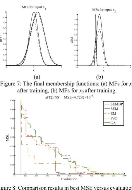
For the consideration of evaluations, Figure 8 shows the comparison results with different algorithms in the best MSE versus the evaluations. It can be seen that SEMBP does achieve better performance of MSE at the same evaluations. Thus, we can conclude that the SEMBP has the ability of high speed convergence, reduces the computational complexity and obtains global optimization.
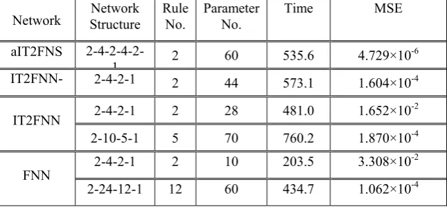
The simulation results with different networks are shown in Table 2. In this simulation, we make the dimension D as large as possible under the constraint expecting that the larger rule number will result in better performance. If we choose 5 rule numbers (70 parameters) in IT2FNN, there are 10 peak values of upper MFs are not adjusted, and the remaining 60 parameters just satisfy the uniform array (6160)
61
U . For the others which have less 60 parameters, we generate new uniform arrays by using different q. As we can see from Table 2, the network which has asymmetric type-2 MF is better than the others under the same rules. Due to the diversity of TSK, the aIT2FNS has more chance to get optimal solution. Obviously, the aIT2FNS with the TSK fuzzy rule and asymmetric MF has better performance than the other networks.
0 2 4 6 8 10 12 14 16 18 20 0
0.02 0.04 0.06 0.08 0.1 0.12 0.14 0.16
aIT2FNS MSE=4.7292×10⁻⁶
Generation
MSE
SEMBP SEM EM PSO GA BP
Figure 6: Simulation results: MSE in 20 generations. (−: SEMBP; −−: SEM; --: EM; −-: PSO; −−: GA; --: BP).
-5 0 5
0 0.1 0.2 0.3 0.4 0.5 0.6 0.7 0.8 0.9 1
x
μ
(x
)
MFs for input x1
-5 0 5
0 0.1 0.2 0.3 0.4 0.5 0.6 0.7 0.8 0.9 1
x
μ
(x
)
MFs for input x2
(a) (b)
Figure 7: The final membership functions: (a) MFs for x1
after training, (b) MFs for x2 after training.
0 100 200 300 400 500 600 700 800 900 1000 0
0.02 0.04 0.06 0.08 0.1 0.12 0.14 0.16
Evaluation
MS
E
aIT2FNS MSE=4.7292×10⁻⁶
[image:5.595.49.280.210.346.2]SEMBP SEM EM PSO GA
Figure 8: Comparison results in best MSE versus evaluations.
V. CONCLUSION
[image:5.595.312.538.237.562.2]global optimum. From the simulation results, we can observe that the proposed aIT2FNS with SEMBP algorithm has the ability of global optimization. And the simulation results also show that the aIT2FNS achieves better performance than the FNN, IT2FNN and IT2FNN-A systems. Performance comparisons with different categories of SEM, EM, PSO, GA and BP algorithms verify the effectiveness and efficiency of SEMBP. The example of chaotic system identification is proposed to show that SEMBP have the ability of global optimization and faster convergence.
REFERENCES
[1] C. H. Lee and C. C. Teng, “Identification and Control of Dynamic Systems Using Recurrent Fuzzy Neural Networks,” IEEE Trans. on
Fuzzy Systems, Vol. 8, No. 4, pp. 349-366, 2000.
[2] C. H. Lee and C. C. Teng, “Fine Tuning of Membership Functions for Fuzzy Neural Systems,” Asian Journal of Control, Vol. 3, No. 3, pp. 216-225, 2001.
[3] C. H. Lee and H. Y. Pan, “Performance enhancement for neural fuzzy systems using asymmetric membership functions,” Fuzzy Sets and
Systems, Vol. 160, No. 7, pp. 949-971, 2009.
[4] J. M. Mendel, Uncertain Rule-Based Fuzzy Logic Systems: Introduction
and New Directions, Upper Saddle River, Prentice-Hall, NJ, 2001.
[5] H. Hagras, “Type-2 FLCs: A New Generation of Fuzzy Controllers,”
IEEE Computational Intelligence Magazine, Vol. 2, No. 1, pp. 30-43,
2007.
[6] S. Horikawa, T. Furuhashi, and Y. Uchikawa, “On Fuzzy Modeling Using Fuzzy Neural Networks with the Back-propagation Algorithm,”
IEEE Trans. on Neural Networks, Vol. 3, No. 5, pp. 801-806, 1992.
[7] S. I. Birbil and S. C. Fang, “An Electromagnetism-like Mechanism for Global Optimization,” Journal of Global Optimization, Vol. 25, No.3, pp. 263-282, 2003.
[8] M. Clerc and J. Kenney, “The Particle Swarm-explosion, Stability, and Convergence in A Multidimensional Complex Space,” IEEE Trans. on
Evolutionary Computation, Vol. 6, No.1, pp. 58-73, 2002.
[9] D. E. Goldberg, Genetic Algorithms in Search, Optimization and
Machine Learning, Addison-Wesley, Reading, 1989.
[10] C. H. Lee, F. K. Chang, C. T. Kuo, and H. H. Chang, “A Hybrid of Electromagnetism-like Mechanism and Back-propagation Algorithms for Recurrent Neural Fuzzy Systems Design,” Int. J. of Systems Sciences, (Revised), Jan. 2010.
[11] J. R. Castro, O. Castillo, P. Melin, and A. R. Díaz, “A Hybrid Learning Algorithm for A Class of Interval Type-2 Fuzzy Neural Networks,”
Information Sciences, Vol. 179, No. 3, pp. 2175-2193, 2009.
[image:6.595.47.551.335.460.2][12] K. T. Fang, Number-theoretic Methods in Statistics, Chapman &Hall, 1994.
Table 1: Comparison results of average performance in MSE and computational complexity with uniform initialization for by using different algorithms (G=20, D=60, Ps =61).
Algorithm SEMBP SEM EM PSO GA BP
Average Time 535.6 1665.1 1306.1 544.4 539.0 36.4
Average MSE 4.729×10⁻⁶
1.381×10⁻³ 1.917×10⁻³ 7.291×10⁻⁴ 8.420×10⁻⁴ 4.435×10⁻⁵
Best MSE 2.435×10⁻⁴ 4.442×10⁻⁴ 9.136×10⁻⁵ 1.816×10⁻⁵
Worst MSE 3.939×10⁻³ 3.056×10⁻³ 3.913×10⁻³ 4.002×10⁻³
Table 2: Comparison results in parameter number, computational complexity and MSE with uniform initialization and SEMBP by using different network and rule number (G=20).
Network Structure Network RuleNo. ParameterNo. Time MSE aIT2FNS
2-4-2-4-2-1 2 60 535.6 4.729×10
-6
IT2FNN- 2-4-2-1 2 44 573.1 1.604×10⁻⁴
IT2FNN 2-4-2-1 2 28 481.0 1.652×10
-2
2-10-5-1 5 70 760.2 1.870×10⁻⁴
FNN 2-4-2-1 2 10 203.5 3.308×10
-2
[image:6.595.137.460.494.645.2]