via the R´
enyi Divergence of Optimized Orders
?Katsuyuki Takashima and Atsushi Takayasu??
Mitsubishi Electric, Japan
[email protected] The University of Tokyo, Japan
Abstract. In security proofs of lattice based cryptography, bounding the closeness of two probability distributions is an important procedure. To measure the closeness, the R´enyi divergence has been used instead of the classical statistical distance. Recent results have shown that the R´enyi divergence offers security reductions with better parameters, e.g. smaller deviations for discrete Gaussian distributions. However, since previous analyses used a fixed order R´enyi divergence, i.e., order two, they lost tightness of reductions. To overcome the deficiency, weadaptivelyoptimize the orders based on the advantages of the adversary for several lattice-based schemes. The optimizations enable us to prove the security with both improved efficiency and tighter reductions. Indeed, our analysis offers security reductions with smaller parameters than the statistical distance based analysis and the reductions are tighter than those of previous R´enyi divergence based analyses. As applications, we show tighter security reductions for sampling discrete Gaussian distributions with smaller precomputed tables for Bimodal Lattice Sig-nature Scheme (BLISS), and the variants of learning with errors (LWE) problem and the small integer solution (SIS) problem calledk-LWE andk-SIS, respectively.
Keywords: lattice based cryptography, tight reduction, R´enyi divergence, sampling discrete Gaussian, BLISS, LWE, SIS
1 Introduction
Background. The security of current cryptographic schemes relies on the hardness of the factor-ization/RSA problem and the (elliptic curve) discrete logarithm problem. Solving these problems becomes feasible when quantum computers are developed. Although quantum computers are not currently available, it is worthwhile to research next candidate cryptographic constructions. Lattice based cryptographic schemes have become central candidates for the post-quantum world. While some papers have focused on theoretical analyses, there are several papers that discuss practical implementations and the appropriate parameter selections [LP10, CN11, DDLL13, PDG14]. These works reveal some drawbacks in the efficiency of the lattice based schemes. For example, one of the deficiencies is the discrete Gaussian sampling with large deviations.
In security proofs of lattice based cryptography, bounding the closeness of two probability distributions (e.g., zero centered and non-zero centered discrete Gaussian distributions) is an im-portant procedure. To measure the closeness, the classical statistical distance (SD) is naturally used. However, several papers [LPR13, LSS14, LPSS14, BLL+15] used the R´enyi divergence (RD) [Ren61, EH12] instead of the SD. These works show that the RD offers better security reductions for
?
Date: 24 November, 2015. This paper is the full version of [TT15].
??The second author is supported by a JSPS Research Fellowship for Young Scientists. This work was supported by
lattice based cryptographic schemes. More concretely, the RD enables security reductions with bet-ter paramebet-ters (e.g. smaller deviations for discrete Gaussian distributions) that cannot be handled by the SD.
In short, the SD denotes differences of two probability distributions whereas the RD denotes the ratios of the distributions; hence, some properties of the SD expressed by additions are replaced by multiplications in the RD. For the SD based security proofs to be relevant, the quantity of the SD has to be smaller than a probability for an adversary to break the scheme. To satisfy the restriction, inefficient parameters (e.g. large deviations for discrete Gaussian distributions) have to be used. On the other hand, for the RD based security proofs to be relevant, the quantity of the RD can be permitted to larger bounds, e.g. the logarithm of the probability for an adversary to break the scheme. In some cases, the latter requirement (for the RD) is weaker than the former requirement (for the SD). Indeed, there are several reports confirming that the RD based analysis offers a significant parameter savings.
However, there is one disadvantage of the RD based analysis that cannot be disregarded; RD based security reductions lose the tightness. If the quantity of the SD is significantly small, the SD based security reduction becomes tight, and probabilities that an adversary will break the real and simulated schemes are almost identical. However, even if the value of the RD is significantly small, the probability that an adversary will break the real scheme is at least larger than the square root of the probability that an adversary will break the simulated scheme. Therefore, for the probability to break the real scheme to be sufficiently small, RD based analysis requires the probability to break the simulated scheme to be smaller than the SD based analysis. As a result, the RD based analysis sacrifices tightness to achieve the parameter saving compared with the SD based analysis.
Previous Results of RD Based Security Proofs. Suppose instances of a real cryptographic scheme are sampled from one distribution and instances of a simulated scheme are sampled from another distribution; the former (resp. latter) distribution is defined as thereal (resp.ideal) distri-bution. If the two distributions are statistically close, then an adversary that breaks the real scheme is also an adversary that breaks the simulated scheme. Then, if the simulated scheme is assumed to be secure, the real scheme is also secure.
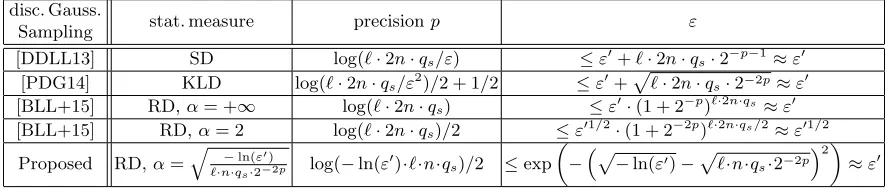
Table 1.Comparison of required precisionspand success probabilitiesεfor adversaries to break BLISS signatures where each Bernoulli variable is sampled with truncated probabilities (real distribution). Each signature is generated by sampling 2ndiscrete Gaussian variables, and each discrete Gaussian variable is produced by sampling`Bernoulli variables. Adversaries are allowed qs signing queries and break BLISS signatures with probabilities ε0 where each
Bernoulli variable is sampled with untruncated probabilities (ideal distribution). In the last column forε,≈is defined as the approximate equivalence when−ln(ε0)`·n·qs·2−2p, which holds for practical numerical examples given
in the right parameter of Table 4.
disc. Gauss.
Sampling stat. measure precisionp ε
[DDLL13] SD log(`·2n·qs/ε) ≤ε0+`·2n·qs·2−p−1≈ε0
[PDG14] KLD log(`·2n·qs/ε2)/2 + 1/2 ≤ε0+
p
`·2n·qs·2−2p≈ε0
[BLL+15] RD,α= +∞ log(`·2n·qs) ≤ε0·(1 + 2−p)`·2n·qs ≈ε0
[BLL+15] RD,α= 2 log(`·2n·qs)/2 ≤ε01/2·(1 + 2−2p)`·2n·qs/2≈ε01/2
Proposed RD,α=
q
−ln(ε0)
`·n·qs·2−2p log(−ln(ε
0
)·`·n·qs)/2 ≤exp
−p
−ln(ε0)−p
`·n·qs·2−2p
2 ≈ε0
Recently, Bai et al. [BLL+15] (Asiacrypt 2015) further improved the analysis based on the RD, however the reduction was no longer tight.
Boneh and Freeman [BF11] (PKC 2011) introduced thek-small integer solution (k-SIS) problem that is a variant of the small integer solution (SIS) problem [MR07]. In short, the k-SIS problem is defined as follows: given k hint vectors that are solutions to the original SIS problem and the goal of the problem is to compute the other SIS solution that is orthogonal to the k hint vectors. Based on the hardness of thek-SIS problem, Boneh and Freeman constructed lattice based linearly homomorphic signatures, k-time signatures, and proved that the k time GPV signature scheme [GPV08] is secure in the standard model. However, for thek-SIS problem to be no easier than the SIS problem, the solution bound of the SIS problem becomes exponential of k; hence, the k-SIS problem is as hard as the worst case standard lattice problems only when k = O(1). Ling et al. [LPSS14] (Crypto 2014) introduced the dual problem,k-learning with errors (k-LWE) problem that is a variant of the learning with errors (LWE) problem [Reg05]. Based on the hardness of the k-LWE problem, Ling et al. proposed the first algebraic construction of a traitor tracing scheme from lattices. Moreover, Ling et al. considered more efficient reductions than [BF11]. Their reduction enables the value of k to be a polynomial of the lattice dimension and the technique used in the reduction is applicable to the k-SIS problem. Specifically, Ling et al.’s reduction consists of two subreductions. In the first subreduction, LWE is reduced to k-LWE where k hint vectors are sampled from non-zero centered discrete Gaussian distributions (real distributions). In the second subreduction, the former k-LWE is reduced to k-LWE where k hint vectors are sampled from zero centered discrete Gaussian distributions (ideal distributions). To bound the closeness of two distributions, the RD is used. Although the analyses can handle smaller Gaussian deviations than the SD based analysis, the reduction is not tight.
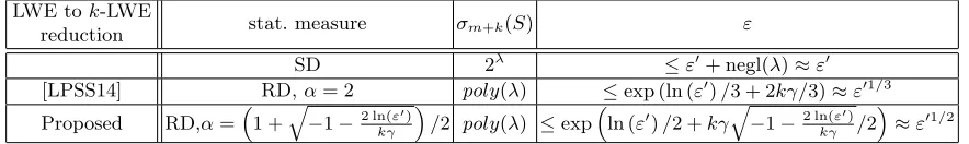
Table 2.Comparison of Gaussian deviations of hint vectorsσm+k(S) and success probabilitiesε for adversaries to
solve LWE. The quantity ofγ has a negative correlation with standard deviations of discrete Gaussian distributions. AdversariesAsolvek-LWE with advantageε0.λdenotes the security parameter and kdenotes the number of hint vectors. In the last column forε,≈is defined as the approximate equivalence when−ln(ε0)κγ.
LWE tok-LWE
reduction stat. measure σm+k(S) ε
SD 2λ ≤ε0+ negl(λ)≈ε0
[LPSS14] RD,α= 2 poly(λ) ≤exp (ln (ε0)/3 + 2kγ/3)≈ε01/3
Proposed RD,α=1 +
q
−1−2 ln(ε0)
kγ
/2 poly(λ) ≤expln (ε0)/2 +kγ
q
−1−2 ln(ε0)
kγ /2
≈ε01/2
Table 3.Comparison of Gaussian deviations of hint vectorsσm+k(S) and success probabilitiesε for adversaries to
solve SIS. The quantity ofγ has a negative correlation with standard deviations of discrete Gaussian distributions. Adversaries solvek-SIS with advantageε0.λdenotes the security parameter andkdenotes the number of hint vectors. In the last column forε,≈is defined as the approximate equivalence when−ln(ε0)κγ.
SIS tok-SIS
reduction stat. measure σm+k(S) ε
SD 2λ ≤ε0
+ negl(n)≈ε0 [LPSS14] RD,α= 2 poly(λ) ≤exp (ln (ε0)/2 +kγ)≈ε01/2
Proposed RD,α=p
−ln(ε0)/(kγ) poly(λ) ≤exp
−p
−ln(ε0)−√kγ2
≈ε0
– Sampling discrete Gaussian distributions for the BLISS signature scheme (Theorem 1 in Section 3) is achieved withbothreduced table storages and tight reductions. In particular, our analysis shows that the sampling can be performed with a 1276 bits table for BLISS-I scheme with 128 bit security. Table 1 compares the required precisions p(affecting table storages), and the probabilities ε0 (representing tightness) for an adversary to break the BLISS signature scheme with idealized distributions. Our reduction is as tight as the SD [DDLL13], KLD [PDG14], and RD of order +∞ [BLL+15] based analyses with reduced table storages. Although our table requires slightly larger storage than that of RD of order 2 based analysis [BLL+15], the reduction is tighter. See Table 4 in Section 3 for detailed comparisons.
– LWE tok-LWE reduction (Theorem 2 in Section 4) is achieved withbothsmall Gaussian devia-tions for sampling hint vectors and tighter reducdevia-tions. Table 2 compares the Gaussian deviadevia-tions σm+k(S), and the probabilities ε0 (that represent the tightness) for an adversary to solve k-LWE. Our reduction is as tight as the SD based analysis with smaller Gaussian deviations, and the deviations are as small as the previous RD based analysis [LPSS14] with tighter reductions. – SIS tok-SIS reduction (Theorem 4 in Section 5) is achieved withbothsmall Gaussian deviations for sampling hint vectors and tighter reductions. Table 3 compares the Gaussian deviations σm+k(S), and the probabilitiesε0 (that represent the tightness) for an adversary to solvek-SIS. Our reduction is as tight as the SD based analysis with smaller Gaussian deviations, and the deviations are as small as the previous RD based analysis with tighter reductions.
scheme. As the tables show, the RD based analyses (including previous works) offer security reduc-tions with smaller parameters (p for Table 1 and σm+k(S) for Tables 2 and 3) than the SD based analyses. Furthermore, our optimizations of the order offer tighter reductions than previous RD based analyses with fixed orders. Briefly speaking, although upper bounds ofεfor search problems (resp. distinguishing problems) are at least larger than ε01/2 (resp. ε01/3) when the order is fixed toα= 2, our improvements offer tighter upper bounds that are almost ε0 (resp. ε01/2). For appro-priate choices of parameters, our results offer almost the same tightness as the SD based analyses. Therefore, efficient parameters and tight reductions are compatible in our improved analyses.
Adaptive Optimization ofα. We briefly summarize the point of our improvements; theadaptive
optimization of the orderα. LetP and P0 be two computing problems where the problemP (resp. P0) is defined as follows: given X={xi:xi←Φ}i=1,...,k (resp.X0={x0i :xi0 ←Φ0}i=1,...,k) and the goal of the problem is to compute f(X) (resp.f(X0)). In cryptographic security proofs, P (resp. P0) can be viewed as the real (resp. simulated) cryptographic scheme, and Φ(resp. Φ0) is the real
(resp. ideal) distribution. Let γ be some quantity (that do not depend on α) that bounds the RD between the real distribution Φ and the ideal distribution Φ0 such that Rα(ΦkΦ0) ≤ exp(α·γ). Although there are no assurance for the upper bound of Rα(ΦkΦ0) to be O(exp(α)) for arbitrary distributions ΦandΦ0, it holds for the distributions that we study in this paper. By the definition and the properties of the RD, if there is an adversary A against the problem P with run-time T and advantage ε, then A is also an adversary against the problem P0 with run-time T0 =T and advantageε0 where
ε≤ε0·Rα(ΦkΦ0)k
α−1α ≤exp
α−1 α ·ln(ε
0) + (α−1)·kγ
(1)
where the second inequality is obtained from the factRα(ΦkΦ0)≤exp(α·γ), and kis the number of samples. We say that the reduction is tight when the right hand side of the inequality (1) is approximately equivalent toε0, i.e.,≈ε0. Since the number of samplesk(resp. the quantityγ) relate to cryptographic security or functionality, e.g., the number of signing queries in BLISS signatures, (resp. cryptographic efficiency, e.g., table storage size for sampling a discrete Gaussian distributions for BLISS signatures), we try to handle as largekandγ as possible. Then, the goal of our analysis is to prove the cryptographic security with both tight reductions and small parameters. When the order is fixed toα= 2 as previous works, the inequality (1) becomesε≤exp(ln(ε0)/2 +kγ); hence, even ifkand γ are small, the upper bound ofεbecomes larger thanε01/2 and the reduction is not tight. This is the disadvantage of previous RD based analyses that always lose the tightness.
To overcome the issue, weadaptivelyoptimize the order αto enable the reduction to be tighter. First, we analyze the inequality (1) with a generalα∈(1,+∞]. For the fixed analysis with α= 2, the tightness is lost by the existence of the exponent of ε0, α−α1. If a larger α is used, the ex-ponent becomes close to 1; therefore, the reduction is expected to be tighter. However, an in-finitely large α cannot be used since Rα(ΦkΦ0) becomes exponentially large, which results in a loss of the tightness. Hence, we optimize the order α to minimize the right hand side of the in-equality (1). The right hand side is bounded below by exp (ln(ε0)−kγ+ (−ln(ε0)/α+α·kγ))≥
expln(ε0)−kγ+ 2p−ln(ε0)·kγby the inequality of the arithmetic mean and geometric mean,
the orderα=p−ln(ε0)/(kγ), and the inequality (1) becomes
ε≤exp
ln(ε0)−kγ+ 2p−ln(ε0)·kγ= exp
−p−ln(ε0)−p
kγ2
. (2)
The right hand side of the inequality (2) is always smaller than that of the inequality (1) with fixed α = 2. Hence, our optimization always offers a tighter reduction than previous analyses [BLL+15, LPSS14]. Since we only consider the orderα∈(1,+∞], it leads toα=p−ln(ε0)/(kγ)>
1, i.e., −ln(ε0) > kγ. Moreover, when −ln(ε0) kγ, the right hand side of the inequality (2) is approximately equivalent to ε0; that is, the ideal P0 to the real P reduction is almost tight.
The above analysis captures security reductions for computing problems, a security proof for discrete Gaussian sampling and SIS to k-SIS reduction in our results. Although the result of the LWE to k-LWE reduction, which are distinguishing problems, does not follow the inequality (1), the spirit of the improvement is the same.
2 Preliminaries
Notation. Let ln(x) (resp. log(x)) denote the natural logarithm (resp. the base 2 logarithm) of x. Let T denote the additive group R/Z. For an integer q, we let Zq denote the ring of integers modulo q. Vectors are denoted in bold and are column representations. For b ∈ Rn, we let kbk
denote its Euclidean norm. We let h·,·i denote the canonical inner product. If A is a matrix, its entries are denote byaij. For two matricesAand B of compatible dimensions, we let (A|B) (resp. (AkB)) denote the horizontal (resp. vertical) concatenations ofA andB. ForA∈Zmq×n, we define Im(A) ={As:s∈Zn
q} ⊆Zmq . ForX⊆Zmq , we let Span(X) denote the set of all linear combinations of elements ofX. We letX⊥denote the linear subspace{b∈Zm
q :∀c∈X,hb,ci= 0}. For a matrix S ∈Zm×n, we letkSk denote the norm of its largest column. The smallest (resp. largest) singular value ofS is denoted byσn(S) = inf(kSuk) (resp.σ1(S) = sup(kSuk)) whereu∈Rn andkuk= 1.
If D is a probability distribution, we let Supp(D) = {x :D(x) 6= 0} denote its support. The uniform distribution on a finite set X is denoted by U(X). The statistical distance (SD) between two distributionsD1 andD2 over a countable supportXis given by∆(D1, D2) = 12Px∈X|D1(x)− D2(x)|. For a function f :X → Rover a countable domain X, we letf(X) = Px∈Xf(x). Letνβ denote the one-dimensional Gaussian distribution onT with center 0 and standard deviationβ.
Lattices and Discrete Gaussian Distributions. Lattice Λ is an additive discrete subgroup of
Rn. An n-dimensional lattice Λ⊆Rn is the set of all integer linear combinationsPkj=1cjbj where cj ∈ Z of some linearly independent vectors b1, . . . ,bk ∈ Rn for some k ≤n. The rank of Λ is k.
The determinant det(Λ) is defined by pdet(BTB), where B = (b
i)i is any such basis of Λ. For a matrix A ∈ Zm×n
q , define Λ⊥(A) = {x ∈ Zm :xT ·A = 0 mod q}. The dual Λ∗ of a lattice Λ is defined byΛ∗ ={x∈Rn:∀y∈Λ,hx, yi ∈Z}.
For a rank-nmatrixS∈Rm×n and a vectorc∈
Rn, the ellipsoid discrete Gaussian distribution
with parameterSand centercis defined as follows:∀x∈Rn, ρ
S,c(x) = exp
−π(x−c)T STS−1
(x−c). Note thatρS,c(x) = exp(−πk(ST)†(x−c)k2), where X† denotes the pseudo-inverse ofX. The
ellip-soid discrete Gaussian distribution over a cosetΛ+z of a lattice Λ, with parameter S and center
cis defined as follows: ∀x∈Λ+z, DΛ+z,S,c(x) = ρS,c(x)/ρS,c(Λ). ForS =sIm, we write ρs,c and
Smoothing Parameter. The smoothing parameter [MR07] ηε(Λ) of an n-dimensional lattice Λ for real ε > 0 is defined as the smallest s such that ρ1/s(Λ∗\ {0}) ≤ ε. When the deviation of the discrete Gaussian distribution is larger than the smoothing parameter, the following results are known.
Lemma 1 (Lemma 2.5 of [LSS14]) Let Λ be an n-dimensional lattice and ε∈(0,1). Then for anyc∈Rn and s≥η
ε(Λ) we have ρs,c(Λ)∈[1−ε,1 +ε]·det(Λ)−1.
Lemma 2 (Lemma 3 of [AGHS13]) For a rank-n lattice Λ, a constant 0 < ε < 1, a vector
c and a matrix S with σn(S) ≥ ηε(Λ), if x is sampled from DΛ,S,c then kxk ≤ σ1(S) √
n with probability ≤ 1+ε
1−ε·2
−n.
Lemma 3 (Lemma 1 of [LPSS14]) Let q be a prime,mandnbe integers withm≥2nandε > 0. Then ηε(Λ⊥(A))≤4qn/m
p
log(2m(1 + 1/ε))/π, for all except a fraction2−Ω(n) of A∈Zm×n q .
R´enyi Divergence. For any two discrete probability distributionsP and Qsuch that Supp(P)⊆
Supp(Q) andα∈(1,∞], we define the R´enyi divergence (RD) of order α by
Rα(PkQ) =
X
x∈Supp(P)
P(x)α Q(x)α−1
1 α−1
forα∈(1,∞), R∞(PkQ) = max
x∈Supp(P)
P(x) Q(x).
We summarize the basic properties of the RD that we use in this paper.
Lemma 4 (Lemma 4.1 of [LSS14]) Let P1, P2, P3 and Q1 and Q2 denote discrete distributions on a domain X. Let α∈(1,+∞]. Then the following properties hold:
– Log. Positivity: Rα(P1kQ1)≥Rα(P1kP1) = 1. – Data Processing Inequality: Rα
P1fkQf1 ≤ Rα(P1kQ1) for any function f, where P1f(resp.
Qf1) denotes the distribution off(y) induced by sampling y←P1(resp. y←Q1).
– Multiplicativity: LetP andQdenote any two distributions of a pair of random variables(Y1, Y2) on X ×X. For i ∈ {1,2}, let Pi(resp. Qi) denote the marginal distribution of Yi under P
(resp. Q), andP(2|1)(·|y1) (resp.Q(2|1)(·|y1)) denote the conditional distribution ofY2 given that
Y1 =y1. Then we have Rα(PkQ) =Rα(P1kQ1)·Rα(P2kQ2) if Y1 andY2 are independent, and
Rα(PkQ)≤R∞(P1kQ1)·maxy1∈XRα(P2|1(·|y1)kQ2|1(·|y1)).
– Weak Triangle Inequality: We have Rα(P1kP3)≤Rα(P1kP2)·R∞(P2kP3), and Rα(P1kP3)≤
R∞(P1kP2)α/(α−1)·Rα(P2kP3).
– R∞Triangle Inequality: IfR∞(P1kP2)andR∞(P2kP3)are defined, thenR∞(P1kP3)≤R∞(P1kP2)·
R∞(P2kP3).
– Probability Preservation: LetE⊆Xbe an arbitrary event. ThenQ1(E)≥P1(E)α/(α−1)/Rα(P1kQ1).
The divergenceR1is the exponential of the KLD,R1(PkQ) = exp
P
x∈Supp(P)P(x) log
P(x)
Q(x)
. The probability preservation property of the KLD can be written asQ(E)≥P(E)−plnR1(PkQ)/2.
In this paper, we use the following result1 that is essential for our improvements in Sections 4 and 5.
1In the proceedings version of [BLL+15], Bai et al. showed a slightly better bound for our Lemma 5. However, we
Lemma 5 For any n-dimensional lattice Λ ⊆ Rn and inversible rank-n matrix S ∈
Rm×n for
m≥n, set P =DΛ,S,c andQ=DΛ,S,c0 for some fixed c,c0∈Rn. If c,c0 ∈Λ, let ε= 0; otherwise,
fix ε∈(0,1)and assume that σn(S)≥ηε(Λ). Then Rα(PkQ)≤1+1−εε
α α−1
·exp
απkσc−c0k2
n(S)2
.
3 Tighter Analysis for Discrete Gaussian Sampling with Small Precomputed Tables
In this section, we study Ducas et al.’s discrete Gaussian sampling [DDLL13] with precomputed tables. By adaptively optimizing the order of the RD, we show that the sampling for BLISS signature scheme can be securely performed with less table storage.
Discrete Gaussian Sampling. In the BLISS signature scheme [DDLL13], signing a message requires sampling 2n independent integers from one-dimensional discrete Gaussian distributions DZ,s, where s is the standard deviation parameter. See Appendix B for detailed algorithms. In [DDLL13], an efficient sampling algorithm forDZ,sis presented. LetBcbe the Bernoulli distribution that outputs 1 with probabilitycand 0 otherwise. First, the algorithm samples`Bernoulli random variables of the formBci fori= 0, . . . , `−1 whereci = exp(−π2
i/s2). By using a rejection sampling
[GPV08], these `Bernoulli samples produce a sample fromDZ,s. Hence, to sign a signature,`·2n Bernoulli variables are sampled. For the detailed algorithm, see Table 3 in [DDLL13]. In this paper, we focus on sampling from Bernoulli distributions. To efficiently sample the Bernoulli random variables, a precomputed table that stores the probabilities ci for i = 0, . . . , `−1 is used. The algorithm samplesxfrom a uniform distribution over (0,1), and outputs 1 ifx < ciand 0 otherwise. Since the exact quantities ofciare real, the truncated values ˜ci=ci+εiare stored. Here,|εi| ≤2−pci denotes the truncation error where p is the bit precision. When ci >1/2, truncated probabilities are stored for 1−ci with the bit precisionsp. Hence, the table storage becomes`·pbits whose size affects the efficiency.
Previous Analyses. As in [BLL+15], we analyze the security of BLISS when an adversary is allowed up to qs signing queries. In this case, `·2n·qs Bernoulli random variables are sampled since we should sample `·2n Bernoulli random variables to sign a signature. Let Φ (resp. Φ0) be a distribution of signatures in the view of the adversary where all `·2n·qs variables are sampled from the truncated (resp. untruncated) Bernoulli distribution B˜ci (resp. Bci). The distribution Φ
(resp. Φ0) is regarded as the real (resp.ideal) distribution. We will show that the BLISS signature scheme by sampling from the real distributionΦis secure with smaller parameters, i.e., more signing queriesqs and less bit precision p, and the reduction from the scheme by sampling from the ideal distributionΦ0 is tight, i.e.,εbecomes small with larger ε0.
To examine the security, Ducas et al. [DDLL13] and P¨oppelmann et al. [PDG14] used the SD and KLD, respectively. Although we omit the details, the SD becomes∆(Φ, Φ0) =`·2n·qs·2−p−1, which leads toε≤ε0+`·2n·qs·2−p−1; hence, when p≥log(`·2n·qs/ε), the reduction becomes almost tight, i.e., ε ≤ 2·ε0. The KLD becomes lnR1(ΦkΦ0) ≤ `·2n·qs ·2−2p that leads to
Bai et al. [BLL+15] used the RD of orders α = +∞ and 2, and showed that the sampling algorithm becomes secure with less table storage `·p, which does not depend on ε. From the multiplicativity property over i = 0, . . . , ` −1 and the data processing inequality of the RD, Rα(ΦkΦ0) ≤ (maxi∈[1,`]Rα(Bc˜ikBci))
`·2n·qs. Let ε (resp. ε0) be the advantage for an adversary to
break BLISS whose instances are sampled from Φ (resp. Φ0). From the probability preservation property of the RD,ε≤(ε0·Rα(ΦkΦ0))
α−1 α .
Using symmetry, we assume thatci ≤1/2; otherwise, we exchange ci and 1−ci in the following calculations. First, Bai et al. used the RD of order α= +∞. By definition,
R∞(Bc˜ikBci) = max
ci+εi ci ,
1−ci−εi 1−ci
= 1 +|εi|
ci ≤1 + 2
−p.
Then, R∞(ΦkΦ0) ≤ (1 + 2−p)`·2n·qs from the multiplicativity property over i = 0, . . . , `−1 and
the data processing inequality of the RD. The RD bound implies ε ≤ ε0 ·(1 + 2−p)`·2n·qs from
the probability preservation property of the RD. Hence, when p ≥ log(`·2n·qs), the reduction becomes almost tight, i.e., ε ≤ 2 ·ε0. Since the probability preservation property of the RD is multiplicative, the required precisions do not depend onε, which results in less table storage. The required precision is less than that of the previous SD and KLD based analyses [DDLL13, PDG14].
Next, the RD of order α∈(1,+∞) was considered. By definition,
(Rα(Bc˜ikBci))
α−1=c
i
ci+εi ci
α
+ (1−ci)
1−ci−εi 1−ci
α
. (3)
In particular, Bai et al. focused on the caseα= 2, which is, R2(B˜cikBci) = 1 +
ε2 i
ci(1−ci) ≤1 + 2
−2p. The last inequality holds by using the fact that |εi| ≤ 2−pci and the assumption ci ≤1/2. Then, R2(ΦkΦ0) ≤ (1 + 2−2p)`·2n·qs from the multiplicativity property over i = 0, . . . , `− 1 and the
data processing inequality of the RD. The RD bound leads to ε ≤ ε01/2 ·(1 + 2−2p)`·2n·qs from
the probability preservation property of the RD. Hence, Bai et al. concluded the precision to be p≥log(`·2n·qs)/2. The required precision of the R2 based analysis is half that of theR∞ based
analysis. The improvements are derived from the exponent of R2(B˜cikBci), which becomes −2p,
although that of R∞ is −p. Although the required precision is less than that of the R∞ based
analysis, R2 based analysis offers a reduction that is no longer tight, i.e., ε ≤ 2·ε01/2 from the
probability preservation property of the RD. The deficiency comes from the preservation property ofR2, i.e.,ε≤ε01/2·R2(ΦkΦ0). The exponent ofε0 never allows tight reductions even if the precision
become infinitely large.
Tighter RD Based Analysis with Smaller Table Storage. In the rest of this section, we show that theRαbased analysis offers both less required precision and tighter reductions when the order α is appropriately determined. First, the RD of the inequality (3) is bounded for generalα as follows.
Lemma 6 Let probability distributionsB˜ci andBci be defined as above. If the order αis an integer
with α <2p, then (Rα(B˜cikBci))
α−1 = expα(α−1) 2 ·2
−2p+O((α2−p)3).
For the condition in Theorem 1, we define the minimal key recovery advantage ˆε. In Appendix A of [DDLL13], known attacks for BLISS are summarized including lattice reduction attacks for the underlying SIS, primal and dual lattice reduction key recoveries. The most primitive brute-force key recovery is also analyzed, where an adversary guesses a random secret vector g and checks whetherf =a−q1(2g+ 1) modq is a legitimate secret polynomial or not for the public polynomial aq; otherwise, the adversary aborts. The advantage is estimated as2 εˆ= 2−d1−d2 · n
d1
−1 · n−d1
d2
−1
where d1 and d2 are defined in the key generation of BLISS. For example, ˆε ≈2−600 for BLISS-I
parameters n= 512, d1 ≈ 153, and d2 ≈ 0. In Theorem 1, we consider powerful adversaries with
signing query number qs≈264. For such a powerful adversary, it holds that`·n·qs −ln(ˆε). For example, for practical BLISS-I parameters (n= 512, `= 29), the left (resp. right) hand side ≈278 (resp. ≈600), then the above inequality holds.
Theorem 1 Let parametersp, `, n, and qs that satisfy `·n·qs −ln(ˆε), and probability distribu-tionsB˜ci andBci be defined as above. Then, if there is an adversaryAagainst the BLISS signature
scheme when Bernoulli random variables are sampled from Bc˜i with run-time T and advantageε,
thenA is also an adversary against the BLISS signature scheme when Bernoulli random variables are sampled fromBci with run-time T
0 =T and advantage ε0 that satisfies−ln(ε0)> `·n·q
s·2−2p
and
ε≤exp
−p−ln(ε0)−p`·n·qs·2−2p2
. (4)
Proof. To prove the theorem, we consider the RD of order α that is much smaller than 2p. (The fact is justified by the inequality `·n·qs −ln(ˆε) later in this proof. ) By Lemma 6, we ignore the small term and assume (Rα(B˜cikBci))
α−1 = expα(α−1) 2 ·2
−2p, which implies
(Rα(ΦkΦ0))α−1 ≤(Rα(Bc˜ikBci))
(α−1)·`·2n·qs = exp α(α−1)·`·n·qs·2−2p
from the multiplicativity property over i= 0, . . . , `−1 and the data processing inequality of the RD. Since the exponent is −2p, the analysis requires a small precision similar to the R2 based
analysis. Furthermore,
ε≤ ε0·Rα(ΦkΦ0)
α−1 α = exp
α−1 α ln(ε
0
) + (α−1)·`·n·qs·2−2p
holds from the probability preservation property of the RD. The inequality is equivalent to the inequality (1) in Section 1. The right hand side of the inequality is bounded below by
exp ln(ε0)−`·n·qs·2−2p+ −ln(ε0)/α+α·`·n·qs·2−2p
≥exp
ln(ε0)−`·n·qs·2−2p+ 2p−ln(ε0)·`·n·qs·2−2p
by the inequality of the arithmetic mean and geometric mean; the equality holds if and only if
−ln(ε0)/α=α·`·n·qs·2−2p, i.e., α=
q
−ln(ε0)
`·n·qs·2−2p. 2
In [DDLL13], thebrute-forceadversary for all key candidates is considered; however, we consider the corresponding
Table 4.Comparison of required precisionsp, table bit-size and upper bounds of−logε0. The left table is a summary of previous analyses that are the same as in Table 1 of [BLL+15]. The right table is based on our analysis.
statistical measure p Table bit-size−logε0 SD [DDLL13] 207 6003 ≤129 KLD [PDG14] 168 4872 ≤129
RD,α= +∞[BLL+15] 79 2291 ≤129 RD,α= 2 [BLL+15] 40 1160 256.45
α p Table
bit-size −logε
0
2.48 36 1044 418.66 6.94 38 1102 184.97
24.76 40 1160 141.26 96.07 42 1218 131.25 381.30 44 1276 128.80
Notice that the order α =
q
−ln(ε0)
`·n·qs·2−2p satisfies our assumption α 2
p. By definition, the inequality ˆε≤ ε0, which is equivalent to −lnε0 ≤ −ln(ˆε), holds. Since we only consider the case
−ln(ˆ)`·n·qs,−ln(0)`·n·qs also holds. That leads toα=
q
−ln(ε0)
`·n·qs·2−2p 2
p. Next, we set the order α=
q −
ln(ε0)
`·n·qs·2−2p. In this case, the above inequality becomes
ε≤exp
−p−ln(ε0)−p`·n·qs·2−2p2
.
The inequality is equivalent to the inequality (2) in Section 1 as required. The orderα=
q
−ln(ε0)
`·n·qs·2−2p
that is used satisfies α∈(1,+∞] since−ln(ε0)> `·n·qs·2−2p. ut For the BLISS signature scheme to be secure, i.e., εto be small, with smaller −ln(ε0) (larger ε0, i.e., tighter reductions), more signing queries qs (i.e., for powerful adversaries), and larger 2−p (less precisionp, i.e., more efficiency), the inequality (4) shows an appropriate trade-off. The upper bound ofεbased on our analysis is lower than that of Bai et al.’sR2 based analysis for allε0, `, n, qs,
and p. In particular, from the inequality (4), if
ε≤exp
−p−ln(ε0)−p`·n·q
s·2−2p
2
=ε0·exp2p−ln(ε0)·`·n·q
s·2−2p−`·n·qs·2−2p
,
when−ln(ε0)·`·n·qs·2−2p≤1, thenε≤ε0·O(1) holds and the upper bound cannot be obtained by theR2 based analysis. The condition leads to the precision requirementp≥log(−ln(ε0)·`·n·qs)/2 that is less than that of the SD, KLD, andR∞based analyses for powerful adversaries, i.e.,`·n·qs −ln(ˆε).
Numerical Examples. Table 4 shows the numerical examples that compare required precisionsp, table bit-size`·p, and upper bounds of −log(ε0) of previous analyses [DDLL13, PDG14, BLL+15] and our analysis. According to Table 1 in [BLL+15], an adversary is allowedqs= 264 sign queries and breaks BLISS-I with probability ε= 2−128 with parameters n= 512,and `= 29. The values of −log(ε0) are given by
−log(ε0)≤log(e)·p−ln(ε) +p`·n·qs·2−2p
which is equivalent to the inequality (4). The table clarifies our improvements that are briefly summarized in Table 1. Although Bai et al.’s R2 based analysis [BLL+15] requires less precision
p than SD, KLD, andR∞ based analyses [DDLL13, PDG14, BLL+15], the reduction is no longer
tight and −log(ε0) becomes much larger than −log(ε) = 128. Theorem 1 shows a better trade-off than previous analyses. As the right table indicates, as the bit precision p increases, −log(ε0) becomes smaller, which makes the reduction tighter. In particular, based on our analysis, the upper bound of −log(ε0) forp = 40 is smaller that of theR2 based analysis by Bai et al. [BLL+15]. As
a result3 , whenp≥44, the reduction becomes almost tight, i.e., −log(ε0)≤129. Notice that the ordersα are always much smaller than 2p, which we assume to bound the quantity of RD.
4 Tighter Analysis for LWE to k-LWE Reduction
In this section, we study LWE tok-LWE reduction [LPSS14]. By adaptively optimizing the order of the RD, the reduction becomes tighter.
First, we introduce a variant of the LWE problem, where the number of samples m produced by the oracle is a priori bounded.
Definition 1 (LWEβ,m Problem) Given A← U Zmq ×n
, the goal of the LWEβ,m problem is to
distinguish between the distributions (over Tm)
1
qU(Im(A)) +ν m β and
1 qU Z
m q
+νβm.
Next, we introduce the k-LWE problem defined in [LPSS14].
Definition 2 ((k, S, C)-LWEβ,m Problem, Definition 7 of [LPSS14]) Let k≤m, S ∈Rm×m be invertible andC = (c1k · · · kck)∈Rk×m. GivenA←U Zmq×n
,andxi←DΛ⊥(A),S,c
i fori≤k,
the goal of the(k, S, C)-LWEβ,mproblem (the(k, S)-LWEβ,m problem whenC = 0) is to distinguish between the distributions (over Tm)
1
qU(Im (A)) +ν m β and
1 qU
Spani≤k(xi)⊥
+νβm.
The k vectors x1, . . . ,xk can be used to solve the original LWEβ,m. When we obtain a vector y from the left distribution, hxi,yi becomes much smaller than 1 for standard parameter settings sincexi ∈Λ⊥(A) and is orthogonal to Im(A). On the other hand, when we obtain a vectory from the right distribution,hxi,yiis uniform. However, (k, S, C)-LWEβ,mbecomes non-trivial and seems to be hard since the right distribution 1qU Zmq
is replaced by 1qU
Spani≤k(xi)
⊥
.
Ling et al. [LPSS14] proved the security reduction for the (k, S)-LWEβ,mproblem. An adversary that solves the (k, S)-LWEβ0,m+k problem in Definition 2 is also an adversary that solves the
LWEβ,m problem in Definition 1. However, Ling et al.’s reduction is not tight since they fix the order of the RD toα= 2. We show the tighter security reduction as follows byadaptivelyoptimizing the order.
3
In [BLL+15], Bai et al. analyzed the precisions by measuring the closeness between B˜ci and Bci which depend
Theorem 2 Letm, q, σ, σ0,andksatisfyσ≥Ω(max(m√logm, σ0k/(m+k))), σ0 ≥Ωm3σ2log3/2(mσ),
q ≥ Ω σ0√logm is prime, and m ≥ Ω(nlogq). Then there exists a probabilistic polynomial-time reduction from A0 for LWEβ,m in dimension n to (k, S)-LWEβ0,m+k in dimension n, where
β0 =Ω m3/2σ0β
,S is a diagonal matrix,aii=σfor1≤i≤m, andaii=σ0 form+1≤i≤m+k.
More concretely, using a (k, S)-LWEβ0,m+k algorithm with run-time T and advantage ε, the
re-duction gives anLWEβ,malgorithm with run-timeT0=O T·poly(m)·(ε−2−Ω(n))−2log((ε−2−Ω(n))−1)
and advantage ε0 where
ε≤exp ln ε
0+ 2−Ω(n)
2 +
p
−1−2nln(ε0+ 2−Ω(n))
2n
!
·2O(k·2−n)+ 2−Ω(n).
In [LPSS15], Ling et al. suggested appropriate selections of parameters as k = m/10, σ = ˜
Θ(n), σ0= ˜Θ(n5), q= ˜Θ(n5) and m=Θ(nlogn).
Proof. The proof of Theorem 2 consists of Lemma 7 and Theorem 3; that is, the required reduction of Theorem 2 consists of two subreductions as in [LPSS14]. The first is the LWE to (k, S, C)-LWE reduction, and the second is the (k, S, C)-LWE to (k, S)-LWE reduction. We follow the first subreduction.
Lemma 7 ([LPSS15]) Let parametersk, n, m, q, σ, σ0, β0, and matrix S be defined as in Theorem 2. Let C∈Rk×(m+k) be the matrix whose i-th row is the unit vector c
i = (0m|δi) where δi denotes
the i-th canonical unit vector in Zk for k = 1, . . . , k. If there exists a distinguisher A against
(k, S, C)-LWEβ0,m+kin dimensionnwith run-timeT and advantageε, thenAis also a distinguisher
againstLWEβ,m in dimension nwith run-time T0=T+poly(m) and advantage ε0 =ε−2−Ω(n). Next, we analyze the second subreduction. Although our analysis is similar to that in [LPSS14], the following Theorem 3 is obtained as an application of our optimized selection of the orderα.
Theorem 3 Let m0 =m+k and assume thatσm0(S)≥ω(
√
n). Let γ be a constant that satisfies
σm0(S) ≥ pπ/γ· kCk. If there exists a distinguisher A against (k, S)-LWEβ0,m0 in dimension n0
with run-time T and advantage ε, then there exists a distinguisher A0 against (k, S, C)-LWE
β0,m0
with run-time T0 = O
poly(m0)· ε−2−Ω(n)−2·T ·log ((ε−2−Ω(n))−1)
and advantage ε0 that
satisfies−ln ε0+ 2−Ω(n)≥kγ, and
ε≤exp ln ε
0+ 2−Ω(n)
2 +
kγp−1−2 ln(ε0+ 2−Ω(n))/(kγ)
2
!
·2O(k·2−n)+ 2−Ω(n).
The proof of Theorem 3 is given in Appendix D. Based on the SD, the deviations to sample k hint vectors become exponentials of the security parameter. Since Ling et al. used the RD, the deviations become smaller. Moreover, we optimize the orderα and obtain a tighter reduction.
Note that in the above reduction from LWEβ,mto (k, S, C)-LWEβ0,m+k,kCk= 1 andσm0(S) =
σ =Ω(n); hence, we set γ =O(1/n2). Using the fact thatk < n and we can obtain the required
Analogous to Theorem 3, the inequality in [LPSS14] can be written as
ε≤exp ln ε
0+ 2−Ω(n)
3 +
2kγ 3
!
·2O(k·2−n)+ 2−Ω(n).
The inequality can be obtained by R2. The right hand side of the inequality becomes the same as
ours only whenα= 2; otherwise, our analysis always offers a tighter reduction since the right hand side of the inequality in Theorem 3 is always smaller than that of Ling et al.
5 Tighter Analysis for SIS to k-SIS Reduction
In this section, we study SIS to k-SIS reduction [BF11, LPSS14]. By adaptively optimizing the order of the RD, the reduction becomes tighter.
First, we introduce the SIS problem.
Definition 3 (SISβ,m Problem) Given A←U Zmq×n
, the goal of theSISβ,m problem is to find
a nonzero vector b∈Zm such that
– kbk ≤β,
– bT ·A=0 mod q.
Next, we introduce the k-SIS problem. The definition follows from Definition 2 rather than the original definition from [BF11].
Definition 4 ((k, S, C)-SISβ,m Problem, Adapted from Definition 4.1 of [BF11]) Let k ≤ m, S ∈ Rm×m be invertible, and C = (c1k · · · kck) ∈ Rk×m. Given A ← U Zmq×n
and xi ← DΛ⊥(A),S,c
i for i ≤ k, the goal of the (k, S, C)-SISβ,m problem (the (k, S)-SISβ,m problem when
C= 0) is to find a nonzero vector b∈Zm such that
– kbk ≤β,
– bT ·A=0 mod q, – b∈Spani≤k(xi)⊥.
The k vectors x1, . . . ,xk for (k, S)-SISβ,m can be used to solve the original SISβ,m. By definition, the vectors satisfy the second condition of SISβ,m. Since the vectors are sampled from Gaussian distributions, their norms are small and the vectors are expected to satisfy the first condition of SISβ,m. However, (k, S, C)-SISβ,mis non-trivial and seems to be hard since the additional condition
b∈Spani≤k(xi)
⊥
have to be satisfied. The integer linear combinations of thekhint vectors cannot be solutions to the (k, S, C)-SISβ,m.
Ling et al. [LPSS14] briefly summarized the SIS to k-SIS reduction. As the LWEβ,m to the (k, S)-LWEβ,m+kreduction, they showed that an adversary that solves the (k, S)-SISβ0,m+kproblem
in Definition 4 is also an adversary that solves the SISβ,m problem in Definition 3. However, Ling et al.’s reduction is not tight since they fix the order of the RD to α = 2. We show the tighter security reduction as follows byadaptively optimizing the order.
then A0 is also an adversary against SIS
β,m in dimension n and β = Ω(
√
kmσ0β0) with run-time
T0 =T+poly(m) and advantage ε0 where
ε≤exp
−q−ln ε0+ 2−Ω(n)
−√kγ
2
·2O k·2−n
+ 2−Ω(n).
Proof. As LWE to (k, S)-LWE reduction, the reduction consists of two subreductions. The first is the SIS to (k, S, C)-SIS reduction, and the second is the (k, S, C)-SIS to (k, S)-SIS reduction. The first subreduction is almost identical to that of the LWE to (k, S, C)-LWE reduction as suggested in [LPSS14].
Lemma 8 (Adapted from [LPSS14]) Let k, n, m, q, σ, and σ0 be the same as those in The-orem 2. Let matrices C and S be the same as Lemma 7. If there exists an adversary against
(k, S, C)-SISβ0,m+k in dimension n, with S as in Theorem 2, run-time T, and advantage ε, then
there exists an adversary against SISβ,m in dimension n with β = Ω(
√
kmσ0β0), run-time T0 = T+poly(m), and advantage ε0=ε−2−Ω(n).
The proof of Lemma 8 is given in Appendix E.
Next, we analyze the second subreduction. The following Theorem 5 is obtained as an application of our optimized selection of the order α. We cannot obtain the same tightness when we fix the order α= 2 as in [LPSS14].
Theorem 5 Assume thatσm0(S)≥ω(
√
n). Letγ be a constant that satisfiesσm0(S)≥
p
π/γ·kCk. If there exists an adversaryAagainst(k, S)-SISβ,m0 in dimensionnwith run-timeT and advantage
ε, thenAis also an adversary against (k, S, C)-SISβ,m0 with run-timeT0 =T and advantageε0 that
satisfies−ln ε0+ 2−Ω(n)≥kγ, and
ε≤exp
−q−ln ε0+ 2−Ω(n)
−√kγ
2
·2O k·2−n+ 2−Ω(n).
The proof of Theorem 5 is given in Appendix E. Based on the SD, the deviations to sample k hint vectors become exponentials of the security parameter. Since Ling et al. used the RD, the deviations become smaller. Moreover, we optimize the orderα and obtain a tighter reduction.
Note that in the above reduction from SISβ,m to (k, S, C)-SISβ0,m+2n,kCk= 1, and σm0(S) =
σ =Ω(n). Hence, we set γ =O(1/n2) and using the fact that k < n, we can obtain the required
inequality in Theorem 4. ut
Analogous to Theorem 5, the inequality can be written as
ε≤exp ln ε
0+ 2−Ω(n)
2 +kγ
!
·2O(k·2−n)+ 2−Ω(n).
References
[AGHS13] S. Agrawal, C. Gentry, S. Halevi and A. Sahai, “Discrete gaussian leftover hash lemma over infinite domains,” Proc. Asiacrypt 2013, LNCS 8629, pp. 97–116, Springer, Heidelberg, 2013.
[AD97] M. Ajtai and C. Dwork, “A public-key cryptosystem with worst-case/average-case equivalence,” Proc. STOC 1997, pp. 284–293, ACM, 1997.
[BLL+15] S. Bai, A. Langlois, T. Lepoint, D. Stehl´e and R. Steinfeld, “Improved security proofs in lattice-based cryptography: using the R´enyi divergence rather than the statistical distance,” IACR Cryptology ePrint Archive: Report 2015/483, to appear at Asiacrypt 2015, 2015.
[BF11] D. Boneh and D. M. Freeman, “Linearly homomorphic signatures over binary fields and new tools for lattice-based signatures,” Proc. PKC 2011, LNCS 6571, pp. 1–16, Springer, Heidelberg, 2011.
[CN11] Y. Chen and P. Q. Nguyen, “BKZ 2.0: Better lattice security estimates,” D. H. Lee and X. Wang (Eds.) Proc. Asiacrypt 2011, LNCS 7073, pp. 1–20, Springer-Verlag, 2011.
[DDLL13] L. Ducas, A. Durmus, T. Lepoint and V. Lyubashevsky, “Lattice signatures and bimodal gaussians,” Proc. Crypto 2013, LNCS 8042, pp. 40–56, Springer, Heidelberg, 2013.
[EH12] T. van Erven and P. Harremo¨es, “R´enyi divergence and Kullback-Leibler divergence,” CoRR, abs/1206.2459, 2012.
[GPV08] C. Gentry, C. Peikert and V. Vaikuntanathan, “Trapdoors for hard lattices and new cryptographic con-structions,” Proc. STOC 2008, pp. 197–206, ACM, 2008.
[LSS14] A. Langlois, D. Stehl´e and R. Steinfeld, “GGHLite: More efficient multilinear maps from ideal lattices,” Proc. Eurocrypt 2014, LNCS 8441, pp. 239–256, Springer, Heidelberg, 2014.
[LP10] R. Lindner and C. Peikert, “Better key sizes (and attacks) for LWE-based encryption,” Proc. CT-RSA 2011, LNCS 6558, pp. 319–339, Springer, Heidelberg, 2011.
[LPSS14] S. Ling, D. H. Phan, D. Stehl´e and R. Steinfeld, “Hardness ofk-LWE and applications in traitor tracing,” Proc. Crypto 2014, LNCS 8616, pp. 315–334, Springer, Heidelberg, 2014.
[LPSS15] S. Ling, D. H. Phan, D. Stehl´e and R. Steinfeld, “Hardness ofk-LWE and applications in traitor tracing,” IACR Cryptology ePrint Archive: Report 2014/494 version 5 August 2015, 2015.
[LPR13] V. Lyubashevsky, C. Peikert and O. Regev, “On ideal lattices and learning with errors over rings,” J. ACM, 60(6):43, 2013.
[MR07] D. Micciancio and O. Regev, “Worst-case to average-case reductions based on gaussian measures,” SIAM J. Comput. 37(1): 267–302, 2007.
[PDG14] T. P¨oppelmann, L. Ducas and T. G¨uneysu, “Enhanced lattice-based signatures on reconfigurable hardware,” Proc. CHES 2014, LNCS 8731, pp. 353–370, Springer, Heidelberg, 2014.
[Reg05] O. Regev, “On lattices, learning with errors, random linear codes, and cryptography,” Journal of ACM, volume 56, number 6, 2009.
[Ren61] A. R´enyi, “On measures of entropy and information,” Proc. The Fourth Berkeley Symposium on Math. Statistics and Probability, volume 1, pp. 547–561, 1961.
[TT15] K. Takashima and A. Takayasu, “Tighter security for efficient lattice cryptography via the R´enyi divergence of optimized orders” Proc. ProvSec 2015, 2015.
A Proof of Lemma 5 in Section 2
By the definition of a discrete Gaussian distribution,
P(x) = exp(−πk(S
T)†(x−c)k2) P
y∈Λexp(−πk(ST)†(y−c)k2)
and Q(x) = exp(−πk(S
T)†(x−c0)k2) P
y∈Λexp(−πk(ST)†(y−c0)k2) .
By the definition of the RD, if follows that
Rα(PkQ)α−1 =X
x∈Λ
P(x)α Q(x)α−1
=X
x∈Λ
exp(−πk(ST)†(x−c)k2) P
y∈Λexp(−πk(ST)†(y−c)k2)
!α ·
P
y∈Λexp(−πk(ST)
†(y−c0)k2)
exp(−πk(ST)†(x−c0)k2)
= (
P
y∈Λexp(−πk(ST)
†(y−c0)k2))α−1
(P
y∈Λexp(−πk(ST)†(y−c)k2))α
·X
x∈Λ
exp(−απk(ST)†(x−c)k2+ (α−1)πk(ST)†(x−c0)k2).
Define ˜c=αc−(α−1)c0; then,
−απk(ST)†(x−c)k2+ (α−1)πk(ST)†(x−c0)k2=−πk(ST)†(x−˜c)k2+α(α−1)πk(ST)†(c−c0)k2. Therefore,
Rα(PkQ)α−1
= (
P
y∈Λexp(−πk(ST)
†(y−c0)k2))α−1·P
x∈Λexp(−πk(ST)
†(x−c˜)k2)
(P
y∈Λexp(−πk(ST)†(y−c)k2))α
·exp(α(α−1)πk(ST)†(c−c0)k2).
The remaining analysis is the same as the proof of Lemma 4.2 in [LSS14]. For any c ∈ Λ, if follows thatP
x∈Λexp(−πk(ST)†(x−c)k2) =
P
x∈Λexp(−πk(ST)†xk2). Therefore, ifc,c0 ∈Λ, then ˜
c∈Λ; hence, we have Rα(PkQ) = exp(απk(ST)†(c−c0)k2).
In general c,c0 ∈Rn, we haveρ
σn(S),c(Λ)≤
P
x∈Λexp(−πk(ST)
†(x−c)k2)≤ρ
σ1(S),c(Λ),using
the fact that σn((ST)†)kx−ck ≤ k(ST)†(x−c)k ≤σ1((ST)†)kx−ck,and X
x∈Λ
exp(−πσ1((ST)†)2kx−ck2) =ρ1/σ1((ST)†),c(Λ) =ρσn(S),c(Λ)
X
x∈Λ
exp(−πσn((ST)†)2kx−ck2) =ρ1/σn((ST)†),c(Λ) =ρσ
1(S),c(Λ).
Using the assumption thatσ1(S)≥σn(S)≥ηε(Λ) and Lemma 1, bothρσ1(S),c(Λ) and ρσn(S),c(Λ)
are in the interval [1−ε,1+ε]·(det(Λ))−1. From the above inequality,P
x∈Λexp(−πk(ST)†(x−c)k2) are also in the interval. Hence, we haveRα(PkQ)≤
1+ε
1−ε
α−1α
·exp(απk(ST)†(c−c0)k2).
Using the fact that k(ST)†ck2 ≤ σ
1((ST)†)2 · kck2 and σ1((ST)†) = 1/σn(S), the claimed
inequality is satisfied.
B BLISS Signature Scheme
The BLISS signature algorithm is as follows:
• Key generation algorithm, KeyGen():
– Choose f and g as uniform polynomials with exactly d1 =dδ1ne entries in {±1} and d2 = dδ2ne entries in {±2}
– S= (s1, s2)T ←(f,2g+ 1)T
– If Nκ(S)≥C2·5·(dδ1ne+ 4dδ2ne)·κ then restart
– aq = (2g+ 1)/f mod q (restart iff is not invertible) – Return (pk=A, sk=S) whereA= (2aq, q−2) mod 2q
• Signature Algorithm, Sign(µ, pk=A, sk=S): – y1,y2←DZn,s
– u=ζ·a1·y1+y2 mod 2q
– Choose a random bit b – z1←y1+ (−1)bs1c
– z2←y2+ (−1)bs2c
– Continue with probability 1/Mexp−ksS2c/πk2
coshhsz2,S/πci
; otherwise, restart
– z†2←(bued− bu−z2ed) modp – Return (z1,z†2,c)
• Verification Algorithm, Verify(µ, pk=A,(z1,z † 2,c)):
– If k(z1|2d·z†2)k2 ≥B2, then reject
– If k(z1|2d·z †
2)k∞≥B∞, then reject
– Accept if and only if c=H(bζ·a1·z1+ζ·q·ced+z†2 mod p, µ)
For the detailed definitions of parameters, see Table 3 in [DDLL13].
C Proof of Lemma 6 in Section 3
From the equality (3), it follows that
(Rα(Bc˜ikBci))
α−1=ci
α X j=0 α j εi ci j
+ (1−ci) α X j=0 α j − εi 1−ci
j = α X j=0 α j
εji cji−1 +
(−εi)j (1−ci)j−1
!
= 1 + α(α−1)
2 ·
ε2i ci(1−ci)
+ α X j=3 α j
εji cji−1 +
(−εi)j (1−ci)j−1
!
.
The first two terms satisfy
1 +α(α−1)
2 ·
ε2i ci(1−ci)
≤
1 + |εi|
2
ci(1−ci)
α(α−1) 2
≤
1 + 2−2p· ci
1−ci
α(α−1)2
≤ 1 + 2−2p
α(α−1) 2
by using the fact thatci≤1/2 and|εi| ≤ci2−p. Since ln(1 + 2−2p)≤2−2p,
1 + 2−2p
α(α−1)
2 ≤exp
α(α−1) 2 ·2
−2p
.
To complete the proof, it suffices to show that the remaining terms are of O((α2−p)3). The terms are bounded above by
α X j=3 α j
(−εi)j (1−ci)j−1
+ ε j i cji−1
! ≤ α X j=3 αj j!
(−εi)j (1−ci)j−1
+ ε j i cji−1
! ≤ α X j=3 αj j! ·2·
|εi|j cji ·ci ≤
α
X
j=3
(α2−p)j j!
by using the fact thatci≤1/2 and|εi| ≤ci2−p. Then, the terms are bounded above by
≤(α2−p)3·
α−3 X
j=0
(α2−p)j j! ≤(α2
−p)3· ∞ X
j=0
(α2−p)j j! = (α2
−p)3·exp(α2−p) =O((α2−p)3)
D Proof of Theorem 3 in Section 4
As in the proof of Lemma 15 in [LPSS14], we consider the following sequence of gamesGame0, . . . ,Game3, where the distributions from the view of the distinguisherA differ among the games as follows:
• Game0: The original (k, S)-LWE experiment. The distinguisher A receives an instance of the form (r,y), wherer= (A,{xi}i≤k) with A←U
Zm
0×n
q
, and xi ←DΛ⊥(A),S,0 fori= 1, . . . , k,
and y∈Tm0
is a sample from either the distribution 1
qU(Im (A)) +ν m0 β or
1 qU
Spani≤k(xi)
⊥
+νβm0.
• Game1: Modification of Game0 in that the distribution of A is the following rejection sam-pling: A is sampled uniformly from Zm
0×n0
q ; however, reject and resample A if η2−n(A) >
4qn/m0p
log (2m0(1 + 2n))/π=O(√n).
• Game2: Modification ofGame0 in that the distribution of the hintx0is inr is from the non-zero centered distribution DΛ⊥(A),S,c
i (instead of the zero centered distributionDΛ⊥(A),S,0).
• Game3: Modification of Game0 in that the distribution of A is A ← U
Zm
0×n
q
. The instance distribution is identical to that of the (k, S, C)-LWE experiment.
Letεi(A) fori= 0, . . . ,3 denote the advantage ofAin distinguishing between the distributions inGamei. By definition, ε0(A) =ε. As in [LPSS14],ε1(A)≥ε0(A)−2−Ω(n) by Lemma 3.
As claimed in [LPSS14], the (k, S, C)-LWE problem has thepublic samplabilityproperty required to apply the following Lemma 9.
Lemma 9 (Theorem 4.1 of [BLL+15]) LetΦ andΦ0 denote two distributions withSupp (Φ)⊆
Supp (Φ0), and let D0(r) and D1(r) denote two distributions determined by some parameter r ∈
Supp (Φ0). Let P andP0 be two decision problems defined as follows:
• Problem P: Distinguish whether input x is sampled from X0 or X1, where
X0 ={x:r ←Φ, x←D0(r)}, X1 ={x:r←Φ, x←D1(r)}. • Problem P0: Distinguish whether input x is sampled from X00 or X10, where
X00 =
x:r←Φ0, x←D0(r) , X10 =
x:r←Φ0, x←D1(r) .
Assum thatD0(·)andD1(·)satisfy the following public sampleablity property: there exists a sampling algorithmS with run-time TS such that for all (r, b), given any sample x fromDb(r):
• S(0, x) outputs a fresh sample distributed as D0(r) over the randomness of S, • S(1, x) outputs a fresh sample distributed as D1(r) over the randomness of S.
Then, given a distinguisher A for problem P with run-timeT and advantage ε, a distinguisher A0 can be constructed for problem P0 with run-time T0 and advantage ε0 where
T0 =O
1 ε2 log
Rα(ΦkΦ0) εα/(α−1)
·(TS+T)
, ε0 = ε 4·Rα(ΦkΦ0)
·ε
2
α−1α
,
Thus, there exists a distinguisherA0 inGame
2 with run-time T0 =O poly(m0)·ε1(A)−2·T
and advantage ε2(A0) ≥ ε1(
A) 4Rα(ΦkΦ0) ·
ε
1(A)
2 α−1α
, where Φ and Φ0 are the distribution of r in Game1
and Game2, respectively. The difference between the previous analysis [LPSS14] and our analysis is the value of α. Although Ling et al. fixed the value α = 2, we adaptively optimize the order α. Since the xi’s are independent, and conditioningA, we have, from the multiplicativity property of the RD,Rα(ΦkΦ0)≤Q
i≤kRα
DΛ⊥(A),S,0kDΛ⊥(A),S,c i
. The latter can be bounded from above by applying Lemma 5. The condition of Lemma 5 holds since σm0(S)≥ω(
√
n) holds; thus, if follows from the rejection step of the previous game that σm0(S) ≥ η2−n(A). This leads to Rα(ΦkΦ0) ≤
Q
i≤kexp
α α−12
−n+2+απ kcik2
σm0(S)2
≤ Q
i≤kexp
α α−12
−n+2+αγ ≤ expk· α α−12
−n+2+αγ
from the conditionσm0(S)≥pπ/γ· kCk. Therefore, the advantage can be bounded from below by
ε2(A0)≥
ε1(A)
4Rα(ΦkΦ0)
·
ε1(A)
2
α−1α
≥ (ε1(A)/2)
2α−1 α−1
4 expk· α
α−12−n+2+απ kCk2
σm0(S)2
.
We optimize the value of α later.
Finally, as in [LPSS14], ε3(A0)≥ε2(A0)−2−Ω(n) by Lemma 3. By definition,A0 has advantage
ε3(A0) against the (k, S, C)-LWE.
The above discussions lead to ε≤exp
α−1 2α−1ln
ε0+ 2−Ω(n)+k·α(α−1)
2α−1 γ
·2O(k·2−n)+ 2−Ω(n).
The right hand side of the inequality is bounded below by≥exp lnε
0+2−Ω(n)
2 +
kγ
q
−1−2 ln(ε0+2−Ω(n))/(kγ)
2
!
·
2O(k·2−n)+2−Ω(n), where the equality holds if and only ifα=1 +
q
−1−2 ln ε0+ 2−Ω(n)
/(kγ)/2. Then, we set the order and the above inequality becomes
ε≤exp ln ε
0+ 2−Ω(n)
2 +
kγp−1−2 ln(ε0+ 2−Ω(n))/(kγ)
2
!
·2O(k·2−n)+ 2−Ω(n)
as required. The order α =
1 +
q
−1−2 ln ε0+ 2−Ω(n)
/(kγ)
/2 that we use satisfies α ∈
(1,+∞] since−ln ε0+ 2−Ω(n)≥kγ.
E Proofs of Lemma 8 and Theorem 5 in Section 5
Proof of Lemma 8. First, we show that given a matrix A for SISβ,m in dimension n, then we can produce a matrixA0 for (k, S, C)-SISβ0,m+k in dimensionnwithkhint vectors x1, . . . ,xk. The
reduction is briefly written in [LPSS14].
Sample matrices (X1, X2, U)∈Zm×k×Zk×k×Z(m+k)×(m+k) using the following Lemma 10.
Lemma 10 (Theorem 17 of [LPSS15]) Let k≥100and σ, σ0 >0 satisfying σ≥
Ω(p(m+k)klog(m+k)), m+k≥Ω(klog(σk))and σ0≥Ω(k5/2√m+kσ2log3/2((m+k)σ)). Let
• the distribution of(X1, X2)is within the SD2−Ω(k)of the distributionDmZ,σ×k×(DZk,σ0,δ1× · · · ×
DZk,σ0,δ k)
T where δ
i denotes the i-th canonical unit vector inZk whose i-th coordinate is1 and whose remaining coordinates are 0,
• we have |detU|= 1 and U ·(X1kX2) = (Ikk0),
• every row of U has norm ≤O(√kmσ0), with probability 1−2Ω(k).
Definexias the i-th column of (X1kX2) fori≤k. LetV ∈Zm×(m+k)be the matrix consisting of the
bottom mrows ofU. LetX ∈Zk×(m+k) be the matrix whose i-th row is xi for alli≤k. Compute
A0 =VTA, and return (A0, X). All steps of the reduction can be implemented in polynomial time. The following lemma shows that the output (A0, X) can be used as (k, S, C)-SIS instances: A0 is the (k, S, C)-SIS matrix and the rows ofX are khint vectors.
Lemma 11 (Lemma 19 of [LPSS15]) The tuple (A0, X) is within statistical distance 2−Ω(k) of the distribution in which A0 ∈ Zq(m+k)×n are uniform, and the rows of X ∈ Zk×(m+k) are from
DΛ⊥(A0),S,c
i, where ci = (0
m|δ
i) ∈ Rm+k and δi denotes the i-th canonical unit vector in Zk for
i= 1, . . . , k.
Let b0 ∈Zm+k be the solution to the (k, S, C)-SIS
β0,m+k problem. Then, a vectorb=Vb0 can
be used as a solution to the SISβ,m problem, sinceb0T ·A0 =b0T ·VTA=bTA= 0 modq. Notice that Vb0 6= 0 since b0 is linearly independent from the rows of X, and V is a basis of the lattice kerX. Furthermore, the following lemma bounds a norm of the solution kbk.
Lemma 12 Given the solution of the (k, S, C)-SISβ0,m+k problem for (A0, X) defined above, the
solution to the SISβ,m problem can be computed for A, where β = Ω(
√
kmσ0β0) with probability ≥1−2−Ω(k).
Proof. By Lemma 10, kVk ≤ O(√kmσ0) holds with probability ≥ 1−2−Ω(k). Therefore, kbk =
kVb0k ≤Ω(√kmσ0β0). ut
Hence, Lemma 8 is proved. ut
Proof of Theorem 5. We consider the following sequence of gamesGame0, . . . ,Game3as (k, S, C)-LWE
to (k, S)-LWE reduction, where the distributions from the view of A differ among the games as follows:
• Game0: The original (k, S)-SIS experiment. The adversary A receives an instance of the form (A,{xi}i≤k) withA←U
Zm
0×n0
q
, and xi ←DΛ⊥(A),S,0 fori= 1, . . . , k.
• Game1: Modification of Game0 in that the distribution of A is the following rejection
sam-pling: A is sampled uniformly from Zm
0×n0
q ; however, reject and resample A if η2−n(A) >
4qn0/m0plog (2m0(1 + 2n))/π=O(√n).
• Game2: Modification of Game1 in that the distribution of the hint xi’s are from the non-zero centered distribution DΛ⊥(A),S,c
i (instead of the zero centered distributionDΛ⊥(A),S,0).
• Game3: Modification of Game2 in that the distribution ofA isA ← U
Zm
0×n0
q
Letεi(A) fori= 0, . . . ,3 denote the advantage ofAfo find the correctk-SIS solution inGamei. By definition, ε0(A) =ε. As in [LPSS14],ε1(A)≥ε0(A)−2−Ω(n) by Lemma 3.
Let Φ and Φ0 be the distributions of {xi}i≤k in Game1 and Game2, respectively. Rα(ΦkΦ0) ≤
Q
i≤kRα
DΛ⊥(A),S,0kDΛ⊥(A),S,c i
.The latter can be bounded from above by applying Lemma 5. The condition of Lemma 5 holds sinceσm0(S)≥ω(
√
n); thus, by the rejection step of the previous game, it follows thatσm0(S)≥η2−n(A). This leads toRα(ΦkΦ0)≤Qi≤kexp
α α−12
−n+2+απ kcik2
σm0(S)2
≤
Q
i≤kexp
α α−12
−n+2+αγ ≤ expk· α α−12
−n+2+αγ from the condition σ
m0(S) ≥ pπ/γ·
kCk. Therefore, the advantage can be bounded from below byε2(A0)≥ ε1(A)
α α−1
Rα(ΦkΦ0) ≥
ε1(A) α α−1
expk·α−1α 2−n+2+αγ.
We optimize the value of α at the end of the proof.
Finally, as in [LPSS14],ε3(A0)≥ε2(A0)−2−Ω(n) by Lemma 3. By definition,ε3(A0) =ε0.
The above discussion leads to
ε≤exp
α−1 α ·ln
ε0+ 2−Ω(n)+ (α−1)·kγ
·2O k·2−n+ 2−Ω(n).
The inequality is equivalent to the inequality (1) in Section 1. The term exp(·) on the RHS of the inequality is bounded below by exp ln ε0+ 2−Ω(n)
−kγ+ −ln ε0+ 2−Ω(n)
/α+α·kγ ≥
exp
ln ε0+ 2−Ω(n)−kγ+
q
−ln ε0+ 2−Ω(n) ·kγ
by the inequality of arithmetic mean and geometric mean, where the equality holds if and only if −ln ε0+ 2−Ω(n)/α = α·kγ, i.e., α =
q
−lnε0+2−Ω(n)
kγ . Then, we set the order α=
q
−lnε0+2−Ω(n)
kγ and the above inequality becomes
ε≤exp
−q−ln ε0+ 2−Ω(n)
−√kγ
2
·2O k·2−n+ 2−Ω(n).
The inequality is equivalent to the inequality (2) in Section 1 as required. The orderα=
q
−ln ε0+2−Ω(n)