DESIGN OF MODEL PREDICTIVE CONTROLLER BASED MULTI OBJECTIVE PSO AND TS MODELLING APPROACH

1413

DESIGN OF MODEL PREDICTIVE CONTROLLER BASED

MULTI OBJECTIVE PSO AND TS MODELLING APPROACH

1_{ALI THAMALLAH,} 2_{ANIS SAKLY} 3_{FAOUZI M’SAHLI}

Research Unit of Industrial Systems Study and Renewable Energy (ESIER), National Engineering School of Monastir (ENIM), University of Monastir, Ibn El Jazzar, 5019 Skaness, Tunisia

E-mail: 1_{[email protected],} 2_{[email protected],} 3_{Faouzi.Msahli @enim.rnu.tn}

ABSTRACT

The performance of the predictive control scheme is related to the efficiency and cost of systems to be manipulated. However, it is intricate to express the dynamic nature of real process which is characterized by strong constraints and nonlinear terms. In this context, the present paper presents a constrained predictive control of nonlinear MIMO system. The proposed method combines the philosophies of T–S fuzzy modelling approach and a modified Dynamic Neighborhood PSO algorithm. The intelligent algorithms Particle Swam Optimization is applied to provide the control actions by solving constrained multi-objective optimization problems. At the modelling stage, T-S Fuzzy modelling technique is employed to predict the state evolutions of nonlinear process. Multivariable multi-objective predictive control of Quadruple-Tank Process based on the proposed strategy is carried out. The acquired results confirm the merit of the proposed method to deal with the control problems of nonlinear MIMO system. Furthermore, simulation tests are conducted to compare the performance of the proposed method and the multivariable predictive control with a single objective. The simulation results indicate that a multi-objective predictive strategy yields a better performance than a single objective.

Keywords: Model Predictive Control, Multi-objective Optimization, T-S fuzzy approach, Dynamic

Neighborhood PSO algorithm.

1. INTRODUCTION

In the last two decades, Model Predictive Control (MPC) strategy has been widely used in the area of controlling complex industrial processes [1-3], due to its capability to manage a lot of different problems such as hard nonlinearity [1], complex and strong constrained variables, large delay time and undertrained variables [2]. Nowadays, new MPC techniques have been invented for the purpose of handling a large kind of control problems [2]. In order to control a multivariable system, some works are interested in Distributed Model Predictive Control (DMPC) [4][5]. To apply this method, it is necessary to eliminate the interactions between the different variables; then the Multivariable Inputs Multivariable Outputs (MIMO) process can be treated as a set of decoupled Single Input Single Output (SISO) and a number of separated MPC for the control of different subsystem are designed. However, this method is impractical with real processes, which are strongly coupled. It is evident that DMPC technique has a simpler structure but its performance is unextended to be generally method to control nonlinear MIMO system. Due to the complexity and nonlinearity of MIMO systems,

1414 quadratic criterion of MPC can be seen as a weighted sum of two terms [9, 10]. The first term is the quadratic sum of the errors between the predicted outputs and the sequence of the set points a long finite prediction horizon (Hp). The second term corresponds to the future increments of the control actions over a suitable control horizon (Hc). In the present work, the cost function of MPC is divided into constrained separated objective functions. Consequently, the sequence control is given by minimizing simultaneously the two separated objective functions in order to avoid the tuning of the weighting factors. However, this strategy of control requires an effective multi-objective optimization solver. In the context of multi-objective optimization problems, various research have proposed multi-objective methods based on Pareto-dominance which have been carried out in the past two decades. Furthermore, real processes have some strong constrains and nonlinearity which make the solving of the optimization problems even more difficult [1, 2]. To solve this kind of problem, the heuristic tuning approaches such as Particle Swarm Optimization (PSO) algorithms [2], which can optimize an objective function in the presence of equality and inequality constraints, are considered. Thanks to the ability and success of PSO algorithm to deal with a single optimization problem, various studies have proposed different extensions of the PSO technique for solving multi-objective optimization problems [11]. Nowadays, there are various proposals of Multi-objective PSO which has been applied in multiple fields such as communication systems [12], machine control [2] and robot control [13]. Regarding the fact that such complexity of constrains can vary greatly from one process to another, certain processes have specific constrains. Under this condition, the design of the control actions must respect constraints on control and its rates or increments [5, 6].

Accounting for these considerations, the control laws of proposed MPC strategy are established by solving a constrained multi-objective problem which has two objective functions. To solve the objective functions, a new modified Dynamic Neighborhood PSO algorithm has been developed. Furthermore, the proposed PSO algorithm has been designed to respect some constraints with different priorities. At the modelling stage, T-S Fuzzy approach has been applied to predict the outputs.

The organization of the paper is as follows. Section 2 is devoted to formulate the problem. The proposed Dynamic Neighborhood PSO algorithm is

presented in Section 3. Section 4 illustrates the T-S modelling approach. In Section 5, simulation tests and their results demonstrate the merit of the proposed MPC scheme. Finally, concluding remarks are presented by Section 6.

2. PROBLEM FORMULATION

2.1 Description of Nonlinear MIMO System

During the last decades, multivariable system problems are still the subject of research studies [14], especially those dealing with nonlinear process. One of the main problems in nonlinear MIMO system is nonlinear couplings between the multiple inputs [15]. Owing to the difficult representation and control of nonlinear MIMO process, many remarkable methods have been developed, feedback linearization approach [16], Artificial Neural Networks (ANNs) [6, 7], models based on the Volterra theory [5] and T-S fuzzy systems [17]. Taking into consideration the fact that such form of nonlinearity can vary differently from system to another, there are some classes of nonlinear systems [18]. However, the use of modeling advanced techniques makes difficulties and handicaps the tuning of the control actions in MPC because the quadratic criterion becomes a nonlinear optimization problem [4, 5]. In addition, the design of multivariable predictive controllers requires the specification of synthesis parameters (prediction horizons, control horizons and cost weighting factors) and closed loop performances (overshoots, rise, and settling time…). In this paper, we restrict our interest to the class of nonlinear MIMO process which is characterized by the following nonlinear state representation:

X ( t ) f ( X ( t )) B( X ( t ))U( t ) Y( t ) g( X ( t )) D( t )U( t )

  

 

 





(1)

Where _XRn _{denotes the sate vector, Y} is the p-dimensional output vector, _URm represents the input vector. f(X(t)), B(X(t)),g(X(t))

and D(t) are nonlinear vectors with appropriate dimensions [19].

2.2 The Predictive Control Law

Predictive Control strategy is an effective control technique developed by Clarke, et al. [9]. The basic idea of MPC is to minimize a cost function in order to reach the outputs of the system to set points. The cost function is composed by two terms [9]. The MPC cost function is given by the following expression:

1415









p Hpi

MPC Ci i

i j m Hci

i

i j

ˆ

J y ( k j ) y ( k j / k )

λ Δu ( k j )



 

 

 

 



 

   

 



 

(2)

With H_pi represents the prediction horizon for the scalar output and it defines the length of time steps that the MPC has to drive the predict output yˆ_i to their reference values y_Ci.The control horizon

Ci

H specifies the length of the time interval in which the input u_i is allowed to move. Since beyond the H_Ci, the control increment u_iis fixed to zero. The real-valued variable λ designates the weighting factor of control increments u_i. Despite the fact that various research have been interested in MPC technique, the tuning of MPC parameters (H_pi,H_Ciand λ) still an open area of research [2, 6, 8, 20].

Moreover, the control of real process is characterized by the presence of some constraints, which limit the range of state variables and the control actions and their increments. Generally, the constraints can be formulated as follows:









min i max

min i max

min h max

u u ( k j ) u

Δu Δu ( k j ) Δu y y ( k j ) y i 1 m , h 1 p

  



 _{  }



 _{  }



   

(3)

The aforementioned explanation demonstrates that the tuning MPC parameters are still an open field of research, especially the adjustment of the weighting factor which clearly helps prevent the aggressive control. For this reason, in the current work, the optimization of equation (2) is replaced by simultaneous minimization of the two separated objective functions equations (4) and (5).





p Hpj

MPC Ci i

i j

ˆ

J y ( k j ) y ( k j / k )





 

 





   (4)





m Hc

MPC i

i j

J Δu ( k j )

 



 



 



 

 (5)

With the purpose of preventing the aggressive control, eliminating the online computational burden of weighting factors and assuring a robust MPC method for nonlinear MIMO system, the future inputs are determined by minimizing simultaneously the two separated objective functions equations (4) and (5).

In addition to multi-objective optimization problems proposed in this work, the optimal solutions obtained must take into consideration constraints on the control and its increments. In this current study, the proposed MPC method has been developed to control the nonlinear MIMO system such as the Quadruple-Tank process in which the actuators are DC motor-pumps. In general, the controlling of DC motors suggests some constraints on the control actions and their increments. Since, the respecting of the constraints on the controlling rate limits the peak current consumption and prolongs the life of motor and also helps prevent hard stress from being placed on the gear head of the system.

In attempt to overcome the above-mentioned problems of multi-objective optimization, computation of constrained variables and nonlinearity, the present work develops a multivariable MPC scheme for controlling a nonlinear MIMO system which incorporates the philosophy of T-S fuzzy modeling approach and a modified Dynamic Neighborhood PSO algorithm.

3. PROPOSED PSO ALGORITHM

The success of the PSO to deal with single optimization problem and its relative simplicity to use one operator for searching new solutions have motivated researchers to extend this solver for multi-objective optimization problems [11].

1416 subsequent iterations the generating of new velocities of the particles are realized by equation (9). The original concept of the DNPSO needs to be modified to find the solutions of the multi-objective optimization problems expressed in equations (4) and (5) which respect the constraints defined by equation (3). In the current work, compared to the standard DNPSO [22] there are some modifications in the algorithmic proposal presented in this paper: the addition of three new procedures and the creation of the new parameter t

i

ΔP to measure the increment of particle at each iteration.

t t

i i

j ΔP V ( j )









(6)

The first new procedure is used to initialize and calculate the dynamic limit Δu_min( k )

and Δu_max( k ) of the increment of controls taking into account the constraints on the controls and its increments which k represents the last step time. The second procedure has been added to repair the infeasible increments ΔP_it and to place them in feasible area defined by Δu_min( k ) and Δu_max( k ).

This second procedure can be presented as follow:

min t

max ifeasible

t i

Δu (k)

Δu (k)

ΔP max

min

ΔP

 

 _{ }

 _{  }

 

 _{ }

 

 

(7)

The third procedure intervenes with the updating step of the particle by the following expression:

t ifeasible

i i i

t i feasible

u(k)-ΔP

P (t+1) max V (t+1)+P (t) min

u(k)+ΔP

 

 

 

  _ _

  

 

  

 

(8)

i i 1 1 ibest i

2 2 gbest i

V (t+1)=V (t)+c r (P (t)-P (t))

+c r (P (t)-P (t)) (9)

Withc_and c_ are positive constants, which define the learning factors of the velocity. The parameters

r_and r_are random values disturbed in the interval from 0 to 1. The inertia weight w has been used in order to ameliorate the convergence of the algorithm.

Algorithm 1: the modified Dynamic Neighborhood PSO algorithm

Step 1:For each particle do Step 1A: Initialize the position Step 1B: Initialize the velocity

Step 1C: Initialize Δu_min( k ) and Δu_max( k )

Step 2: For each iteration t do

Step 2A: Calculate the distances D_i of each

particle from other particles in the fitness values of the first objective

Step 2B: For each particle, find the m neighbors

based on D_i

Step 2C: For each particle, update the value of ibest

P among m neighbors in the fitness values of the second objective

Step 2D: Update the value of Pgbest

Step 2E: Update the velocity V (t+1)i of each

particle

Step 2F: Update the increment ΔPitof each particle

Step 2G: Calculate ΔP_ifeasiblet of each particle

Step 2H:Update the position Pi (t+1) of each

particle according to Pareto concept

Step 2J: Increment t and return to Step2 while

maximum iteration or suitable is not attained

4. T-S FUZZY MODELLING APPROACH

The performance of predictive control is dependent on the efficiency of the method used to forecast the behaviors of the process [1, 2, 5, 6, 9, 10]. However, it is difficult to achieve optimal predictive control because real systems have strong and complex nonlinearity [2, 5]. The current work has aimed at solving the nonlinear problems of MIMO system by using T-S fuzzy modeling approach.

4.1 Discrete T-S fuzzy System

The T-S fuzzy modeling approach is described by fuzzy rules which represent the linear relationships between input and output variables of the process [19, 23]. Generally, fuzzy rules of Continuous T-S fuzzy System (CFS) are written as follow:

Rule _Ri_{: IF}

1( )

z t is _F1i_{… and ( )}

nm

z t is i nm

F

THEN

 

 

( ) ( )

1,..., ( )

i i

i

X t A X t BU t

i r

Y t C X t

  

 _

  



According to CSF, the fuzzy IF-THEN rules of Discrete T-S fuzzy System DFS have the following form:

Rule _Ri_{: IF}

1( ) z k is 1

i

F … andz k is_nm( ) i nm

F

THEN





 

1 ( ) ( )

1,..., ( )

i i

i

X k A X k BU k

i r

Y k C X k

   

 _

1417 Where z t₁

 

,...,z_nm

 

t represent the premise variables, i

j

F is the corresponding fuzzy set for j=

1 … r, X t( ) is the state vector, U( k ) R m is the control vector, _{Y k}( )_Rp _{is the output , r is the rule}

number, and the fuzzy matrices AiRn n , n m

i

B R  , an CiRp n defined the relationship between U(k), Y(k) and X (k).

In order to obtain the T-S fuzzy system of nonlinear MIMO process, the center of gravity method has been applied at the stage of the defuzzification. Under this condition, the fuzzy systems are inferred as: 

1

1

( ( ))( ( ) ( ))

( 1)

( ( )) r

i i i

i

r i i

w z k A X k B U k X k

w z k







 





(10)

1

1

( ( ))( ( )) ( )

( ( )) r

i i

i r

i i

w z k C X k Y k

w z k











(11)

With

1 2

( ) [ ( ), ( )... nm( )]T

z k  z k z k z k (12)

1

( ( )) nm j( ( ))

i i

j

w z k F z k







(13)

When the expression of the activation degree is written as:

1

( ( )) nm j( ( ))

i i

j

w z k F z k







(14)

Eventually, the output of the T-S fuzzy model is given by:

1

( 1) r _i( ( ))( _i ( ) _i ( )) i

X k h z k A X k B U k



 



 (15)

1

( ) r _i( ( ))( _i ( )) i

Y k h z k C X k







(16)

The j( ( ))

i j

F z k corresponds to the fuzzy

membership grade of z k_j( ) in Fij.

4.2 Construction of T-S fuzzy model

The aim of this section is to present the method used, in this paper, to obtain the T-S fuzzy model of nonlinear MIMO system. In literature [19] the approaches of the T-S fuzzy models construction have been classified into three groups:  Linearization around operating points.

 Identification using input-output data.  Convex Polytopic transformation.

In this work, the convex Polytopic transformation method is applied to determine the T-S fuzzy models. This approach is interested in the nonlinear state equation presented in equation (1), which contains nonlinear bounded coefficients



, ,



i

f t X U over [a b]. The proposed method allows presenting f t X U_i



, ,



by the following relation:

i

f ( t, X ,U ) F ( t, X ,U ).  αF ( t, X ,U ).β (17) Where F t X Uj



, ,



are two functions such as :

   

 

j

F ( t, X ,U ) : a,b   , , j  , (18)

F ( t, X ,U ) F ( t, X ,U )    (19) With α and β are two scalars.

Afterwards, the construction of T-S fuzzy models of f t X U_i



, ,



are established based on two fuzzy rules, which are presented as follows:  R: IF Xis F THEN f t X U_i



, ,



  R: IF Xis F THEN f t X U_i



, ,





In the current study, the above method has been adopted to determine the T-S fuzzy models of the Quadruple-Tank Process.

5. SIMULATION EXEMPLE

In order to evaluate performances of the proposed method, we consider the Quadruple-Tank Process [24], which is represented by a nonlinear MIMO state equation (20).

5.1 Description of The Quadruple Tank process

The evaluation of the proposed MPC strategy is better conducted through the control of the Quadruple-Tank process to its high nonlinear MIMO state equation. Figure 1 shows the flowchart of the considered system. In the current study, the main object is to adjust levels in the lower two tanks by controlling the voltages applied to two their respectively pumps. The mathematical model of Quadruple-Tank process (20) employed in the current work has been developed by Johansson Johansson [24].

a

dy a γ k

gy gy u

dt Cs Cs Cs

dy a a γ k

gy gy u

dt Cs Cs Cs

dy a ( γ )k

gy v

dt Cs Cs

dy a ( γ )k

gy v

dt Cs Cs



   

  

  

    

  

  

   

 

 

   

 

 

 

 

 

 

 _{   }

  

   

 

 _

 _{  }

 



 _{  }



[image:6.612.103.286.75.266.2]

1418

Figure 1: Flowchart of the Quadruple-Tank process

The input vector is U 



u u_{ }



T, with u_

and u_are respectively the voltages applied to pump 1 and pump2. The controlled output vector





T

Y y y_{ } is composed of levels in lower tanks 1 and 2. The state vector isX  _y y y y _{   }_T, with

i

y the water level of tank i. The values of Cs_i

represent the cross-section area of i-th Tank and a_i

corresponds to the cross-section area of the outlet hole [25].

The parameters γ_ and γ_are constant values determined by how the valves are set prior to an experiment. The constant g is the acceleration of gravity. The DFS of the Quadruple-Tank Process are obtained after the construction of Continuous T-S Fuzzy T-System (CFT-S). The CFT-S of the Quadruple-Tank process is established in two steps. Firstly, the nonlinearity terms of equation (20) have been transformed into nonlinear bounded functions by substituting the square root functions

i

y with 1 i i

y

y . Secondly, the convex Polytopic

transformation is applied to obtain the CFS of the Quadruple-Tank process which is characterized by 16 fuzzy rules. Then, the DFS of the Quadruple-Tank Process are obtained by discretization of CFS using zero-order hold with sample time Ts equal to 1 S.

5.2 Application of the proposed method to

control the Quadruple-Tank process

The main goal of this section is to evaluate the Multivariable Multi-Objective MPC strategy to control the levels y_ and y_of the Quadruple-Tank process. The new constrained Dynamic Neighborhood PSO algorithm developed in Section

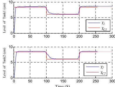
3 is used to provide the controls by minimizing equations (4) and (5) with Hp and Hc and taking into account equation (3). A first test of set point tracking can be seen in Figure 2, in which the maximum value of the iteration number for the modified DNPSO searching is set at 20 and the population size at 5. The values of Δumin and Δmax

represent the constraints for increments of u1 and u2

and they are set to equal -10V and 10V. The constraints on the controls are set at 0V and 20V.

The simulation results shown in Figures 2 and 3 illustrate that the tracking errors, despite of the variation of the set points, are always reduced with smooth control actions. This is thanks to the ability of the modified Dynamic Neighborhood PSO to minimize two objective functions while respecting the fixed values of the constraints. Furthermore, the results of the first test are quantitatively evaluated by calculating the Mean Relative Error (MRE) of the two output levels y1

and y2. The MRE are calculated by equation (21).

0 50 100 150 200 250 300

0 5 10

L

eve

l of T

ank1

(c

m

)

0 50 100 150 200 250 300

0 5 10

Time (S)

L

eve

l of T

ank2 (c

m

)

Y Y

Y Y

C2 2

[image:6.612.318.514.346.495.2]

C1 1

Figure 2: Evolution of set points and the outputs (First test)

0 50 100 150 200 250 300

0 10 20

u1

and

u2

(V

)

0 50 100 150 200 250 300

-20 0 20

Time (S)

In

cr

em

en

ts

(

V

)

u1 u2

u1 u2

 

[image:6.612.318.519.536.681.2]

1419 The MRE values of levels y1 and y2 are respectively

0.0424 and 0.0421 for a step times set at 300. The obtained values of the standard deviation (SD) of the errors outputs y1 and y2 are respectively 0.1291

and 0.0998. Taking into consideration the values of MRE and SD and the responses illustrated at Figs 2 and 3, we can note that the proposed method is capable of controlling the nonlinear MIMO system and to lead to satisfactory outputs.

 

1 ( ) ( ) ( ) 1, 2 Np Ci i Ci k i

y k y k y k

MRE i

Np









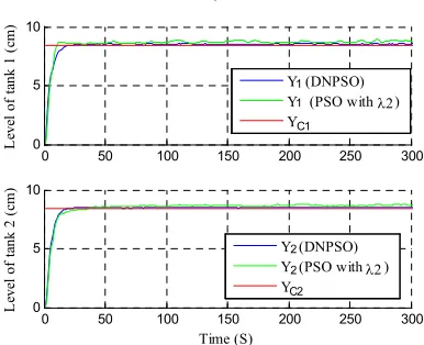
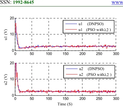
 (21)

Figures 4, 5, 6, 7, 8, 9 and Table 1 illustrate the results of the comparison between the proposed method and MPC method based on a constrained PSO algorithm with a single optimization problem defined in equation (2) with

Hp and Hc .

The values of Δumin and Δumax are set to

equal -16V and 16V. The constraints on the controls are taken at 0V and 20V. In order to avoid the effect of the randomness, the values of r1 and r2

are fixed respectively 0.1 and 0.95 for the proposed DNPSO and the PSO. Table 1 shows the MRE and the root mean square of the increments of the controls (RMSIi ) defined in equation (22).

 

2 k=1 ( ) 1, 2 Np Np i i u h RMSI i 





 (22)

In first step, the method based on modified DNPSO has been compared to the method based on PSO with the weighting factors λ1 =0.2. In this case,

the results of Figures 4, 5, 8 and Table 1 clearly indicate that the performance of two methods is very close in terms of MRE, but the performance of the method based on DNPSO is better in the term of RMSI. Then, the results shown in Figures 6, 7, 9 and Table 1 demonstrate that the performance of the method based on modified DNPSO has shown more intricate results than the one based on PSO with the weighting factors λ2=0.5 in terms of MRE

and very close in terms of RMSI.

The comparison results in term of RMSI show that the DNPSO algorithm lead to desired trajectory with small values of control increments compared to method based on PSO with fix values of the weighting factors.

This highlights the importance of the proposal method to prevent the aggressive control and to provide a progressive control law. The simulation results reported in Figure 3 illustrate the ability of the proposed method to respect of the imposed constraints.

0 50 100 150 200 250 300

0 5 10 L eve l of t ank 1 (c m)

0 50 100 150 200 250 300

0 5 10 Time (S) L eve l of t an k 2 (c m)

Y (DNPSO) Y (PSO with ) Y

[image:7.612.317.516.268.600.2]

Y (DNPSO) Y (PSO with ) Y 1 C1  1  2 2 2

Figure 4:Evolution of set points and the outputs

(comparison test with λ1)

50 100 150 200 250 300

0 10 20 u1 (V )

0 50 100 150 200 250 300

0 10 20 Time (S) u2 (V )

u1 (DNPSO) u1 (PSO with )

u2 (DNPSO) u2 (PSO with )

1

[image:7.612.321.514.449.606.2]

1

Figure 5: Evolution of the inputs (comparison test with

λ1)

0 50 100 150 200 250 300

0 5 10 L eve l of t an k 1 (c m )

0 50 100 150 200 250 300

0 5 10 Time (S) L eve l of t an k 2 (c m )

Y (DNPSO) Y (PSO with ) Y

Y (DNPSO) Y (PSO with ) Y   1 C1 C2 1 2 2

Figure 6:Evolution of set points and the outputs

(comparison test with λ2)

1420

0 50 100 150 200 250 300

0 10 20

u1

(V

)

0 50 100 150 200 250 300

0 10 20

Time (S)

u2

(V

)

u2 (DNPSO) u2 (PSO with ) u1 (DNPSO) u1 (PSO with )

[image:8.612.93.296.75.256.2]

 

Figure 7: Evolution of the inputs (comparison test with

λ2)

Therefore, the proposal method represents a compromise between the optimization of the sum quadratic of errors and the sequence of the control increments, despite sizeable computation time compared to the single objective optimization method based on PSO algorithm. However, the real-time performance of the method depends greatly on the speed of the proposed algorithm. So, it is important to improve the convergence time in order to apply the developed strategy to other classes of faster nonlinear systems. In this context, it is important to formulate stopping conditions allowing the algorithm to find optimal solutions while respecting the sampling period. In other words it is necessary to improve the performance of the algorithm in terms of convergence and speed.

6. CONCLUSION

This paper has described a new kind of Multivariable Multi-Objective Predictive Control using a modified Dynamic Neighborhood PSO algorithm and the T-S fuzzy modeling approach. This strategy has been applied to control the Quadruple-Tank process.

TABLE 1:COMPARISON RESULTS. DNPSO

method Single objective based on PSO

λ1 λ2

MRE1 0.0330 0.0588 0.0822

MRE2 0.0296 0.0528 0.0645

RMSI1 0.8571 1.3923 0.7668

RMSI2 0.8841 1.1606 0.8497

Computation time (s)

0.61 0.53

0 50 100 150 200 250 300

-10 0 10 20

In

cr

em

en

ts

o

f

u1

(

V

)

0 50 100 150 200 250 300

-10 0 10 20

Time (S)

In

cr

em

en

ts

o

f

u2

(

V)

u1 (DNPSO) u1 (PSO with )

u2 (DNPSO) u2 (PSO with )

 



 

[image:8.612.318.514.99.445.2]



Figure. 8: The increments of the controls (comparison test with λ1 )

0 50 100 150 200 250 300

-10 0 10 20

In

cr

em

en

ts

o

f

u1

(

V

)

0 50 100 150 200 250 300

-10 0 10 20

Time (S)

In

cr

em

en

ts

o

f

u2

(

V)

u1 (DNPSO) u1 (PSO with )

u2 (DNPSO) u2 (PSO with )



 



 

 

Figure 9: The increments of the controls (comparison test with λ2 )

[image:8.612.96.295.584.698.2]

1421 REFRENCES:

[1] Ellis M. and Christofides P. D., "Integrating dynamic economic optimization and model predictive control for optimal operation of nonlinear process systems," Control Engineering Practice, vol. 22, 2014, pp. 242-251.

[2] Nery Júnior G. A., Martins M. A. F., and Kalid R., "A PSO-based optimal tuning strategy for constrained multivariable predictive controllers with model uncertainty," ISA Transactions, vol. 53, No. 2, 2014, pp. 560-567.

[3] Thamallah A., Sakly A., and M’Sahli F.,“Constrained multivariable predictive controller based on PSO algorithm and T-S fuzzy modeling approach”, in 15th International Conference on Sciences and Techniques of Automatic Control and Computer Engineering (STA), 2014, pp. 117-122.

[4] Mc Namara P., Negenborn R. R., De Schutter B., and Lightbody G., "Weight optimisation for iterative distributed model predictive control applied to power networks," Engineering Applications of Artificial Intelligence, vol. 26, No. 1, 2013, pp. 532-543.

[5] Khouaja A., Garna T., Ragot J., and Messaoud H., "Nonlinear predictive controller based on S-PARAFAC Volterra models applied to a communicating two-tank system," International Journal of Control, vol. 88, No. 8, 2015, pp. 1456-1471.

[6] Laabidi K., Bouani F., and Ksouri M., "Multi-criteria optimization in nonlinear predictive control," Mathematics and Computers in Simulation, vol. 76, No. 5–6, 2008, pp. 363-374.

[7] Ben Aicha F., Bouani F., and Ksouri M., "A multivariable multiobjective predictive controller," International Journal of Applied Mathematics and Computer Science, vol. 23, No. 1, 2013, p. 35.

[8] García C. E., Prett D. M., and Morari M., "Model predictive control: Theory and practice—A survey," Automatica, vol. 25, No. 3, 1989, pp. 335-348.

[9] Clarke D. W., Mohtadi C., and Tuffs P. S., "Generalized predictive control—Part I. The basic algorithm," Automatica, vol. 23, No. 2, 1987, pp. 137-148.

[10] Clarke D. W. and Mohtadi C., "Properties of generalized predictive control," Automatica, vol. 25, No. 6, 1989, pp. 859-875.

[11] Reyes-Sierra M. and Coello C. A. C., "Multi-Objective Particle Swarm Optimizers: A Survey of the State-of-the-Art," International Journal of Computational Intelligence Research, vol. 2, No. 3, 2006, pp. 287–308.

[12] Salehpour M. and TABAN M. R., "Two approaches on carrier frequency offset estimation in MIMO OFDM systems," Iranian Journal of Science and Technology Transactions of Electrical Engineering, vol. 38, No. E2, 2014, pp. 123-136.

[13] Bahareh Nakisa, Mohammad Naim Rastgoo, Mohammad Faidzul Nasrudin, and Nazri M. Z. A., "A multi-swarm particle swarm optimization with local search on multi-robot search system," Journal of Theoretical and Applied Information Technology, vol. 71 No. 1, 2015, pp. 129-136.

[14] BenNasr N., "Contributions à l’Analyse et la Synthèse de la Commande Prédictive des Systèmes Non Linéaires," Ecole Nationale d’Ingénieurs de Sfax, Tunisie, 2007.

[15] "TWO APPROACHES ON CARRIER FREQUENCY OFFSET ESTIMATION IN MIMO OFDM SYSTEMS," Iranian Journal of Science and Technology Transactions of Electrical Engineering, vol. 38, No. E2, 2014, pp. 123-136.

[16] Johansen T. A. and Hunt K. J.,“A computational approach to approximate input/state feedback linearization”, in Proceedings of the 39th IEEE Conference on Decision and Control (Cat. No.00CH37187), 2000, pp. 4467-4472 vol.5.

[17] Jiang H., Kwong C. K., Chen Z., and Ysim Y. C., "Chaos particle swarm optimization and T–S fuzzy modeling approaches to constrained predictive control," Expert Systems with Applications, vol. 39, No. 1, 2012, pp. 194-201.

[18] Ogata K., "Fluid Systems and Thermal Systems," in System Dynamics, K. Ogata, Ed., fourth ed New Jersey, USA: Pearson Prentice Hall, 2004.

[19] Chadli M. and Borne P., "Multiple Model Representation," in Multiple Models Approach in Automation: Takagi-Sugeno Fuzzy Systems, B. Dubuisson, Ed., First ed Great Britain and the United States: Wiley-ISTE, 2012.

1422 [21] Ben Abdennour R., Ksouri M., and Favier G.,

"Application of Fuzzy Logic to the On-Line Adjustment of the Parameters of a Generalized Predictive Controller," Intelligent Automation & Soft Computing, vol. 4, No. 3, 1998, pp. 197-213.

[22] Xiaohui H. and Eberhart R.,“Multiobjective optimization using dynamic neighborhood particle swarm optimization”, in Evolutionary Computation, 2002. CEC '02. Proceedings of the 2002 Congress on, 2002, pp. 1677-1681. [23] Takagi T. and Sugeno M., "Fuzzy identification

of systems and its applications to modeling and control," IEEE Transactions on Systems, Man, and Cybernetics, vol. SMC-15, No. 1, 1985, pp. 116-132.

[24] Johansson K. H., "The quadruple-tank process: a multivariable laboratory process with an adjustable zero," IEEE Transactions on Control Systems Technology, vol. 8, No. 3, 2000, pp. 456-465.