A Magnetic Field Integral Equation Based Iterative Solver
for Scattered Field Prediction
Robert Brem* and Thomas F. Eibert
Abstract—An iterative solution scheme based on the magnetic field integral equation (MFIE) to compute electromagnetic scattering for arbitrary, perfect electrically conducting (PEC) objects is topic of this contribution. The method uses simple and efficient approaches for the computation of surface current interactions which are typically found in the well-known iterative physical optics (IPO) technique. However, the proposed method is not asymptotic, since no physical optics (PO) concepts are utilized. Furthermore, a least squares correction method is introduced, which is applied not on the complete current vector, but on individual groups of currents. This helps to quickly reduce the residual error and to improve convergence. The result is a simple method which is capable to improve the simulation results obtained by pure asymptotic methods such as PO or shooting and bouncing rays (SBR). The method can be regarded as a simplified iterative method of moments (MoM) technique. Numerical examples show that the proposed approach is advantageous e.g., in problem cases where the neglect of diffraction effects or currents in shadow regions would cause large errors. It also provides an improved prediction of the peak scattering contributions.
1. INTRODUCTION
Although the high-frequency approximation methods PO or SBR provide excellent field predictions for large object scattering in many applications, problem cases exist where these simple methods fail to provide reliable results. Effects such as strong multiple scattering, complicated diffraction mechanisms or significant scattering contributions of currents in shadow regions are difficult to be taken into account accurately. If improved accuracy is desired and exact methods such as MoM are computationally too expensive, hybrid methods are appropriate alternatives. Much research effort has been invested in the development of such efficient numerical techniques, which combine exact and approximate (asymptotic) methods in order to reduce the computational cost. Typically, complex parts of a scattering or radiating object are treated by MoM or, e.g., a finite element (FE) method, whereas large, smooth parts are treated by ray- or current-based asymptotic approaches. The interaction between the currents in these separately computed domains has to be taken into account accurately. This is normally done in an iterative manner. Well-known examples are the PO-MoM approach [1], which can be improved by incorporating higher-order edge or surface diffraction effects [2, 3]. Other methods employ electric and magnetic field integral equation (EFIE-MFIE) formulations to different domains, where the MFIE is iteratively approximated by PO [4] or use sophisticated iterative techniques with special basis functions in the hybrid PO-MoM approach [5]. A ray-based geometrical theory of diffraction (GTD)-MoM technique is introduced in [6]. Advanced methods also use the uniform theory of diffraction (UTD) in combination with FE and MoM [7].
Iterative methods based on a repeated evaluation of the MFIE follow a different concept to lower the computational cost compared to MoM. Here, the introduction of separate domains is not required.
Received 25 July 2014, Accepted 25 November 2014, Scheduled 4 December 2014
* Corresponding author: Robert Brem ([email protected]).
Examples are the methods proposed in [8, 9] which are applied to simple scattering objects. A similar method is the IPO, which was developed to compute the scattering from cavities [10, 11]. It is also based on an iterative computation of the MFIE, starting with an initial current vector obtained by PO. The computed currents of one iteration step are the new radiating currents in the next step. The computation is repeated until a certain accuracy is reached (a residual error of about 0.1 is typically acceptable and accurate enough for practical radar cross section (RCS) cavity problems).
The proposed method in this paper is based on an iterative solution of the MFIE, applicable to arbitrary 3D PEC scattering objects. The interaction between currents is computed in the same efficient manner (low sampling point density and fast far-field approximation (FaFFA) [12]) as with IPO. The MFIE is, however, exactly evaluated, i.e., no asymptotic concepts are applied. A correction method to improve the convergence of the iterative scheme, which directly uses the group partitioning introduced by the FaFFA, is applied. For all groups (boxes) a correction factor is computed and multiplied with all corresponding box currents. The factors are determined by solving a linear least squares problem so that the MFIE for all boxes is fulfilled with minimum quadratic error. In Section 2 the evaluation of the MFIE is shown and in Section 3 the correction method is introduced. This is followed by a demonstration of the performance with numerical examples and a conclusion.
2. ITERATIVE SOLUTION OF THE MFIE AND ITS IMPLEMENTATION
The magnetic field integral equation for the PEC case is given as [13]
J(r) = 2ˆn(r)×Hi(r) + 2ˆn(r)× −
SJ
r× ∇Gr,rdS, (1)
where J(r) is the electric surface current density on the surface S of the scattering body, ˆn(r) the outward pointing unit normal vector, and Hi(r) the incident magnetic field. The bar at the integral sign stands for the principal value integral with points r=r excluded from integration. The gradient of the Green’s function is
∇Gr,r= e
−jkR
4πR3
1 +jkRR, (2)
whereR =|R|=|r−r|. The integral
˜
Hs(r) =−
SJ
r× ∇G(r,r)dS (3)
accounts for the radiation of the surface currents. With the boundary conditionJ= ˆn×(Hi+Hs) on
S, the relation
Hs(r) =Hi(r) + 2 ˜Hs(r) (4)
holds between the scattered magnetic field and the sum of the incident magnetic field and the field produced by the integral.
A triangle mesh with a total number of NP patches is used for surface modeling. The surface current density Jk on triangle k(k= 1, . . . , NP), is expressed by two orthogonal tangential vectors of this triangle, weighted by corresponding current density coefficientsIk,1/2. These have to be determined
within the iterative solution scheme:
Jk(r) =
Ik,1tˆk,1+Ik,2ˆtk,2 forrin triangle k
0 otherwise. (5)
This pulse basis function approach is similar to the simplest form in [14]. The current locations are assumed to be at the centroidsrk of the triangles which are also the locations of the observation points for the evaluation of the integral in (3). In contrast to the traditional MoM-approach with Rao-Wilton-Glisson (RWG) functions, this point based description of currents is ideally suited for the MFIE [14].
Box i Box j
currents
Box i Box j
currents currents currents
(a) (b)
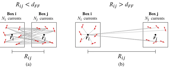
Figure 1. Computation of box interactionj→i. (a) Near-field case and (b) far-field case with FaFFA acceleration.
D is the side length of a box. The interaction of currents in far-field box pairs is done in a two-step scheme. First, the field contributions of all currents in the source box are computed at the center of the observation box, then, the contributions for all currents in the observation box are evaluated by applying a location dependent phase shift on the center field. This far-field computation has a linear complexity and the total complexity of FaFFA will be O(N1.5) with an optimally chosen number of currents per box (=√N).
In order to generate the box structure in the proposed algorithm, first the maximum extension of the scattering object in x-, y- and z-direction is determined. Then, this space is subdivided into cubic boxes where empty boxes are neglected. All boxes have an identical side length, which can be arbitrarily specified. The possibility to adjust this value is useful for the applied correction scheme presented in Section 3. The assignment of currents to boxes is directly given by this regular 3D grid structure. For the numerical examples shown later, the box size is chosen on the order of a few wavelengths, which is smaller than the optimal value so that the complexity of the interaction computation will lie betweenO(N1.5). . .O(N2). Nevertheless, due to the utilized simple MFIE evaluation, fast simulations are possible. This issue will be further discussed in Section 3.
The current densities in observation box i are denoted with index m (m = 1, . . . , Ni) and the current densities in source boxj with index n(n= 1, . . . , Nj). The total number of boxes isNB and the centers of the boxes are denoted byriandrj, respectively. The current densities induced by incident and radiated fields on trianglekare obtained by taking the scalar product of a tangential vector on this triangle with the first or the second term of the RHS of (1), i.e.,
Ik,i 1/2 = ˆtk,1/2·
2ˆnk×Hi(rk) I˜k,s1/2= ˆtk,1/2·
2ˆnk×H˜s(rk) , (6)
where ˆtk,1/2 are the tangential vectors and ˆnk the normal vector of triangle k. By grouping all current
densities Ik,i 1/2 in vector Iii and all current densities ˜Ik,s1/2 in vector ˜Isi, the current density vector Ii of
boxican be written as
Ii =Iii+ ˜Isi =Iii+ NB
j=1
˜
Isij, (7)
where ˜Isij is the induced surface current density vector in boxicaused by box j. For the near-field case, the induced current densities (ˆtm,1- or ˆtm,2-component) on patch m in box iby the contribution of all
current densities n= 1, . . . , Nj in box j are computed as
˜Is
mj,1/2 = ˆtm,1/2·
⎡ ⎣2ˆnm×
Nj
n=1
ΔAn Q
q=1
Jn×Rmn,qe
−jkRmn,q
4πR3
mn,q (1 +jkRmn,q)wq ⎤ ⎦
= ˆtm,1/2·
⎡
⎣2ˆnm×Nj n=1
ΔAn Q
q=1
In,1ˆtn,1×Rmn,q+In,2ˆtn,2×Rmn,q
Kmn,qwq
⎤
where Kmn,q is the complex term exp(−jkRmn,q)(1 +jkRmn,q)/(4πRmn,q), ΔAn is the corresponding triangle area, Rmn,q is the vector from quadrature pointq (q= 1, . . . , Q) on triangle nto the centroid of triangle m, i.e., Rmn,q =rm−rn,q and wq is the weight for numerical integration. The application of a quadrature rule with Q >1 is useful for nearby patches and improves the accuracy of the integral evaluation. All current densities ˜Ismj,1/2 (m= 1, . . . , Ni) together form the complex 2Ni×1 vector ˜Isij, where 2Ni is due to both tangential vectors. By introducing the interaction matrixAij and the current density vector Ij, formed by all current densities In,1/2 of boxj, the compact representation
˜Is
ij =AijIj Aij ∈C2Ni×2Nj (9)
can be given. Therefore, 4NiNj operations are required for evaluation of the matrix-vector product to compute a surface current density vector ˜Isij in the near-field case. For the far-field case, first, the scattered field contribution of all current densities in boxj at the box center ri of box iis computed as
˜
Hsij = Nj
n=1
ΔAn Q
q=1
Jn×Rin,qe
−jkRin,q
4πR3
in,q
(1 +jkRin,q)wq
= Nj
n=1
ΔAn Q
q=1
In,1tˆn,1×Rin,q+In,2ˆtn,2×Rin,q
Kin,qwq, (10)
whereKin,q = exp(−jkRin,q)(1 +jkRin,q)/(4πRin,q3 ),Rin,q =ri−rn,q and ˜Hsij is a complex 3D vector. In compact form, this can be written as
˜
Hsij =AijIj Aij ∈C3×2Nj, (11) where the matrix Aij directly describes the mapping of a current density vector with complex scalar elements on a three-dimensional complex vector in space. In the next step, the induced current densities on the Ni patches can be obtained by applying a phase shift and the vector operation according to
˜
Ismj,1/2= ˆtm,1/2·
2ˆnm×H˜sij e−jk
ˆ
Rij·(rm−ri)
. (12)
Similar to the near-field case, all current densities ˜Ismj,1/2 together build the current density vector ˜Isij. The number of operations in the far-field case is 2Ni+ 6Nj.
With the precomputed interaction matricesAij for all near- and far-field cases, the MFIE according to (1) is iteratively evaluated. The start vector J(0) is given by a PO computation. In contrast to the classical IPO, shadowed parts of the scattering body are also excited by Hi and the radiated fields of new currents, i.e., interactions between currents are completely taken into account. The proposed method is therefore not based on the asymptotic PO approximation, it is an iterative MoM approach.
3. CORRECTION METHOD
In general, convergence of the iterative MFIE computation cannot be guaranteed so that an appropriate handling of this problem is required. If (1) is written in matrix-vector form, the given system matrix is required to have a spectral radius smaller than one to ensure a convergent solution. In order to stabilize the computation, a relaxation parameter can be introduced or even a technique such as the generalized minimal residual method (GMRES) could be applied. A simplified GMRES approach for cavity problems is introduced in [11]. However, as stated in [15], these methods typically show a very slow convergence due to the introduced approximations. It is a good alternative to use simpler correction methods, monitor the residual error in each iteration step and stop the procedure when a certain accuracy is reached. In this spirit works our proposed correction method.
The obtained total current distribution on the scatterer at an iteration stepl (l= 1, . . . , Nit with
Nit being the total number of iterations) can be written similar to (1) as
J(l)= 2ˆn×Hi+ 2ˆn× −
SJ
(l−1)× ∇
The current densityJ(1) is computed via the initial current density vectorJ(0), which is obtained by PO approximation. Similar to the presentation in (7), the complete current density vector can be written as
I(l)=Ii+ ˜Is(l−1). (14)
The optimal current density found at step lwould perfectly satisfy the MFIE, i.e., pluggingJ(l)instead of J(l−1) into the integral of (13) or replacing ˜Is(l−1) by ˜Is(l) in (14), respectively, would exactly fulfill these equations. However, in reality an error remains, which can be expressed as
ΔJ(l)=J(l)−2ˆn×Hi−2ˆn× −
SJ
(l)× ∇G dS =J(l)−J(l+1), (15)
or according to (14) as
ΔI(l)=I(l)−Ii−˜Is(l)=I(l)−I(l+1). (16)
The corresponding residual error can thus be defined by
R(l) =
I(l)−˜Is(l)−Ii
Ii . (17)
The errorR(l) is related to the current density vector ˜Is(l), which is computed in the stepl+ 1 (s. (14)), i.e., the residual errorR(l) is also computed in this step. In other words, the step of the residual error is always related to the step of the current densities which are plugged into the MFIE for error evaluation according to (15) or (16). In step l+ 2 the error R(l+1) is obtained and compared with R(l). If the error decreases, i.e.,R(l+1) < R(l), nothing changes (the computed current densityI(l+1) is used for step
l+ 2 to obtainI(l+2) as already done), otherwise, a complex correction factor is computed for each box, i.e., all current densities of a box at step l+ 1 are equally weighted and a new current density I(l+2) is generated. The correction factors αi (i= 1, . . . , NB) are determined in such a way that the MFIE for each boxiis most accurately fulfilled, i.e., the equation
αiI(il)− NB
j=1
αj˜Isij(l)=Iii (18)
should hold. This is enforced by solving a linear least squares problem. (18) can be written as
α1
˜
Is11(l)−I(1l)
+α2˜Is12(l)+α3˜Is13(l)+. . .+αNB˜Is
(l)
1NB =−Ii1
α1˜Is21(l)+α2
˜
Is22(l)−I(2l)
+α3˜I23s(l)+. . .+αNB˜Is
(l)
2NB =−Ii2
α1˜Is31(l)+α2˜Is32(l)+α3
˜
Is33(l)−I(3l)
+. . .+αNB˜Is
(l)
3NB =−Ii3
.. .
α1˜IsN(Bl)1+α2˜INs(Bl)2+α3˜INs(lB)3+. . .+αNB
˜Is(l)
NBNB −I
(l)
NB
=−IiNB.
(19)
In matrix form this can be expressed as
Mα=b (20)
with M ∈ C2N×NB, α ∈ CNB×1 and b ∈ C2N×1. The vector α of this overdetermined system is
computed by solving the least squares problem
min
α Mα−b 2
, (21)
where the LAPACK routinecgels, using a QR factorization ofM, is utilized. The complexity of this correction is proportional toN N2
B. Since NB can be seen as dependent on
with the simple MFIE evaluation and the application of only a few iterations (and therefore possible correction steps), fast simulations are possible. This can be further improved by a similarly efficient hierarchical implementation as in the MLFMM with aggregation, translation and disaggregation steps. The group-wise improvement of the current densities can help to quickly reduce the residual error. Stability problems may be avoided by simply choosing a smaller box size, so that more correction coefficients αi are introduced. However, it is important to note that such a scheme can not guarantee stability. For critical cases which do not show convergence to the desired degree, even for a large number of correction coefficients, a finer current sampling density should be applied, i.e., more currents should be introduced to model the surface current distribution with better accuracy. The method can be further extended to weight the two orthogonal current density components on a triangle patch individually for each box, so that 2NB coefficients are introduced. In this case (18) can be written as
αi,1I(i,l1)
αi,2I(i,l2)
−
NB
j=1 Aij
αj,1I(j,l)1
αj,2I(j,l)2
=Iii. (22)
The coefficient αi,1 is multiplied with all ˆt1-current density components of box i and αi,2 with all
ˆ
t2-current density components of boxi.
4. NUMERICAL EXAMPLES
The following examples show the performance of the iterative solver, denoted as iterative MFIE (IMFIE). A comparison between MoM, SBR, IPO and IMFIE concerning achieved accuracies and required simulation times is performed. In order to obtain the MoM reference solutions, CST Microwave Studio [16] was used, where the residual error to achieve was set to 10−3. For SBR, IPO and IMFIE own codes are applied. All simulations are performed on a system with 12×3.47 GHz computing power. In order to provide a reasonable comparison to our single-threaded test codes, the thread use in CST is set to 1.
4.1. Cube
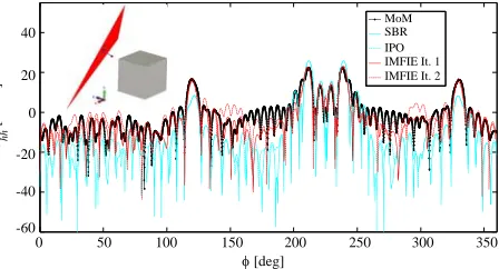
The bistatic RCS for scattering at a PEC cube with a side length of 10 wavelengths and plane wave incidence is shown for the different computational techniques MoM, SBR, IPO and IMFIE according to Fig. 2. SBR and IPO give (almost exactly) the same results, which are obviously very inaccurate. Both methods fail to give a good RCS prediction since diffraction contributions are completely neglected. The IPO solution is constant, it does not improve with more iterations since no multiple bounces occur. Only after one iteration, the IMFIE scheme computes an RCS close to the MoM solution, where the agreement is very good in the main scattering directions. A mesh discretization of λ/3 (mean triangle edge length) and a box side length of 1λare chosen. Table 1 compares simulation times (with all solvers utilizing 1 thread) and accuracies of the methods.
Due to the very simple MFIE evaluation and the coarse current density, it is clear that the IMFIE solution does not perfectly match the MoM results of CST Microwave Studio. This is also observed in
40
20
0
-40 -20
-60
σ
[dBsw]
hh
0 50 100 150 200 250 300 350
φ [deg]
MoM SBR IPO IMFIE It. 1 IMFIE It. 2
Figure 2. Bistatic RCS (hh) for a 1 m×1 m×1 m PEC cube for plane wave incidence with φ= 45◦,
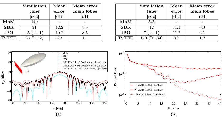
Table 1. Comparison of simulation results for the cube.
Simulation time [sec]
Mean error [dB]
Mean error main lobes
[dB]
MoM 149 -
-SBR 21 12.2 3.5
IPO 65 (It. 1) 10.2 3.5 IMFIE 85 (It. 2) 5.3 1.1
Table 2. Comparison of simulation results for the NASA Almond.
Simulation time [sec]
Mean error [dB]
Mean error main lobes
[dB]
MoM 545 -
-SBR 12 11.3 6.0
IPO 7 (It. 1) 11.2 6.1 IMFIE 170 (It. 39) 3.7 1.2
40
20
0
-40 -20 60
σ
[dBsw]
hh
0 50 100 150 200 250 300 350
φ [deg]
10
10 10
Residual Error
0
-1
-2
0 5 10 15 20 25 30 35 40
Iteration
(a) (b)
MoM SBR IPO
IMFIE It. 34 (16 Coefficients, 1 per box) IMFIE It. 23 (98 Coefficients, 1 per box) IMFIE It. 39 (196 Coefficients, 2 per box)
16 Coefficients (1 per box) 98 Coefficients (1 per box) 196 Coefficients (2 per box)
Figure 3. Simulation of a 9.936 in long PEC NASA Almond for plane wave incidence with φ = 0◦,
θ= 90◦,f = 7 GHz. Observation range φ= 0◦, . . . , 360◦,θ= 90◦. (a) Bistatic RCS (hh). (b) Residual error.
the following examples. One might expect a good agreement of the IMFIE results with MoM for all observation angles. However, larger deviations can occur for observations with low RCS due to some inaccuracies in the currents. Nevertheless, the average RCS level for these observations is typically better predicted than with asymptotic methods. For the desired goal — the efficient improvement of simple asymptotic solver results in problematic cases — this method is very well suited.
4.2. NASA Almond
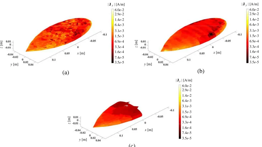
The bistatic RCS result of a PEC NASA Almond benchmark target [17] is shown in Fig. 3(a). The IMFIE results are shown for different numbers of correction coefficients, where the results with lowest residual error, see Fig. 3(b), are plotted. For the chosen discretization and the second case with 98 coefficients, the solution starts to diverge after 23 iterations. Increasing the number of coefficients improves the convergence significantly. The IMFIE computed RCS is in much better agreement with MoM (mean error 3.7 dB with 196 coefficients) than the SBR and IPO results (mean error approx. 11 dB). A mesh discretization of λ/4 and a box side length of λ/2 are chosen for IPO and IMFIE. Fig. 4(a), Fig. 4(b) and Fig. 4(c) show the surface current densities (magnitude of Jy-component) for MoM, IMFIE and SBR method, respectively. The IPO result is more or less similar to the SBR result. Table 2 shows the simulation data.
4.3. Glider
(a) (b) 6.0e-2 2.9e-2 1.4e-2 6.4e-3 3.1e-3 1.5e-3 6.9e-4 3.3e-4 1.6e-4 7.4e-5 3.5e-5 6.0e-2 2.9e-2 1.4e-2 6.4e-3 3.1e-3 1.5e-3 6.9e-4 3.3e-4 1.6e-4 7.4e-5 3.5e-5
| J | [A/m]y
6.0e-2 2.9e-2 1.4e-2 6.4e-3 3.1e-3 1.5e-3 6.9e-4 3.3e-4 1.6e-4 7.4e-5 3.5e-5 (c) y [m] x [m] y [m] x [m] y [m] x [m] z [m] z [m] z [m]
Figure 4. Surface current distributions (magnitude ofJy-component) on the PEC NASA Almond for plane wave incidence with φ= 0◦,θ= 90◦,f = 7 GHz. (a) MoM. (b) IMFIE (It. 39). (c) SBR.
φ [deg]
220 230 240 250 260 270 280 290 300 310 320
MoM SBR IPO It. 3 IMFIE It. 3 40 20 0 -20 -10 50 σ [dBsw] hh 30 10
Figure 5. Bistatic RCS (hh) for a 14.5 m long, 14 m wide PEC glider for plane wave incidence with
φ= 270◦,θ= 135◦,f = 1 GHz. Observation range φ= 220◦, . . . , 320◦,θ= 90◦.
Table 3. Comparison of simulation results for the glider.
Simulation time [sec]
Mean error [dB]
Mean error main lobes [dB]
MoM 1712 -
-SBR 95 8.2 2.3
IPO 768 (It. 3) 7.9 1.3
IMFIE 1680 (It. 3) 8.4 1.3
5. CONCLUSION
solvers with complicated diffraction methods. As numerical examples revealed, an accurate scattered field prediction can be achieved with only a few MFIE iterations. Problem cases, where simple physical optics (PO) or shooting and bouncing rays (SBR) computations provide only poor results, can be properly treated. A precise determination of RCS peak values is an important advantage. A hierarchical interaction computation similar to the multilevel fast multipole method (MLFMM) scheme is recommended for large simulation tasks to further improve the efficiency.
REFERENCES
1. Jakobus, U. and F. Landstorfer, “Improved PO-MM hybrid formulation for scattering from three-dimensional perfectly conducting bodies of arbitrary shape,” IEEE Trans. Antennas Propagat., Vol. 43, No. 2, 162–169, 1995.
2. Jakobus, U. and F. Landstorfer, “Improvement of the PO-MoM hybrid method by accounting for effects of perfectly conducting wedges,” IEEE Trans. Antennas Propagat., Vol. 43, No. 10, 1123– 1129, 1995.
3. Jakobus, U. and F. Landstorfer, “Application of Fock currents for curved convex surfaces within the framework of a current-based hybrid method,”Third International Conference on Computation in Electromagnetics, 415–420, Bath, UK, Apr. 1996.
4. Hodges, R. and Y. Rahmat-Samii, “An iterative current-based hybrid method for complex structures,”IEEE Trans. Antennas Propagat., Vol. 45, No. 2, 265–276, 1997.
5. Tasic, M. and B. Kolundzija, “Efficient analysis of large scatterers by physical optics driven method of moments,” IEEE Trans. Antennas Propagat., Vol. 59, No. 8, 2905–2915, 2011.
6. Thiele, G. and T. Newhouse, “A hybrid technique for combining moment methods with the geometrical theory of diffraction,” IEEE Trans. Antennas Propagat., Vol. 23, No. 1, 62–69, 1975. 7. Tzoulis, A. and T. Eibert, “A hybrid FEBI-MLFMM-UTD method for numerical solutions of
electromagnetic problems including arbitrarily shaped and electrically large objects,”IEEE Trans. Antennas Propagat., Vol. 53, No. 10, 3358–3366, 2005.
8. Kaye, M., P. Murthy, and G. Thiele, “An iterative method for solving scattering problems,” IEEE Trans. Antennas Propagat., Vol. 33, No. 11, 1272–1279, 1985.
9. Murthy, P., K. Hill, and G. Thiele, “A hybrid-iterative method for scattering problems,” IEEE Trans. Antennas Propagat., Vol. 34, No. 10, 1173–1180, 1986.
10. Obelleiro, F., J. Rodriguez, and R. Burkholder, “An iterative physical optics approach for analyzing the electromagnetic scattering by large open-ended cavities,” IEEE Trans. Antennas Propagat., Vol. 43, No. 4, 356–361, 1995.
11. Burkholder, R., “A fast and rapidly convergent iterative physical optics algorithm for computing the RCS of open-ended cavities,” Appl. Computational Electromagn. Soc. J., Vol. 16, No. 1, 53–60, 2001.
12. Lu, C. and W. Chew, “Fast far-field approximation for calculating the RCS of large objects,”
Microwave Opt. Tech. Letters, Vol. 8, No. 5, 238–241, 1995.
13. Gibson, W., The Method of Moments in Electromagnetics, Chapman & Hall/CRC, Boca Raton, 2008.
14. Kang, G., J. Song, W. Chew, K. Donepudi, and J. Jin, “A novel grid-robust higher order vector basis function for the method of moments,” IEEE Trans. Antennas Propagat., Vol. 49, No. 6, 908–915, 2001.
15. Burkholder, R. and T. Lundin, “Forward-backward iterative physical optics algorithm for computing the RCS of open-ended cavities,” IEEE Trans. Antennas Propagat., Vol. 53, No. 2, 793–799, 2005.
16. https://www.cst.com/Products/CSTMWS.