Scholarship@Western
Scholarship@Western
Electronic Thesis and Dissertation Repository
8-26-2016 12:00 AM
A Sequence of Symmetric Bézout Matrix Polynomials
A Sequence of Symmetric Bézout Matrix Polynomials
Leili Rafiee Sevyeri
The University of Western Ontario Supervisor
Rob Corless
The University of Western Ontario
Graduate Program in Applied Mathematics
A thesis submitted in partial fulfillment of the requirements for the degree in Master of Science © Leili Rafiee Sevyeri 2016
Follow this and additional works at: https://ir.lib.uwo.ca/etd
Recommended Citation Recommended Citation
Rafiee Sevyeri, Leili, "A Sequence of Symmetric Bézout Matrix Polynomials" (2016). Electronic Thesis and Dissertation Repository. 4083.
https://ir.lib.uwo.ca/etd/4083
This Dissertation/Thesis is brought to you for free and open access by Scholarship@Western. It has been accepted for inclusion in Electronic Thesis and Dissertation Repository by an authorized administrator of
Abstract
There are problems concerning the set of root of a sequence of polynomials. A simple question
is to ask if the set of roots lies entirely in real numbers. Many approaches to answering this
question are known. The main object of this dissertation is to develop new tools for tackling the
above problem. In order to be able to apply the ideas we define a specific numerical sequence,
and then we consider the sequence of their minimal polynomials over the rational numbers.
The first step is to find a recursive way of defining the sequence of polynomials by using
the so-called B´ezout matrices, which are a specific family of matrix polynomials. Having the
construction of minimal polynomials as the determinant of some B´ezout matrix, we interpret
the roots of each polynomial as eigenvalues of the corresponding B´ezout matrix. Then by using
a symmetric linearization of such matrix polynomial we can talk about the real roots.
Keywords: Matrix Polynomials, Linearization, B´ezout Matrix.
First and foremost my deepest gratitude is to my advisor, Prof. Rob Corless. I have been amazingly fortunate to have an advisor who has supported me throughout my thesis with his
motivation, enthusiasm, and immense knowledge. His patience and support helped me
over-come many crisis situations and finish this dissertation. The door to Rob’s office was always
open whenever I ran into a trouble spot or had a question about my research or writing. One
simply could not wish for a better or friendlier supervisor. I hope that one day I would become
as good an advisor to my students as Rob has been to me.
Besides my advisor, I would like to thank Prof. David Jeffery for his constant positive
at-titude and for all the encouragements he gave throughout the process. I am proud, honoured
and extremely grateful to have been able to work with such amazingly talented researchers, but
most of all, who are also extremely kind human beings.Rob,David.
For having the opportunity to study in the Western University, I want to huge thank Prof.Lindi
Wahlto introduce me to Rob and helped me make a right decision early at the beginning of
my Master program.
This thesis would have never been possible without my loving husband,Armin. Words would
never say how grateful I am to you. I am truly appreciative of all you have done for me over
the years. I could not have reached my goals without your help and support. You really gave
me the reason to continue. You have made me feel special even when times were tough for
me. You have been my pillar of strength through all my ups and downs. I feel blessed to be a
part of your life, and am fortunate to be married to the most kind-hearted and generous person
I have ever known. I love you more and more everyday. You can take all the credit for much
of what I have achieved and what I will achieve in the future.
Finally, I acknowledge the people who mean a lot to me, my parents, Maman and Baba,
for showing faith in me and giving me liberty to choose what I desired. I salute you all for the
selfless love, care, pain and sacrifice you did to shape my life. Although you hardly understood
what I researched on, you were willing to support any decision I made. I would never be able
to pay back the love and affection showered upon by my parents. Also I express my thanks
to my sistersLaya andSara, for their support, valuable prayers, their selfless love, care and
dedicated efforts which contributed a lot for completion of my thesis. Even though we are
thousand of miles away, you were always there whenever I needed you.
My heart felt regard goes to my parents in law, bothers in law, Arash and Aryo for their
love and moral support.
Thank you,Allah, for always being there for me. This thesis is only a beginning of my journey.
Abstract i
Acknowledgement ii
List of Figures vi
List of Tables vii
List of Appendices viii
1 Introduction 1
2 Preliminaries 8
2.1 Basic Definitions . . . 8
2.2 Minimal Polynomials and Algebraic Extensions . . . 10
2.3 Roots of Polynomials . . . 15
2.4 Solving Bivariate Polynomials . . . 16
3 Matrix Polynomials 22 3.1 Basic Definition . . . 22
3.1.1 Matrix Polynomial . . . 22
3.1.2 Generalized Eigenvalues and Eigenvalue Problem . . . 24
3.1.3 The Companion Pencil . . . 25
3.2 B´ezout Matrix . . . 27
3.3 B´ezout Matrix in Lagrange Basis . . . 29
3.4 Linearization of a Matrix polynomial . . . 33
3.5 Linearization with Lagrange Basis . . . 38
4 A Sequence of Symmetric B´ezout Matrix Polynomials 40
4.1 Introduction . . . 40
4.2 {ui}is Algebraic over the set of Rational Numbers . . . 41
4.3 Boundary of{ui} . . . 42
4.4 Minimal Polynomials of{ui} . . . 44
4.5 Roots of Minimal Polynomials . . . 47
4.6 Symmetric Linearization of the B´ezout Matrix . . . 50
5 Concluding Remarks 54 5.1 Future Work . . . 54
5.1.1 Largest Root of{pi} . . . 54
5.1.2 Distribution of Zeros of{pi} . . . 55
5.1.3 Recursion Between B´ezout Matrices . . . 55
Bibliography 55
Curriculum Vitae 61
1.1 Cylindrical bucket with a drainage hole . . . 2
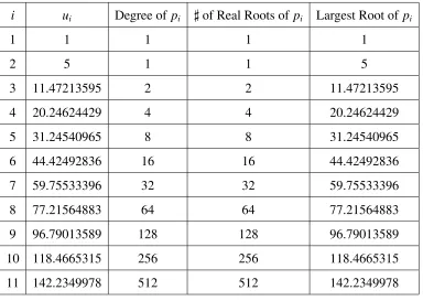
4.1 Roots of minimal polynomials of the sequence of{ui} . . . 49
5.1 Distribution of zeros of p5 . . . 56
5.2 Distribution of zeros of p6 . . . 57
5.3 Distribution of zeros of p7 . . . 58
5.4 Distribution of zeros of p8 . . . 59
List of Tables
1.1 Values ofyn+1for different values of4t . . . 5
4.1 Experimental results for{pi}fori≤11 . . . 48
Chapter 1
Introduction
In this chapter we introduce a sequence of numbers that is given recursively. We briefly
de-scribe the origin of this sequence. In order to do so we need to look at an ordinary differential
equation which is derived from Torricelli’s law for the leaky bucket. Torricelli’s law is a model
in fluid dynamics which gives the relation between the speed of fluid (flowing out) to the height
of the fluid (above the drainage hole) in the bucket.
Assume that we have a cylindrical bucket which contains some fluid. If there is a hole in the
bottom of the bucket, eventually the bucket will run out of water. In [3] the authors commented
on using the following very well-known model:
dy dt =−
√
y (1.1)
where y = Hh, i.e. the ratio of height of fluid to height of bucket. The authors applied the
Euler forward method to solve the model equation. Before talking about the outcome of Euler
forward method, we just recall the method quickly.
Euler forward method is a method for solving ordinary differential equation. For an ordinary
differential equation given by
y0(t)= f(t,y(t))
Figure 1.1: Cylindrical bucket with a drainage hole
and the initial conditiony(t0)=y0, the method gives an approximation of the solution at a given
point. Choosing a value4tfor the size of each step, one can writetn =t0+n4t, then one step of the Euler method fromtntotn+1 is given by
yn+1 =yn+4t f(tn,yn)
whereynapproximates the solution of the equation attn.
Now let us get back to the model (1.1). Using the Euler forward formula and letting the bucket
be full in the beginning (or equivalentlyy0 =1), we get
yn+1 = yn− 4t
√ yn.
For4t = 1, we gety1 =0 which means the bucket empties in just one step. Assuming4t= 12
one can seey1= 12 and calculatingy3gives a negative number which leads to a complex value
fory4. It turns out that for almost all choices of4texcept one family, eventuallyyn < 4t2 for
some integernand thereforeyn+1 <0 which gives a complexyn+2.
Now letting4t= 2
1+√5 implies
y1 =y0− 4t
√
y0= 1− 2
1+ √5
·1=
√
5−1
3
y2 =y1− 4t
√ y1 =
√
5−1
1+ √ 5 − 2 1+ √ 5 s√
5−1
1+
√
5 =0
which means the bucket empties in two steps. Considering4t= 2
1+
√
7+2√5
one can see
y1= y0− 4t
√
y0 =1−
2
1+
q
7+2√5
.1= q
7+2 √5−1
q
7+2 √5+1
and then
y2 =y1−4t
√ y1 =
q
7+2
√
5−1
q
7+2 √5+1
− 2
1+
q
7+2√5
v u u u u u t q
7+2
√
5−1
q
7+2 √5+1
= 4 q
7+2
√
5+1
!−2
finally
y3 =y2− 4t
√ y2 = 4
q
7+2
√
5+1
!−2
− 2
1+
q
7+2
√
5 s
4 q
7+2
√
5+1
!−2
=0
Now we define a sequence{ui}, as
u1 = 1
ui+1= 2+ui+2
√
ui f or i≥2
In [3] the authors showed that in fact the above experimental result holds for anyn.
Theorem 1.0.1 [3] Assume4t= 1+2√
un, then the bucket will be empty in n steps.
Proof We have
yn+1 = yn− 4t
√
yn. (1.2)
Now assumeyn =(4t)2fnand 1 =y0 =(4t)2f0. Hence we get (4t)= √1
f0
.Now we can reformulate equation (1.2) as
(4t)2fn+1 =(4t)2fn−(4t)
p (4t)2f
n
=⇒(4t)2fn+1 =(4t)2fn−(4t)2
p fn
Since (4t),0 then
fn+1 = fn−
p
solving equation 1.3 for fnone gets
fn =
1+ p1+4fn+1 2 2
On the other hand, we haveyn = 0 if and only if fn = 0. The goal here is to find4tsuch that
yn+1= 0 andyn ,0. Hence by putting fn+1 =0 in 1.3 and calculating f0recursively we can get
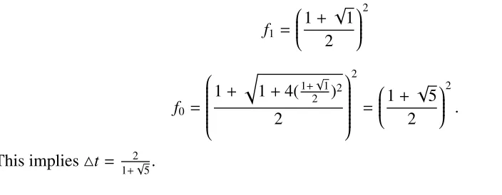
4t. For example if we want the bucket to empty in one step then f2 =0 so
f1= 1+ √ 1 2 2
f0 = 1+ q
1+4(1+ √
1
2 )2
2 2 = 1+ √ 5 2 2 .
This implies4t= 2
1+√5.
Now letukbe the number appearing under the square root in corresponding4t, when bucket is
going to be empty inksteps. In order to be able to find the similar number in the case bucket
gets empty ink+1 steps, we write
f0 = 1+ r
1+41+ √ uk 2 2 2 2 = 1+ q
2+uk +2
√ uk 2 2
This completes the proof.
Table 1.1 shows4t= 1+2√
un for 3≤ n ≤8 which is calculated using the following Maple code
(notice that all computation is performed exactly, floating point is used only for display):
1 Rem_Amount := proc (n) 2 local (i , k , t , x , y);
3 u || 1 := 1; # The symbol || means concatenation .
4 for k from 2 to n do
5 u || k := u || (k -1) +2+2* sqrt (u || (k -1) ); 6 od ;
7 t := 2/(1+ sqrt (u || n));
5
9 for i from 1 to n do
10 x := simplify (y -t* sqrt (y));
11 y := x;
12 od ;
13 print ( evalf (t)); 14 print ( evalf (u || n)); 15 y;
16 end proc :
n un 4t yn+1
3 11.47213595 0.4558867802 0
4 20.24624429 0.3636639572 0
5 31.24540965 0.3035012194 0
6 44.42492836 0.2609193850 0
7 59.75533396 0.2290909432 0
8 77.21564883 0.2043476280 0
Table 1.1: Values ofyn+1for different values of4t
Above results motivated us to investigate more about the sequence of{ui}. As the first step,
we see some experiments that were done (using Maple and Sage). From the recursive formula
of the sequence, one can see the fact that eachun is algebraic over rational numbers (see
def-inition 2.2.3). Our experiments give us the idea to find the sequence of minimal polynomials
of{ui} in a constructive way (see definition 2.2.4). We also noticed that all roots of minimal
polynomials are real.
The mainpurposeof the study is not so much the study of the properties of the{ui}, but rather
developing new tools and applying them: this sequence provides a convenient challenge to
develop recursively-constructed eigenvalue problems. We will learn facts about the sequence,
but more importantly, we will develop a new method for proving that all the roots of a family
of polynomials are real, namely the construction of symmetric B´ezout matrix polynomials and
One purpose of this thesis is to test the utility of the block symmetric linearization of matrix
polynomials expressed in a Lagrange basis [1]. This block symmetrization was only published
in 2009, and is as yet relatively unused; there is no application yet in the literature of which we
are aware.
One simple possibility is that a block symmetric linearization of a symmetric matrix
poly-nomial might allow easy deduction ofdefiniteness,i.e.that all of the non-linear eigenvalues of
the matrix polynomial are positive (or non-negative). Definiteness of a matrix polynomial is
an important property for many purposes: see e.g. [16].
We show in this thesis that, yes, the new block symmetric linearization can be helpful to
de-cide definiteness. Specifically, we look at a new recursively defined family of polynomials that
arises from a non-linear recurrence relation that generates a sequence containing nested square
roots, and show that they are all positive definite by using the aforementioned linearization.
Sequences of nested square roots have been of interest since Vi´ete (also known by the
La-tinized form Vieta) gave the formula (in 1593)
2
π =
√
2
2 ·
q
2+ √2
2 ·
r
2+
q
2+ √2
2 · · · .
Perhaps surprisingly, such sequences are still generating new research results. See for
in-stance [13], [17] and [14].
This thesis proves that a certain sequence of polynomials that define the sequence of nested
square roots described in section 4.1 and section 4.4 is positive definite, thus demonstrating the
utility of the block symmetric linearization.
This thesis is structured as follows: chapter 2 is devoted to the basic notions of field theory
which provides the tools for our calculations. In chapter 3, we provide information about
7
to solving bivariate system of equations. In the last chapter the main results are presented,
namely finding a boundary of{ui}, minimal polynomials of{ui}, roots of minimal polynomials
Preliminaries
In this chapter we provide the preliminary definitions that will be needed in future chapters.
Here we just take a basic knowledge of ring theory and linear algebra for granted and invite the
reader to see [7] and [6] if needed.
The material in this chapter is organized such that the first two sections give general
infor-mation and definitions for Galois theory and the last two sections provide inforinfor-mation for roots
of a family of polynomials and some algorithms to find them.
2.1
Basic Definitions
We recall that a field is commutative ring with identity with the property that every non zero
element has a multiplicative inverse.
Throughout the thesis, we denote the fields of rational numbers, real numbers and complex
numbers (resp.) byQ,RandC.
Theorem 2.1.1 If p is a prime, then the ringZpis a field which is finite.
Example 2.1.1 Assume K is a field and x is an indeterminate. The rational function field of
the polynomial ring K[x], is denoted by K(x)and consists of all f(x)/g(x)such that g(x) , 0
and f(x),g(x)∈K[x].
2.1. BasicDefinitions 9
In general for a given polynomial p(x) ∈ F(x), where F is a field, it is not always the case
that all roots of p(x) lie in F. In order to study the roots of p(x) we need to find a field such
that it contains the roots. To see this better, we note that the roots of x2−2 ∈ Q(x) are±√2
which are not rational numbers. However, there exists a field such that it contains both roots
andQ. The smallest field with this property is denoted byQ(
√
2). One can extend this idea to
the following definition.
Definition 2.1.1 Let F be a field and K be another field such that F ⊆ K. Let A be a subset of K. Then the smallest subfield (with respect to inclusion) of K containing A and F, which is
the intersection of all subfields containing A and F, is denoted by F(A)and is called the field
generated by F and A. If A = {a1,· · · ,an}be a finite set we denote F(A)by F(a1,· · · ,an)and
call it finitely generated. Moreover if A = {a} we write F(a) instead of F(A)and we call it a
simple extension of F.
The above definition does not give F(a) concretely. There is a concrete description of F(A)
in general. We describe the idea for A = {a} and we mention that a similar argument can be
applied to any finiteA⊆K case. We claim that
F(a)={f(a)
g(a) : f(x),g(x)∈F[x],g(a),0}.
We note thatF(a) is indeed the quotient field ofF[a]. So it is enough to show that
F[a]= {f(a) : f(x)∈F[x]}.
In order to do so we defineϕa : F[x] −→ K such thatϕa(f(x)) = f(a). One can verify thatϕ
is indeed a ring homomorphism which is called the evaluation homomorphism ata. It is clear
that Im(ϕa) = {f(a) : f(x) ∈ F[x]} and hence it is a subring of K. Obviously if R ⊆ K be a
subring which containsF anda, then it contains f(a). Therefore we can see that any subring
ofKwhich hasF andainside, should contain{f(a) : f(x)∈F[x]}. So
F[a]= {f(a) : f(x)∈F[x]}.
Theorem 2.1.2 Let F and K be fields, K ⊆ F and{a1,· · · ,an} ⊆ F, then
K[a1,· · · ,an]={f(a1,· · · ,an) : f ∈F[x1,· · · ,xn]}
and
K(a1,· · · ,an)= {
f(a1,· · · ,an)
g(a1,· · · ,an)
: f,g∈F[x1,· · · ,xn],g,0}
2.2
Minimal Polynomials and Algebraic Extensions
We begin this section by providing the definition of field extensions and then we look at a
specific family of field extensions which is called algebraic extensions.
Definition 2.2.1 If K ⊆ F are fields, we say F is a field extension of K. We denote the extension
by F/K and we call K the base field.
It is well known that any fieldF is a vector space over any subfield of itself. So the following
definition will work.
Definition 2.2.2 If F/K is a field extension, then we calldimK(F)(as vector space), the degree
of the extension and we denote it by[F : K]. F is called a finite extension if the degree of F
over K is finite, otherwise it is called an infinite extension.
In this section we are interested in those extensions F/K for which any a ∈ F satisfies a
polynomial inK[x], i.e. there exists a polynomial f(x)∈ K[x] such that f(a) = 0. In order to
understand these extensions better, we need some more formal definitions.
Definition 2.2.3 Assume K/F is a field extension and a ∈ F. We say a is algebraic over K if
there exists a polynomial in K[x]that satisfies at a. If a is not algebraic over K, it is called
transcendental over K. Moreover, if every element of F is algebraic over K, we say F is an
algebraic extension of K and F/K is said to be an algebraic extension.
If a ∈ F is algebraic over K, it satisfies a polynomial over K, but it is not necessarily the
2.2. MinimalPolynomials andAlgebraicExtensions 11
Definition 2.2.4 Assume a is an algebraic element over K. The minimal polynomial of a over K is the monic polynomial with smallest degree in K[x]that satisfies at a.
Example 2.2.1 It is clear that √2satisfies x4−4∈
Q[x], so it is algebraic overQ. However,
x4−4is not the minimal polynomial of √
2since it satisfies x2−2which is of least degree (it
is irreducible over Q). As another example, i = √−1 is algebraic overQ with the minimal
polynomial, x2+1. On the other hand i is algebraic overCwith minimal polynomial, x−i.
Example 2.2.2 It is not trivial that e is transcendental overQ. The first proof was given by
Hermite in 1873. In 1882, Lindemann showed thatπ is transcendental over Q. One can find
proofs for both cases in [12].
Theorem 2.2.1 [12] Let K/F be a field extension andα∈K be algebraic over F. Then
1. The minimal polynomial ofαover F is irreducible over F.
2. If f(x),g(x)∈F[x], such that f(x)be the minimal polynomial ofαover F, then g(α)=0
if and only if f(x)divides g(x).
3. If the degree of minimal polynomial ofαover F is n, then{1, α, α2,· · · , αn−1}is a basis for F(α) over F . Hence[F(α) : F] = deg(p) where p is the minimal polynomial ofα
over F.
Example 2.2.3 Let’s see if 3 √
5is algebraic overQ[x]or not. Assumeα= 3 √
5, now we have
α3 =5
Hence
α3−
5= 0
This means α satisfies p(x) = x3 − 5 ∈
Q. On the other hand, x3 − 5 is irreducible, since
otherwise it must have a root inQ. If a
b ∈Qandgcd(a,b)= 1be a root of p(x), then
(a b)
3−
5=0=⇒ a
3
b3 −5= 0
then
where a|b means a divides b. Let a=5t, then
(5t)3 =5b3 =⇒ 125t3 =5b3 =⇒5|b
which is absurd. Irreducibility of p(x)shows that, it is the minimal polynomial of 3 √
5overQ.
The above argument can be applied in general to any prime q to see xn−q is irreducible over
rationals (alternatively one can apply the Eisenstein criterion [6] to see this). Hence
[Q( n √
q) :Q]=n.
Theorem 2.2.2 Assume F/K is a finite extension. Then F is finitely generated and algebraic
over K.
Proof Let{α1,· · · , αn}be a basis forF overK. Clearly anya∈F can be written as n
X
i=1
ciαi f or some ci ∈K
hence
F =K(α1,· · · , αn).
Ifa∈ F, then{1,a,· · · ,an}is a dependent set overK (recall that dimK(F)= n). This implies,
there existsu1,· · · ,un such that
n
X
i=1
uiai =0
If
f(x)=
n
X
i=1
uixi =0∈K[x]
then f(a)=0. Thereforeais algebraic overK.
The following theorem enables us to state the degree of a field extension in terms of extensions
of middle fields. Moreover, having this machinery, one can prove the converse of the previous
theorem.
Theorem 2.2.3 Assume F⊆ L⊆ K are fields and all extensions are finite. Then
2.2. MinimalPolynomials andAlgebraicExtensions 13
Proof Assume{αi}ni=1and{βj}mj=1are respectively bases forK/LandL/F. We claim that
B={αiβj : 1≤i≤ n, 1≤ j≤m}
is a basis forK/F. As the first step we show BspansK over F. For any elementain K, we
can writeaas a combination ofαi, i.e.
a=
n
X
i=1
aiαi f or some ai ∈L.
On the other hand, any element of L can be written as a linear combination of the βis. In
particular eachaican be written in such a way. Hence
a=
n
X
i=1,j=1
ci jαiβj f or some ci j ∈F.
Now assume
n
X
i=1,j=1
di jαiβj =0
for somedi js inF. The linear independency ofβjs implies that n
X
i=1,j=1
di jαi =0
for any j. Moreover the linear independency ofαis impliesdi j = 0 for alli, j. SoBis a basis
ofKover F, therefore
[K : F]=|B|=n×m= [K :L]×[L: F].
At this point we want to present the converse of theorem 2.2.2. One can find a proof of it which
is based on induction, in [12].
Theorem 2.2.4 Let K/F be a field extension. If eachαibe algebraic over F, then F(α1,· · · , αn)
is a finite field extension of F. Moreover we have
[F(α1,· · · , αn) : F]≤ n
Y
i=1
[F(αi) : F].
One good property of algebraic extensions is the transitivity in the sense of presence of a middle
Theorem 2.2.5 Assume F ⊆ L⊆ K are fields. If K/L is algebraic and L/F is algebraic, then K/F is an algebraic extension.
Proof We have to show any αin K satisfies a polynomial p(x) in F[x]. Sinceαis algebraic overL, f(α)=0 for some
f(x)=
n
X
i=0 aixi
inL[x]. Now consider the fieldL0 = F(a
1,· · · ,an) overFwhich is finite by theorem 2.2.4. We
note that f(x)∈L0[x], soαis algebraic overL0. Thus
[L0(α) :F]= [L0(α) :L0]·[L0 :F]< ∞
On the other hand we haveF(α)⊆ L0(α) which implies finiteness of [F(α) : F] and this means
αis algebraic overF. This argument holds for any element ofK. HenceKis algebraic overF.
Definition 2.2.5 A field F is called algebraically closed if any non-constant polynomial f(x)
in F[x]has a root in F.
Remark 2.2.1 The above definition is saying that a field F is algebraically closed if any
poly-nomial over F factors completely over F. There are equivalent definitions for algebraic closed
fields. One can also say that F is algebraically closed if for any algebraic extension K of F we
have F = K.
Definition 2.2.6 A field extension of F is called an algebraic closure of F if it is an algebraic
extension of F and algebraically closed. We denote the algebraic closure of F byF.¯
Example 2.2.4 It is well-known that C is an algebraic closure of R. However, One should
note thatCis not an algebraic closure ofQ, since it is not algebraic over the field of rational
numbers.
One can use Zorn’s lemma (see [6]) to prove the following important theorem.
Theorem 2.2.6 Every field F has an algebraic closure.
Although the algebraic closure of a field is not unique in general, it is unique up to
2.3. Roots ofPolynomials 15
2.3
Roots of Polynomials
We all learned how to solve a quadratic equation in high school. Although no one taught us
how to do the same thing for cubic or degree four equations at high school, but there we finally
learned that similar methods exist for solving these equations. For a long time, people were
wondering whether is it possible to extend the same idea for higher degree equations or not.
Before getting in to details about roots of polynomials let us provide formal definitions.
Definition 2.3.1 Assume K/F be a field extension and p(x1,· · · ,xn)be a polynomial in F[x1,· · · ,xn].
α1,· · · , αn ∈K is called a root of p if p(α1,· · · , αn)= 0.
By solving a polynomial, we mean finding the set of roots of it. A univariate polynomial is
called solvable by radicals if it can be solved by a combination of the following operations:
• Operations of the field.
• Using n-th roots in the field for some positive integer (e.g. square root, third root and
etc.)
Ruffini was the first one who argued the fact that a general univariate polynomial of degree five
or higher is not solvable by radicals. Although his proof was not complete, one should admit
it was a great achievement at that time. Later in 1824, Abel gave a complete proof. However
the most prominent and inspiring proof was given by Galois. He not only proved the above
statement, but also he could solve some other geometric problems which were unsolved for
centuries. The results of his work these days is called Galois theory.
Knowing that degree five (and higher) univariate polynomials are (in general) unsolvable with
radicals, people were looking for other methods to solve the problem. Indeed there are diff
er-ent approaches for any problem. In this special case one can use numerical methods to find
approximations of roots or use symbolic computations to find roots. It is worth mentioning that
there are methods combining these two approaches which are called hybrid methods.
[8]) as a method of solving polynomial equations, by reducing them to univariate polynomials
or to linear system. As a matter of fact, in many applications, in practice we just need an
ap-proximation of a root. However, there are some applications which need exact solutions.
All we have discussed until now is about solving one single equation. What if we have a
system of non-linear equations and we are interested in the set of solutions?
Though modern algebraic geometry uses the language of schemes ([10]), the classic
alge-braic geometry define varieties as the set of solution of a family of polynomials. Algealge-braic
geometers are interested in studying varieties and their properties. In some cases people want
to calculate the set of points of a variety which is equivalent of solving a system of non-linear
equations. There are relations between the number of variables in the non-linear systems and
the dimension of the corresponding geometric object. Thus, in dimensions higher than one we
want to be able to solve a system of multivariate polynomials over a field.
Again Gr¨obner basis is a powerful tool in solving a non-linear system of multivariate
poly-nomials. In the next section we will describe the related application of resultant in solving a
bivariate system of polynomials.
2.4
Solving Bivariate Polynomials
In this section we want to see a method which can be applied to solve a system of bivariate
equations. We do not claim that this is the most efficient one. In fact this method will be used
in the last chapter in order to calculate the desired minimal polynomials.
Definition 2.4.1 Assume two non-zero polynomials f(x)and g(x) are given in R[x], where R
is a UFD1. If
f(x)=
n
X
i=0
aixi and g(x)= m
X
i=0 bixi
then the Sylvester matrix of f and g which we denote bySylx(f,g)is the m+n by m+n matrix
an an−1 · · · a1 a0 an an−1 · · · a1 a0
· · · ·
an · · · a0 bm bm−1 · · · b1 b0
bm bm−1 · · · b1 b0
· · · ·
bm · · · b0
Definition 2.4.2 For f(x),g(x)∈R[x], where R is a UFD, the resultant of f and g with respect
to x which is denoted byresx(f,g), is the determinant of the Sylvester matrix.resx(0, f)=0for
non-zero f ∈R[x]and by definition,resx(f,g)= 1for non-zero constants in R.
Example 2.4.1 Using Maple built in functions, SylvesterMatrix and resultant, we calculate
them for two polynomials. We can find the resultant directly or by forming the Sylvester
matrix and computing its determinant.
> with(LinearAlgebra):
> f:=xˆ4-6*xˆ2+1;
f := x4−6x2+1
> g:=xˆ5+2*xˆ3-x;
g := x5+2x3− x
A :=
1 0 −6 0 1 0 0 0 0
0 1 0 −6 0 1 0 0 0
0 0 1 0 −6 0 1 0 0
0 0 0 1 0 −6 0 1 0
0 0 0 0 1 0 −6 0 1
1 0 2 0 −1 0 0 0 0
0 1 0 2 0 −1 0 0 0
0 0 1 0 2 0 −1 0 0
0 0 0 1 0 2 0 −1 0
> Determinant(A); 784 > resultant(f,g,x); 784
One can see that the determinant of Sylvester matrix of two polynomials is equal to resultant
of them.
The resultant is also helpful in computing the greatest common divisors of two polynomials,
but here we are interested in its applications to solving system of equations.
We just recall that a solution of a system ofnpolynomials inmvariables
f1(x1,· · · ,xm)=0
f2(x1,· · · ,xm)=0
...
2.4. SolvingBivariatePolynomials 19
over a field F is an m-tuple (α1,· · · , αm) in some field extension F such that it satisfies all
equations, i.e. for eachiwe have fi(α1,· · · , αm)=0.
Theorem 2.4.1 (Sylvester’s Criterion) [8] Let f(x),g(x)∈R[x]where R is a UFD. Then f(x)
and g(x)have a non-trivial common factor if and only ifresx(f,g)= 0.
Example 2.4.2 In this example we can see that for two polynomials f and g which have a
common factor x−1, the resultant of these two is zero.
> f := xˆ5-3*xˆ4+2*xˆ3+x-1;
f := x5−3x4+2x3+ x−1
> g := xˆ6+xˆ5-2*xˆ4-xˆ2+x;
g := x6+ x5−2x4− x2+ x
> resultant(f,g,x);
0
One can have the following general fact about resultants for multivariate polynomial systems.
Theorem 2.4.2 (Fundamental Theorem of Resultants) [8] Let F be an algebraically closed¯
field, and let
f(x1,· · · ,xn)= n
X
i=0
ai(x2,· · · ,xn)x1i,
g(x1,· · · ,xn)= m
X
i=0
bi(x2,· · · ,xn)x i
1
be elements ofF¯[x1,· · · ,xn]of positive degrees in x1. Then if(α1,· · · , αn)is a common zero of
f and g, their resultant with respect to x1 satisfies
resx1(f,g)(α2,· · · , αn)=0
Conversely if the above resultant vanishes at (α1,· · · , αn), then at least one of the following
holds:
3. an(α2,· · · , αn)=bm(α2,· · · , αn)= 0;
4. There existsα1 ∈F such that¯ (α1,· · · , αn)is a common zero of f and g.
The above result gives us a way to reduce some system of bivariate polynomials into solving
a univariate polynomial. In fact let f(x,y) andg(x,y) be two bivariate polynomials. Assume
there exists a solution for their system which we call (α1, α2). By the above theorem we have
resx(f,g)(α2) = 0. Thus in order to find (α1, α2) we can calculate resx(f,g) and find its roots.
For each root of the resultant, we can plug it in to the system and see if they have a common
root. Obviously this works if we have an efficient way to solve a univariate equation. The
following example illustrates this idea.
Example 2.4.3 Assume that polynomials f(x) = x2− y2−1 and g(x) = x2 +yx−7are
given. We want to find all (α, β)such that it satisfies both f and g. In order to do so, we
first compute the resultantresx(f,g).
> with(LinearAlgebra):
> f := proc (x, y) options operator, arrow; xˆ2-yˆ2-1 end proc;
f := (x,y)7→ x2−y2−1
> g := proc (x, y) options operator, arrow; xˆ2+y*x-7 end proc;
g := (x,y)7→ x2+yx−7
> R := resultant(f(x, y), g(x, y), x);
R := −13y2+36
Having the resultant, we can find its roots which gives us all candidates forβ.
> ysolve := [solve(R)];
ysolve := [−6 √
13
13 ,
6
√
13
13 ]
It is time to check if we can find anαwhich completesβas a solution. By plugging in
the values of resultant in f , we find candidates forα.
2.4. SolvingBivariatePolynomials 21
x2− 49
13
> xsolve := [solve(f(x, ysolve[1]))];
xsolve := [7
√
13
13 ,−
7 √13
13 ]
The final step is to check the pairs formed from candidates for αandβ, to find which
pair satisfies both equations.
> f(xsolve[2], ysolve[1]);
0
> g(xsolve[2], ysolve[1]);
0
> f(xsolve[1], ysolve[2]);
0
> g(xsolve[1], ysolve[2]);
0
This approach is combinatorially expensive in the number of variables. We will see a better
Matrix Polynomials
3.1
Basic Definition
3.1.1
Matrix Polynomial
Matrices are very useful in mathematics and its applications [9]. There are various types of
matrices. Among those, there are a family of matrices which instead of having numbers as
their entries, they have polynomials as entries. One of the applications of this family is finding
common roots of polynomials. We want to apply this method, so we will convert rootfinding
of a system of polynomial equations in two variables into a so-called nonlinear eigenvalue
problem and solve that by linearization. All of these concepts will be defined in this chapter.
Definition 3.1.1 A univariate matrix polynomialM(x)of degree n is defined as
M(x)=
n
X
i=0
Mixi (3.1)
whereMiare numerical matrices, i≥0.
It is easy to see that any matrix polynomial is a matrix with univariate polynomials as entries.
This duality is simple, but is not useless.
Example 3.1.1 In this example we provide a matrix polynomial which is represented by a
matrix with polynomial entries. We use Maple to rewrite it as a polynomial with matrix
coefficients.
3.1. BasicDefinition 23
> with(LinearAlgebra):
> with(MatrixPolynomialAlgebra):
> M:=<<xˆ2-2*x|x-1>,<x+3|xˆ3-1>>;
M :=
x2−2x x−1
x+3 x3−1
> add(xˆi*A[i], i = 0..3);
x3A3+x2A2+xA1+A0
where
> A[3]:= coeff(M,x,3);
A[3] := 0 0 0 1
> A[2]:= coeff(M,x,2);
A[2] := 1 0 0 0
> A[1]:= coeff(M,x,1);
A[1] :=
−2 1
1 0
> A[0]:= coeff(M,x,0);
A[0] :=
0 −1
3 −1
3.1.2
Generalized Eigenvalues and Eigenvalue Problem
We recall that the eigenvalue problem for a matrix A is finding scalars λ and corresponding
vectorsvsuch that they satisfy the following (if they exist):
Av= λv.
One can easily convert above expression to
(λI−A)v=0.
In general one can form the determinant of (xI−A), which is a univariate polynomial inx, and
the roots of this polynomials are the eigenvalues. In practice finding the eigenvalues by above
method needs polynomial factorization which is problematic. There are numerical methods
that one can apply to get the eigenvalues. The most famous one among these methods is the
QR algorithm; see [4].
If we replace the identity matrix above with another matrix B, we may still be interested in
findingλandvsuch that
Av= λBv.
Such a λ is called a generalized eigenvalue. There is another version of this notion, where
a pair (α, β) (that are not both zero) of field elements, is called a generalized eigenvalue of a
matrix pair (A,B) if there exists a non-zero vectorvsuch that
αAv=βBv.
We may take|α|2+|β|2 =1 and Re(α)≥0, without loss of generality. Ifβ
,0,λ= αβ. Ifβ= 0,
we say (A,B) has an infinite eigenvalue.
There is a similar (to QR) algorithm for solving the generalized eigenvalue problem
numer-ically, which is called the QZ algorithm; see [4].
Definition 3.1.2 A pair of matrices(A,B)whereA,B ∈Cn×n
, is called a matrix pencil if they
define a generalized eigenvalue problem
3.1. BasicDefinition 25
andλis called a generalized eigenvalue for the pencil(A,B)or equivalently(α, β)with|α|2+
|β|2 =1andRe(α)≥0.
It is not hard to see t is a generalized eigenvalue of the pencil(A,B)if and only if t is a root
ofdet(yB−A). So one can restate the generalized eigenvalue problem as finding roots of the
determinant of(yB−A).
The following definition presents formally the above notions and introduces some notations.
Definition 3.1.3 AssumeAandBare two matrices. Then the set of eigenvalues ofAwhich is
denoted byΛ(A), is the set
Λ(A)= {z: det(zI−A)= 0}
The set of generalized eigenvalues of the pair(A,B), is denoted byΛ(A,B)is
Λ(A,B)={z: det(zB−A)= 0}
and finally the set of nonlinear eigenvalues of a matrix polynomialP(z)=zdAd+· · ·+zA1+A0 is denoted byΛ(P)and is given by
Λ(P) :={z: det(P(z))=0}.
A matrix polynomial,M, is called regular if det(M) is not identically zero and is called singular
otherwise. One should note that there exist pencils which are singular. As an example for
A=
0 0
0 1
andB=
0 0
0 1
then
det(zA−B)= det
0 0
0 z−1
=0.
3.1.3
The Companion Pencil
One of the simplest and most useful matrix polynomials is the companion pencil, which we
introduce in this section. For simplicity we first define the companion pencil for an ordinary
Definition 3.1.4 Let p(x)be a univariate polynomial over complex numbers. Writing p(x)as
p(x)=
n
X
i=0 aixi
we define the pencil(C0,C1)∈(Cn×n)2as
C0 = 0 1 0 1 ... ... ... 1
−a0 −a1 · · · −an−1
C1 = 1 1 ... 1 an
Note that if an = 1(the polynomial is monic) then this is also called the Frobenius companion
pencil. There are others (Fiedler, [5]).
If(C0,C1)is the companion pencil of p(x), a simple calculation shows that
p(x)= det(C1x−C0).
We have similar definition for a matrix polynomialP(x).
Definition 3.1.5 LetP(x)be a matrix polynomial. That is, suppose
P(x)=
n
X
i=0
Aixi
where for each i,Ai ∈Cn×n.Then we define the companion pencil (also known as a
3.2. B´ezoutMatrix 27
C0= 0 I 0 I ... ... ... I
−A0 −A1 · · · −An−1
C1= I I ... I An
One can see that
det(P(x))=det(xC1−C0)
We will see this equality in section 3.4. Note that there are other linearizations.
3.2
B´ezout Matrix
In this section we want to introduce the B´ezout matrix for two polynomials. Let f(x) andg(x)
be two polynomials of degreemandnrespectively:
f(x)=
m
X
i=0 aixi
g(x)=
n
X
i=0 cixi
The Cayley quotient of f andgis defined as follows, whered =max(m,n):
C(x,y)= f(x)g(y)−g(x)f(y) x−y
Sincex= yobviously makes
thenx−yis a factor of the numerator.
Hence, we can write the Cayley quotient as:
d
X
i=1
d
X
j=1
bi jxi−1yj−1
The B´ezout matrix is the followingd×dmatrix:
B= (bi j)d×d
Then
C(x,y)=
1 x x2 · · · xd−1
B
1
y
y2
...
yd−1
Example 3.2.1 Let’s construct the B´ezout matrix in different ways. For a given pair of polynomials we form the Cayley quotient and then construct the B´ezout matrix from it. On
the other hand we can use the built in function for the B´ezout matrix in Maple with different
options.
> with(LinearAlgebra):
> f := randpoly(x, degree = 2);
f := −7x2+22x−55
> g := randpoly(x, degree = 3);
g := −94x3+87x2−56x
> C := simplify(expand(f*subs(x = y, g)-subs(x = y, f)*g)/(x-y));
658x2y2−2068x2y−2068xy2+5170x2+6692xy+5170y2−4785x−4785y+3080
> d := max(degree(f, x), degree(g, x));
3.3. B´ezoutMatrix inLagrangeBasis 29
> Bez := Matrix(d, d, (i, j) -> coeff(coeff(C, x,d-i), y, d-j));
B2 :=
−658 2068 −5170
2068 −6692 4785
−5170 4785 −3080 > B1:=BezoutMatrix(f,g);
B1 :=
4778 −3553 0
−1459 4778 0
−7 22 −55
> B2:=BezoutMatrix(f,g, method = symmetric);
B2 :=
−658 2068 −5170
2068 −6692 4785
−5170 4785 −3080
Remark Obviously the above example shows different matrices for the corresponding B´ezout
matrix to a fixed pair of polynomials. However, one can easily verify that the determinants of
the matrices are equal up to a constant.
We note that we are looking at Cayley quotient in monomial basis. We are able to write the
Cayley quotient in the Lagrange basis and construct a similar B´ezout matrix. This will be
investigated in the next section (see [15]).
3.3
B´ezout Matrix in Lagrange Basis
As we mentioned in the previous section, it is possible to write the Cayley quotient in a
La-grange basis. This has some computational benefits. In [15] Shakoori described the B´ezout
matrix in Lagrange basis. What we are presenting here is a brief discussion of her paper and
we encourage the reader to see [15] for more details.
We defined the B´ezout matrix using the Cayley quotient.
Recall thatd = max(deg(f),deg(g)). It is not hard to see thatC(x,y) is a polynomial in terms
ofxand also inyof degree at mostd−1. Indeed one can write the Cayley quotient as:
C(x,y)=
1 x x2 · · · xd−1 B 1 y y2 ...
yd−1
whereBis the corresponding B´ezout matrix for f andg.
A closer look gives the idea of interpolating the polynomials xi andyi for 0 ≤ i ≤ d−1. In
order to do so we set two sets of nodes, namelyX = {x1,· · · ,xd}andY ={y1,· · · ,yd}. We also
writeLi(x) (Li(y) resp.) i.e.
Li(x)=
Y
0≤j≤d i,j
x−xj
xi−xj
for the i-th Lagrange polynomial for xi (yi resp). So after all, we can have interpolation for
eachxi andyi. One can write the interpolations as follow:
1 x x2 ...
xd−1 =
1 1 · · · 1
x1 x2 · · · xd
x21 x22 · · · x2d
... ... · · · ... xd−1
1 x
d−1
2 · · · x
d−1 d
L1(x)
L2(x)
L3(x)
...
Ld(x)
In the above expression the middle matrix is the transpose of well-known Vandermonde matrix.
One can write a similar expression for row matrix of xis:
1 x x2 · · · xd−1
= L1(x) L2(x) L3(x) · · · Ld(x)
1 x1 · · · xd1−1 1 x2 · · · xd2−1 1 x3 · · · xd3−1
... ... · · · ...
1 xd · · · xdd−1
Now we can get back to write the Cayley quotient in the Lagrange basis, by replacing the
appropriate matrices we wrote above. Hence
C(x,y)=
L1(x) L2(x) L3(x) · · · Ld(x)
VXBVTY
L1(y)
L2(y)
L3(y)
...
Ld(x)
where
VX =
1 x1 · · · xd1−1 1 x2 · · · xd2−1 1 x3 · · · xd3−1
... ... · · · ...
1 xd · · · xdd−1
We call BL = VXBVTY the B´ezout matrix in Lagrange basis. We do not compute it this way,
however, except as demonstration.
Example 3.3.1 The following Maple code outputs the B´ezout matrix for a pair of polynomials
(p, f)where p is a univariate polynomial in x, and f is a polynomial derived from the relation
between ui and ui+1such that f(ui,ui+1)=0. In chapter4we will talk about f in more detail.
1 with ( LinearAlgebra ):
2 ## This function returns Bezout matrix based on monomial basis , for the
input p which is a polynomial and f ( which is fixed ).
3 bez := proc (p)
4 local f , B , n , c , i , j;
5 f := (y -2) ˆ2 -2* x*y+x ˆ2;
6 n := max ( degree (f) , degree (p));
7 B := Matrix (n); ## It is a blank square matrix of size n.
8 c := simplify ( expand (( f *( eval (p , x = s)) -p *( eval (f , x = s))) /(x -s)));
9 ## This loop assigns coefficients of Cayley quotient to B.
10 for i from 0 to n -1 do
11 for j from 0 to n -1 do
13 od ; 14 od ; 15 B;
16 end proc :
1 BezL := proc (p , r)
2 local v , vT , BM , BL , m , n;
3 BM := bez (p);
4 m := degree (p);
5 if nops (r) = m then
6 v := VandermondeMatrix (<r >) ;
7 vT := Transpose (v);
8 BL := Multiply (v , Multiply (BM , vT ));
9 else
10 return (0) ;
11 end if ;
12 end proc :
> BezL(390*xˆ2-1508*x+1409, [2, 4]);
−52y2+510y−604 −832y2+6750y−6938
−832y2+6750y−6938 −1612y2+16110y−19304
In [15] using above discussion, Shakoori proved the following efficient way of computing the
B´ezout matrix in Lagrange basis.
Theorem 3.3.1 [15] For two bivariate polynomials f and g by their values at some known
points, the B´ezout matrix in Lagrange basis is defined by
BLi j = f(xi)g(yj)− f(yj)g(xi)
xi−yj
i f i, j and 0≤ i, j≤d
BLii = fi0gi− fig
0
i 0≤ i≤d.
where fi = f(xi), gi = g(xi), fi0 = f0(xi)and g0i = g0(xi). Moreover, the null vectors ofBLmay
be parametrized by the Lagrange basis polynomials evaluated at the common roots of f and g.
Shakoori also introduced an effective method for calculating the values of the derivatives of f
3.4. Linearization of aMatrix polynomial 33
Assume we have a polynomial p(x) of degree n and set of distinct nodes{x0,· · · ,xn}. If we
denote the values of pon xi by pi and the values of p0 by p0i, then we can compute the values
of the derivative using the following formula:
D p0 p1 ... pn = p0 0
p01
...
p0n
where
Dii=
X
i,j
1 xi−xj
Di j =
Y
k,j k,i
(xi− xk)/
Y
k,j
(xj−xk)
3.4
Linearization of a Matrix polynomial
We already introduced matrix polynomials and their generalized eigenvalues. We are
inter-ested in studying the set of non-linear eigenvalues which is called the spectrum of the matrix
polynomial. Normally we have no control on the degree of the given matrix polynomial. It
would be helpful if we could use a linear matrix polynomial, i.e. a matrix polynomial of the
formAx−B(whereAandBare numerical matrices) such that the spectra ofAx−Band the
original matrix polynomial are the same.
Definition 3.4.1 [9] Let
P(x)=
n
X
i=0
Aixi
be a regular (i.e. its determinant in not identically zero) m×m matrix polynomial. An mn×mn
linear matrix polynomialS1x+S0is called a linearization ofP(x)if
P(x) 0
0 Im(n−1)
=E(x)(S1x+S0)F(x)
AssumeP(x) is a given matrix polynomial of degreen. So we can writeP(x) as:
P(x)=Anxn+· · ·+A1x+A0.
In the simplest case ifAnis a non-singular matrix, we can form the companion matrix for
A−1n Anxn+· · ·+A−1n A1x+A−1n A0 i.e.
Cp =
0 I 0 · · · 0
0 0 I · · · 0
... ... ... ... ...
0 0 · · · 0 I
−A−1n A0 −A−1n A1 −A−1n A2 · · · −A−1n An−1
HavingCpwe can verify thatxI−Cpis a linearization forP(x), using
F(x)=
I 0 0 · · · 0
−xI I 0 · · · 0
... ... ... ... ...
0 0 · · · I 0
0 0 · · · −xI I
and
E(x)=
Bn−1(x) Bn−2(x) · · · B0(x)
−I 0 · · · 0
0 −I · · · ...
... ... ... ...
0 0 · · · −I 0
whereB0(x)=IandBt+1(x)= xBt(x)+An−t−1for 0 ≤t≤ n−2 and forming
P(x) 0
0 Im(n−1)
F(x)=
An 0
0 Im(n−1)
E(x)(Ix−Cp).
Obviously the linearization of a matrix is not unique. More precisely having a linearization
any non-singular C andD, C(Ax−B)D is a linearization again. In particular, if we use the following transformations: C=
I 0 · · · 0 0
0 I · · · 0 0
... ... ... ... ...
0 0 · · · I 0 0 0 · · · 0 An
AndD= I(of appropriate size) then
C(Ix−Cp)D= x
I 0 · · · 0 0
0 I · · · 0 0
... ... ... ... ...
0 0 · · · I 0 0 0 · · · 0 An
−
0 I 0 · · · 0
0 0 I · · · 0
... ... ... ... ...
0 0 · · · 0 I
−A0 −A1 · · · −An−2 −An−1
The above matrix polynomial is the companion pencil ofP(x) which we already introduced in
section 3.1.3
Example 3.4.1 For the given matrix polynomial we calculateCpand then compare the
de-terminants of p and xI−Cp. We also do the same thing forC1x−C0.
> with(LinearAlgebra):
> A2 := RandomMatrix(3, 3, generator = 1 .. 10);
A2 :=
10 9 10
1 7 6
6 1 6
> Determinant(A2); 220
A1 :=
3 3 8
6 10 7
> A0 := RandomMatrix(3, 3, generator = 1 .. 2);
A0 :=
1 1 1
2 1 1
2 2 1
> P := A2*xˆ2+A1*x+A0;
P :=
10x2+7x+1 9x2+x+1 10x2+7x+1
x2+3x+2 7x2+3x+1 6x2+8x+1
6x2+6x+2 x2+10x+2 6x2+7x+1
> Cp :=<<ZeroMatrix(3)|IdentityMatrix(3)>
> ,<Multiply(-A2ˆ(-1), A0)| Multiply(-A2ˆ(-1), A1)>>>;
Cp :=
0 0 0 1 0 0
0 0 0 0 1 0
0 0 0 0 0 1
21
55 2/11
6 55 − 6 55 64 55 53 55 7 22 7
22 1/11
9 22 47 22 7 11 −169 220 − 25 44 − 16 55 − 211 220 − 701 220 − 123 55 > Determinant(P);
220x6+46x5−594x4−373x3−30x2+10x+1
> D := Determinant(x*IdentityMatrix(6)-Cp);
D := x6+ 23x 5
110 −
27x4
10 −
373x3
220 −
3x2
22 + x/22+
3.4. Linearization of aMatrix polynomial 37
> 220*D;
220x6+46x5−594x4−373x3−30x2+10x+1
> C0 :=<<ZeroMatrix(3)|IdentityMatrix(3)>,<-A0|-A1>>>;
C0 :=
0 0 0 1 0 0
0 0 0 0 1 0
0 0 0 0 0 1
−1 −1 −1 −7 −1 −7
−2 −1 −1 −3 −3 −8
−2 −2 −1 −6 −10 −7
> C1 := DiagonalMatrix([IdentityMatrix(3), A2]);
C1 :=
1 0 0 0 0 0
0 1 0 0 0 0
0 0 1 0 0 0
0 0 0 10 9 10
0 0 0 1 7 6
0 0 0 6 1 6
> Determinant(C1*x-C0);
220x6+46x5−594x4−373x3−30x2+10x+1
As we can see in the previous example, the linearization and the original matrix have the same
determinant and this is not a coincidence. It is always the case.
3.5
Linearization with Lagrange Basis
So far we defined linearizations in the monomial basis. In this section we want to talk about a
linearization in a Lagrange basis.
SupposeP(x) to be a matrix polynomial of degreenwhich is given in monomial basis.
P(x)= Anxn+· · ·+A1x+A0
Let’s haven+1 sample nodes for writingP(x) in Lagrange basis. Assuming x0,· · · ,xn to be
distinct points, the values ofP(x) over these points will be shown byPi, i.e. Pi = P(xi). Now
Lagrange polynomials are presented as
Li(x)= n
Y
j=0,j,i
x−xj
xi−xj
It is convenient to define
ωi = n
Y
j=0,j,i
1 xi−xj
.
ThenP(x) in Lagrange polynomial will be
P(x)=
n
X
i=0
Li(x)Pi
Amiraslani in his Ph.D. dissertation [2], calculated the companion pencil forP(x) in Lagrange
basis:
xC1−C0=
(x−x0)I 0 · · · 0 −P0
0 (x−x1)I · · · 0 −P1
... ... ... ... ...
0 0 · · · (x−xn)I −Pn
ω0I ω1I · · · ωnI 0
3.5. Linearization withLagrangeBasis 39
which is a linearization forP(x) (see [1]).
Amiraslani et al. in [1] introduced a matrixAas
A= ω−1
0 P0 0 · · · 0 0 0 ω−11 P1 · · · 0 0
... ... ... ... ...
0 0 · · · ω−1n Pn 0
0 0 · · · 0 −I
such that
(xC1−C0)A=
x−x0
ω0 P0 0 · · · 0 P0
0 x−x1
ω1 P1 · · · 0 P1
... ... ... ... ...
0 0 · · · x−xn
ωn Pn Pn
P0 P1 · · · Pn 0
A Sequence of Symmetric B´ezout Matrix
Polynomials
4.1
Introduction
In this chapter we state the main results. The first observation for the sequence ofuis is that all
of the terms are algebraic overQ. This fact is stated formally in section 4.2. In section 4.3 a
lower and upper bound foruis is presented. Section 4.4 is devoted to a constructive approach
for finding the sequence of minimal polynomials. Having minimal polynomials, showing that
“the roots of minimal polynomials are all real” is the subject of section 4.5 and finally section
4.6 is devoted to finding symmetric linearization of the B´ezout matrix.
Before getting in to details let us recall the definition of the sequence ofuis.
u1 = 1
un+1 =2+un+2
√
un (4.1)
It is easy to see that the first few terms in the sequence are:
u1 = 1
u2 = 5
4.2. {ui}isAlgebraic over the set ofRationalNumbers 41
u3 =7+2
√
5
u4 =9+2
√
5+2
q
7+2
√
5 (4.2)
By looking at these numbers, one might guess the degree of minimal polynomial of eachuiover
Q. We will find the degrees by considering a tower of field extensions over rational numbers,
in section 4.3.
4.2
{
u
i}
is Algebraic over the set of Rational Numbers
In this section we want to show that alluis are algebraic overQ. For this reason we can look at
field extensions generated byuioverQfor alli≥ 2.
Theorem 4.2.1 For each i, ui is algebraic overQ.
Proof The proof is by induction oni. We first show thatu3is algebraic over rational numbers.
We can do as below:
u3 =7+2
√
5=⇒u3−7=2
√
5=⇒ (u3−7)2= 20
Hence
u23−14u3+29= 0
Sou3 satisfies
x2−14x+29=0.
Q Q(ui)
Q(ui)(ui+1)=Q(ui,ui+1)
By our assumption, we know thatQ(ui)/Qis an algebraic extension.
On the other hand, we have
ui+1 =2+ui+2
√ ui
=⇒ (ui+1−2−ui)2 =4ui
=⇒((ui+1−2)−ui)2= 4ui
=⇒ (ui+1−2)2−2(ui+1−2)ui+u2i −4ui =0
=⇒ (ui+1−2)2−2ui+1ui+u2i =0
So ui+1 satisfies (x− 2)2 −2xui + u2i = 0. Thus ui+1 is algebraic over Q(ui). By induction
assumptionQ(ui)/Qis algebraic. Now Theorem 2.2.5 tells usui+1is algebraic overQ.
\
4.3
Boundary of
{
u
i}
In this section we want to find the upper and lower bound forun.
Theorem 4.3.1 If n≥5, then
un≥ (n+1)2−5.
Proof We can prove this statement by using induction onn.
Letn= 5. One can see that