Scholarship@Western
Scholarship@Western
Electronic Thesis and Dissertation Repository
11-29-2016 12:00 AM
Volatility Modelling with Applications to Equity and Foreign
Volatility Modelling with Applications to Equity and Foreign
Exchange Markets
Exchange Markets
Sergii Pypko
The University of Western Ontario
Supervisor Dr. Lars Stentoft
The University of Western Ontario Joint Supervisor Dr. Timothy Conley
The University of Western Ontario Graduate Program in Economics
A thesis submitted in partial fulfillment of the requirements for the degree in Doctor of Philosophy
© Sergii Pypko 2016
Follow this and additional works at: https://ir.lib.uwo.ca/etd
Part of the Econometrics Commons, and the Finance Commons
Recommended Citation Recommended Citation
Pypko, Sergii, "Volatility Modelling with Applications to Equity and Foreign Exchange Markets" (2016). Electronic Thesis and Dissertation Repository. 4314.
https://ir.lib.uwo.ca/etd/4314
This Dissertation/Thesis is brought to you for free and open access by Scholarship@Western. It has been accepted for inclusion in Electronic Thesis and Dissertation Repository by an authorized administrator of
My thesis consists of three chapters describing volatility forecasting during periods of
fi-nancial booms and busts, the economic and statistical benefits of flexible data generating
process of index returns, and multivariate model of exchange rate returns and their options.
In the first chapter, I propose a non-linear threshold model for realized volatility of
S&P 500 index, allowing us to obtain a more accurate volatility forecast, especially during
periods of financial crisis. The changes in volatility regimes are driven by negative past
returns, where the threshold equals approximately −1%. This finding remains robust to different functional forms of volatility and different set of indices from both developing
and developed countries. The additional flexibility of the model allows me to produce a
more accurate one and multiple-days-ahead forecasts compared to the linear specification
and GARCH family models. Finally, I derive an approximated closed form solution for
multiple-step-ahead forecast, which is based on the normal-inverse Gaussian conditional
distribution of returns.
In the second chapter, I develop a novel discrete-time model for the asset return based
on the high-frequency data and mixture of normal (MN) distributions of the latent volatility.
This model accurately replicates distributions of both returns and realized volatility under
the objective measure. To compute option prices, I specify a Radon-Nikodym derivative,
which includes both Gaussian and non-normal innovations, correspondingly. Crucially,
my approach avoids calibration of all model’s parameters. I price European Put options
using Monte Carlo simulations and assess pricing performance of MN and nested
Gaus-sian models during turbulent financial markets in 2008-2011 years. MN model does not
only substantially reduce option pricing errors compared with Gaussian model, but
pro-vides an appealing econometric framework to assess evolution of investors’ risk. Next, I
tent of option prices and MN model. Finally, I build a simple quantitative strategy, which
substantially outperforms returns of S&P 500 index (76% compared with 2%) during
tur-bulent 2008-2011 years, while remaining market-neutral and had the same volatility as a
benchmark returns.
In the third chapter, which is a joint work with Chang, Feunou and Fontaine, we
pro-pose a new multivariate factor model of exchange rate returns and their option-implied
variances. This model documents a tight factor structure in the variance of exchange rate
returns and then relate it to the economic factors. In particular, we show that the common
factors driving variances of exchange rate returns include the variances of global factors
and the common factors driving variances of country-specific shocks. We build a tractable
multivariate asset pricing model based on these stylized facts for the underlying exchange
rate returns. Our multivariate model provides a reasonable fit compared with performance
of univariate models estimated for each series separately. Crucially, our model has a
num-ber of appealing benefits which are not attainable in the univariate framework. For example,
this model can be used to devise a better portfolio construction or hedging strategy for a
portfolio containing both currencies and currency options.
keywords: volatility modelling, derivatives pricing, risk management, forecasting
This thesis contains Chapter 3 co-authored with Bo Young Chang, Bruno Feunou and
Jean-S´ebastien Fontaine.
I am very grateful to John Knight for his support, guidance and motivation. He was a
person who inspired me to start my research.
I am grateful to my supervisors Lars Stentoft and Timothy Conley for their valuable
comments and support during my studies. I want to thank Lars Stentoft for the
oppor-tunity to be engaged in the research area of derivatives pricing as his research assistant,
which became the fundamental part of my dissertation. I also grateful to his comments
and discussions, which were important factors for me to develop both as economist and
econometrician.
I like to thank to my committee member Salvador Navarro for his support and
sug-gestions. I am also thankful to my co-authors from the Bank of Canada, Bo Young Chang,
Jean-S´ebastien and Bruno Feunou, for the opportunity to work with them on my third
chap-ter during my time at the Bank of Canada. I am grateful to Galyna Grynkiv and Miguel
Cardosso for their comments and recommendations during writing of this dissertation. I
would also to thank participants, referees and discussants for their insightful comments and
recommendations at the number of conferences and workshops, including Midwest Finance
Association 2015 Annual Meeting, 3rdAnnual Doctoral Workshop in Applied
Economet-rics, Western University 2nd Financial Econometrics and Risk Management conference,
Western University, Bank of Canada and 50thCanadian Economic Association.
Finally, I would like to thank my wife, Galyna and my son, Roman for their
uncon-ditional support, tremendous help and huge inspiration to me during the writing of this
dissertation. I also want to thank my mother-in-law, Olga and father-in-law, Petro for
tak-ing care of my son, while I was worktak-ing on my thesis. I also want to thank my parents,
Anatolii and Alevtyna and my sister, Olena for their support. I dedicate this work to them.
Certificate of Examination ii
Abstract iii
Acknowledgement vi
List of Tables xii
List of Figures xiv
List of Appendices xvi
1 Volatility Forecast in Crises and Expansions 1
1.1 Introduction . . . 1
1.2 Model . . . 4
1.2.1 HAR-RV Model with Regime Switching . . . 5
1.2.2 Econometric Framework for the Non-Linear Model . . . 8
Estimation . . . 8
Testing for Non-Linearity . . . 10
Testing for Remaining Non-Linearity . . . 11
Asymptotic Distribution of the Threshold Parameter . . . 12
1.2.3 Forecasting . . . 14
One-Step-Ahead Forecast . . . 14
Conditional Distribution of Returns . . . 15
1.3 Empirical Analysis . . . 20
1.3.1 Data . . . 20
1.3.2 Preliminary Data Analysis . . . 20
1.3.3 Benchmark HAR Model . . . 22
1.3.4 The TAR(2) Model . . . 25
1.4 Forecast . . . 28
1.4.1 One-Day-Ahead Forecast . . . 29
1.4.2 Multiple-Step-Ahead Forecast . . . 31
1.5 Conclusions . . . 34
Bibliography . . . 36
2 Uncovering a Data Generating Process of Returns with Application to the Derivatives’ Pricing, Risk Management and Strategy Development 36 2.1 Introduction . . . 36
2.2 Model . . . 40
2.2.1 Model of DGP for returns under the objective measureP . . . 40
2.2.2 Estimation of MN . . . 45
2.2.3 Risk neutralization . . . 47
2.2.4 Identification ofν1tsequence . . . 51
2.3 Empirical analysis . . . 53
2.3.1 Data . . . 53
Option data . . . 54
2.3.2 Estimation results . . . 55
Estimation of MN models . . . 55
Analysis of innovations . . . 57
MN(4) model simulations . . . 59
2.4 Option valuation . . . 61
2.4.1 Option pricing in the existent markets . . . 63
2.4.2 Analysis of model-implied higher order moments . . . 66
2.4.3 Option pricing in new markets . . . 69
2.5 Forecasting volatility and returns distributions . . . 70
2.5.1 Forecasting Value at Risk . . . 71
2.5.2 Forecasting conditional mean of realized volatility . . . 77
2.6 Simple quantitative trading strategy . . . 79
2.7 Conclusion . . . 82
Bibliography . . . 84
3 Global Factors and Common Idiosyncratic Variance in Exchange Rates Volatility 84 3.1 Introduction . . . 84
3.2 Global and idiosyncratic variance factors . . . 86
3.2.1 Data . . . 87
3.2.2 Common variance of country-specific Innovations . . . 88
3.2.3 Dollar and carry conditional variance . . . 88
Common factors in other option-implied measures of risk . . . 90
3.3 No-arbitrage dynamic exchange rate model . . . 93
3.3.1 Individual exchange rate dynamics . . . 93
3.3.2 Exchange rate factor dynamics . . . 94
3.4 Estimation . . . 94
3.4.1 Benchmark univariate model . . . 94
3.4.2 Exchange rate likelihood . . . 95
3.4.3 Targeting unconditional moments . . . 96
Factors mean . . . 96
Country-specific variance . . . 97
Factors variance . . . 98
3.5 Results . . . 98
3.5.1 Volatility dynamics . . . 98
3.5.2 Persistence . . . 104
3.5.3 Diagnostic checks . . . 105
Bibliography . . . 109
A Chapter 2 Appendix 109 A.1 m-step-ahead forecast . . . 109
A.2 Proof of Theorem 1.2.1 . . . 110
A.3 Comparison of HAR and SETAR(2) models. . . 113
Bibliography 109 B Chapter 3 Appendix 114 B.1 Expectation Maximization algorithm . . . 114
B.3 Proof of Theorem 2.2.2 . . . 119
B.4 Proof of Theorem 2.2.3 . . . 121
1.1 Parameters of normal and inverse Gaussian distributions for standardized
returns and volatility. . . 17
1.2 Descriptive statistics . . . 21
1.3 Heterogeneous autoregressive model (HAR) estimation . . . 23
1.4 Comparison of the TAR(1) (or HAR) and TAR(2) models . . . 26
1.5 TAR(2) estimation . . . 28
1.6 One-day-ahead out-of-sample forecast . . . 29
1.7 Multiple-days-ahead out-of-sample forecast . . . 33
2.1 Summary of the S&P 500 index options data . . . 55
2.2 Estimations results . . . 56
2.3 Comparison of actual and simulated moments for returns and realized volatil-ity . . . 59
2.4 Option valuation I . . . 65
2.5 Option valuation II . . . 69
2.6 Unconditional coverage property . . . 74
2.7 Comparison of volatility forecasts . . . 78
3.1 First component explains most of the total and country-specific variances . . 89
3.2 Factor Structure in Equity and Exchange Rate Markets . . . 92
3.4 Ljung-Box test for remaining autocorrelation in squared exchange rate
re-turns and standardized rere-turns . . . 107
A.1 Comparison of the TAR(1) (or HAR) and SETAR(2) models . . . 113
1.1 Comparison of parametric and non-parametric distributions of standardized
returns, realized volatility and returns . . . 18
1.2 Time series dynamics of daily standardized returns, returns, realized vari-ance, realized volatility and the logarithm of the realized variance . . . 22
1.3 Sample autocorrelations and partial autocorrelations of returns and real-ized volatility . . . 23
1.4 Comparison of actual realized volatility and model-implied volatility re-covered from the HAR model . . . 24
1.5 The dynamics of returns in two regimes . . . 27
1.6 The confidence interval of threshold parameter . . . 27
1.7 One-step-ahead forecast in 2008-2014 . . . 30
1.8 One-step-ahead forecast in 2008-2009 . . . 32
1.9 Multiple-step-ahead forecast in 2008-2014 . . . 34
2.1 Analysis of innovations . . . 58
2.2 Comparison of actual and simulated returns . . . 61
2.3 Comparison of actual and simulated realized volatility . . . 62
2.4 Comparison of MN(4) and Gaussian model-implied moments of returns under the risk-neural measure . . . 67
2.6 Hit functions over 10 days at 5% . . . 76
2.7 Trading strategy based on a risk neutral skewness . . . 81
3.1 PCA1 of exchange rate returns variances, and variances of global and do-mestic factors . . . 90
3.2 PCA1 of implied variances of exchange rate returns, and variances of global and domestic factors . . . 91
3.3 Comparison of multivariate and univariate variances. Part I . . . 100
3.4 Comparison of multivariate and univariate variances. Part II . . . 101
3.5 Comparison of multivariate and univariate variances. Part III . . . 102
3.6 Comparison of multivariate and univariate variances. Part IV . . . 103
3.7 Share of individual country-specific variance attributed to common factor . 104 3.8 The link between univariate model’s persistence and correlation between model-implied and univariate variances . . . 105
A Chapter 2 Appendix . . . 109
B Chapter 3 Appendix . . . 114
Chapter 1
Volatility Forecast in Crises and
Expansions
1.1
Introduction
Volatility plays an important role in financial econometrics. Measuring, modelling and
forecasting financial volatility are essential for risk management purposes, portfolio
allo-cation and option pricing. Although returns remain unpredictable, their second moment
can be forecasted quite accurately, which generated a lot of research during the last thirty
years motivated by Engle’s seminal paper Engle (1982). The existing literature aiming to
model and forecast financial volatility can be divided into two distinct groups: parametric
and non-parametric models. The former assumes a specific functional form for volatility
and models it as a function of observable variables, such as ARCH or GARCH models
Engle (1982), Bollerslev (1986), Bollerslev et al. (1994), or as a known function of
Turnbull (1990).
The second class defines financial volatility without imposing any parametric
assump-tions hence called realized volatility models Andersen et al. (2003). The main idea of the
latter models is to construct consistent estimators for the unobserved integrated volatility
by summing the squared returns over a very short period within a fixed time span, typically
one day. The availability of high-frequency data allows high precision estimation of the
continuous time pure diffusion processes given the large datasets of discrete observations.
As a result, volatility essentially becomes observable and, in the absence of microstructure
noise, can be consistently estimated by a realized volatility measure. This approach has two
main benefits compared with GARCH and stochastic volatility models. First, researchers
can treat volatility as observable and model it by applying a time series technique, for
ex-ample ARFIMA or autoregressive fractionally integrated moving average models Andersen
et al. (2003). Second, realized volatility models significantly outperform models based on
lower frequency (daily data) in terms of forecasting power; see, e.g., Maheu and McCurdy
(2011), Andersen et al. (2007), McAleer and Medeiros (2008). Indeed, the latter models
adapt new information and update the volatility forecast at a slower daily frequency, while
the former models can incorporate changes in volatility faster due to the more frequent
arrival of intraday information.
Although the literature proposes many different approaches for modelling volatility,
there is still no unique model that explains all of the stylized facts simultaneously. In
par-ticular, there is no consensus on how to model long memory, since there are at least four
approaches: the non-linear model with regime switching McAleer and Medeiros (2008);
the linear fractionally-integrated process Andersen et al. (2001); the mixture of
short memory stationary series Granger and Ding (1996). Numerous methods have been
developed, since it is hard to distinguish between unit root and structural break data
gen-erating processes Perron (1989), Zivot and Andrews (1992). Choi et al. (2010) show that
structural break models can outperform the long memory model if the timing and sizes of
future breaks are known. Although few academics and practitioners accurately predicted
the timing of the recent financial crises and European sovereign debt turmoil, a model with
structural breaks seems to be more economically plausible than a fractionally-integrated
long memory model. In addition, Choi et al. (2010) recommend relying on economic
in-tuition to choose between smooth transition auto regressive models (STAR) and abrupt
structural break models.
In this chapter, we extend the heterogeneous autoregressive model proposed by Corsi
(2009) to take into account different regimes of volatility. The resulting model is called a
non-linear threshold autoregression model, where regimes are governed by an exogenous
trigger variable. This model provides a better fit of the robust measure of realized volatility
for both in-sample data and out-of-sample forecasting. In addition to an improved
perfor-mance in particular samples, a non-linear model also produces superior multiple-step-ahead
forecasts in population according to the Giacomini and White test (Giacomini and White
(2006)). We also show that the superior performance of a non-linear model is achieved
dur-ing periods of high volatility. This is especially important durdur-ing times of financial crises,
when investors are in particular need of more accurate forecasts. Finally, we derive an
ap-proximated closed form expression for multiple-step-ahead forecast, where the past returns
govern changes in
volatility regimes.
a −1% threshold, which is in line with previous findings McAleer and Medeiros (2008), Scharth and Medeiros (2009). However, our model differs in terms of the estimation
pro-cedure and the most recent dataset that includes financial crises. In fact, the superior
per-formance of a non-linear model becomes particularly significant during periods of elevated
volatility, such as recent financial crises. More importantly, we a derive an approximated
closed-form expression of multiple-step-ahead forecasts, whereas other authors either focus
on one-step ahead forecasts McAleer and Medeiros (2008) or using conditional simulations
Scharth and Medeiros (2009).
The remainder of this chapter is organized as follows. The non-linear threshold model
for realized volatility is defined in Section 1.2. Section 1.3 describes preliminary data
analysis and estimation results for the S&P 500 index. Section 1.4 describes one and
multiple-step-ahead forecasts. Finally, Section 1.5 concludes and provides directions for
future work.
1.2
Model
In this section, we introduce two building blocks: the heterogeneous autoregressive model
and the regime switching model. Then, we describe the econometric framework designed
for the estimation and inference of our threshold autoregressive model. Finally, we discuss
the forecasting of our model and how to derive an approximated closed form expression
1.2.1
HAR-RV Model with Regime Switching
In this section, we discuss extensions of the heterogeneous autoregressive model (HAR)
of realized volatility proposed in Corsi (2009). First, let us assume that returns follow a
continuous diffusion process:
d p(t)=µ(t)dt+σ(t)dW(t), (1.1)
where p(t) is the logarithm of instantaneous price,µ(t) is continuous with a finite variation
mean process,σ(t) is instantaneous volatility andW(t) is standard Brownian motion. Given
the process in (1.1), the integrated variance corresponding to daytis defined as:
IVtd =
Z t
t−1
σ2
(ω)dω. (1.2)
Several authors show that as sampling frequency increases, integrated volatility IVtd
can be approximated by realized variance defined as a sum of the intraday squared returns
Andersen et al. (2003), Barndorff-Nielsen and Shephard (2002a,b). In essence, volatility
becomes observable and can be forecasted using time series techniques.
The presence of market microstructure noise makes realized variance inconsistent and is
a biased estimator of true integrated voaltility. Therefore, we use the realized kernel
esti-mator developed in Barndorff-Nielsen et al. (2008), which remains consistent under the
presence of market microstructure noise. The realized kernelRKK,δis an estimator of latent
realized variance and is defined as follows:
RKK,δ =γ0(pt)+
H
X
h=1
k h−1
H
!
whereγh(pt)= n(δ)
P
i=1
(pi,t−pi−1,t)(pi−h,t−pi−h−1,t),k(·) is a weight function andpi,tisi-th
intra-daily log price sampled at frequencyδand recorded at dayt. In other words,i=1, ...,n(δ)
andn(δ)=nseconds/δ, wherensecondsis the number of seconds during the trading day. Thus,
the realized kernel is similar to the HAC (heteroskedasticity and autocorrelation consistent
covariance matrix) estimator of the variance-covariance matrix for some stationary time
series. Throughout this chapter, realized variance will equal the realized kernel measure
defined in (1.3).
The realized kernel has several advantages over other high-frequency proxies of latent
volatility. First, Brownlees and Gallo (2009) show that the realized kernel performs better
(in terms of forecasting Value-at-Risk) than other high-frequency measures, including
re-alized volatility, bi-power rere-alized volatility, two-scales rere-alized volatility and daily range.
Second, the realized kernel is a consistent estimator of latent variance, which is robust to
the market microstructure noise.
The heterogeneous autoregressive model is able to replicate the majority of stylized
facts observed in data: fat tails, volatility clustering and long memory. In particular, HAR
is able to generate hyperbolic decays in the autocorrelation function in a parsimonious way
due to the volatility cascade property, despite the fact that this model does not belong to the
class of long memory models. This model is based on the heterogeneous market hypothesis
Muller et al. (14-15 October, 1993) , which implies that lower frequency volatility (weekly)
affects higher frequency volatility (daily), but notvice versa:
RVtd+1 =c+βdRVtd+βwRVtw+βmRVtm+td+1, (1.4)
whereRVtd,RV w
t andRV m
periodt. The lower frequency, for example weekly, realized variance is computed as:
RVtw = RV
d
t +...+RV d t−4
5 . (1.5)
Similarly, the monthly realized variance is computed as the average of daily variances
over 22 days. Although the HAR model is able to capture long memory and volatility
clustering, it cannot explain abrupt changes in regimes. Indeed, recent subprime mortgage
crises, European debt turmoil and a number of other financial calamities led to significantly
different behaviour in the dynamics of the realized variance during “good” and “bad” times,
as we will discuss in Section 1.3. Therefore, we propose to extend the benchmark HAR
model and allow the possibility of multiple regimes, governed by either endogenous or
exogenous variables. We define the threshold HAR model with two regimes as follows:
RVtd+1=
c1+βd1RVtd+β
w
1RV
w t +β
m
1RV
m
t +t+1, ifTt−l < τ
c2+βd2RVtd+β
w
2RV
w t +β
m
2RV
m
t +t+1, ifTt−l ≥τ
, (1.6)
whereTt−l is a trigger variable with some lagl and τis the value of a threshold. Recall,
that the threshold model has a very flexible structure and can be defined with different
candidates for the trigger variable. However, we consider only observable trigger in this
chapter based on the empirical analysis discussed in the subsection 1.3.3. In particular, we
1.2.2
Econometric Framework for the Non-Linear Model
Estimation
Next, we present the econometric techniques designed to model non-linear dynamics of
time series: the self-exciting threshold autoregressive (SETAR) model and the threshold
autoregressive (TAR) model introduced by Tong (1978) and Tong and Lim (1980). The
main difference between these models is that the trigger variable can be either exogenous
(TAR model) or endogenous (SETAR model). The TAR(m) model, wherem denotes the
number of regimes, is defined as follows:
Yt+1 =θ
0
1Xt11,t(τ,l)+...+θ
0
mXt1m,t(τ,l)+t+1, (1.7)
whereYt+1is a univariate time series,Xt =(1,Yt, ...,Yt−p)
0
(p+1)×1 vector,τ=(τ1, ..., τm−1)
andτ1 < τ2 < ... < τm−1, 1j,t(τ,l) = 1(τj−1 ≤ Tt−l < τj),1(·) is an indicator function and
Tt−l is a threshold variable. Let us assume thatτ0 = −∞andτm = ∞, while the error term t+1is conditionally independent on information setIt and has a finite second moment:
E[t2+1]=σ2< ∞
E[t+1|It]= 0.
(1.8)
In particular, if variableYt+1follows the TAR(2) process, then the model (1.7) becomes:
Yt+1 =
θ0
1Xt+t+1, ifTt−l < τ θ0
2Xt+t+1, ifTt−l ≥ τ
. (1.9)
on the corresponding AR(22) model in each regime. Now, define the vector of all
param-eters of Model (1.9) asθ= (θ01, θ02, ..., θ0m, τ
0
,l)0. Under Assumption (1.8), the estimation of
the TAR(m) model is performed using a non-linear least squares approach:
ˆ
θ= arg min
θ T
X
t=1
(Yt+1−θ
0
1Xt11,t(τ,l)−...−θ
0
mXt1m,t(τ,l))2. (1.10)
Here, the minimization can be done sequentially. In particular, θ = (θ01, ..., θ0m)0 can be
computed through OLS regression ofY onX(τ,l) for fixed parametersdandτ:
θ(τ,l)=X(τ,l)0X(τ,l)−1X(τ,l)0Y, (1.11) where Y is the Tx1 vector consisting of observations of Yt+1, while X(τ,l) is the Tx4m
matrix with t-th rowXt(τ,l):
Xt(τ,l)=(Xt11t(τ,l),Xt12t(τ,l), ...,Xt1mt(τ,l))
Now, let us assume for simplicity that the non-linear model has only two regimes or
m=2. Thus, two parametersτandlcan be estimated through minimization of the residual
sum of squared errorsS(τ,l):
(ˆτ,lˆ)= arg min
τ,l S(τ,l), (1.12)
whereS(τ,l)=Y−X(τ,l)ˆθ(τ,l)
0
Y−X(τ,l)ˆθ(τ,l).
The minimization can be performed through a grid search, while noting thatlis discrete.
In particular, he recommends eliminating the smallest and largest quantiles for the threshold
variable in the grid search. This elimination does not only reduce the computational time,
but also serves as a necessary condition for having enough observations in each regime.
Indeed, asymptotic theory places additional constraints on the optimal threshold level, such
that njT ≥ τasn→ ∞. Although, there is no clear procedure for how to optimally chooseτ, Hansen (1999) recommends to use a 10% quantile for the cut-offprocedure.
Testing for Non-Linearity
We start by discussing the testing of the linear model or TAR(1) against the non-linear
model or TAR(m), wherem> 1. Under the null hypothesis, all parametersθ1, ...,θmshould
be the same:
θ1= θ2= ...= θm. (1.13)
Since the threshold parameter is not identified under the null hypothesis, the classical
tests have a non-standard distribution. This problem is called “Davies’ problem” due to
Davies (1977, 1987). Hansen (1999, 2000) overcomes this problem by using empirical
process theory and derived the limiting distribution of the main statistics of interestFjk:
Fjk =T
Sj−Sk
Sk
!
, (1.14)
whereSj andSk are the sum of squared residuals and k > j. Computation of the
asymp-totic distribution is not straightforward, but might be faster than a bootstrap calculation.
Although the literature does not assess the performance of the asymptotic against the
boot-strap distribution in the context of SETAR models, Diebold and Chen (1996) show that the
test Andrews (1993). Thus, we use the following bootstrap algorithm for testing the linear
model against the non-linear TAR(2) model:
1. Draw residuals with replacement from the linear TAR(1) model.
2. Generate a recursively simulated dataset using initial conditions Y0, ...,Yp and
esti-mates of the TAR(1) model, where pequals 22.
3. Estimate the TAR(1) and TAR(2) models on the simulated dataset.
4. Compute Sb
1 and S
b
2 on the simulated dataset, where b refers to specific bootstrap
replication.
5. Compute statisticsFb
12from (1.14).
6. Repeat Steps (1)–(5) a large number of times.
7. The bootstrap p-value (pbootstrap) equals the percentage of times thatFb12exceeds the
actual statisticF12.
The algorithm in (1)–(7) can be used to evaluate the distribution of F12 under the
as-sumption of either homoscedastic or heteroscedastic errors. We compute the bootstrap
p-value under the latter assumption, since the residuals of Model (1.4) are heteroscedastic.
This is in line with the literature Corsi et al. (2008).
Testing for Remaining Non-Linearity
The testing for remaining non-linearity is an important diagnostic check for the TAR (m)
model. One way to address this question is to test whether the presence of the additional
regime is statistically significant or not. This test relies on the aforementioned algorithm,
Asymptotic Distribution of the Threshold Parameter
The existing literature documents that the distribution of the parameter τis non-standard
if the threshold effect is significant Chan (1993), Hansen (1999). Hansen (1997, 2000)
derives an asymptotic distribution of likelihood ratio statistics:
LR1(τ)=
S1(τ)−S1(ˆτ)
ˆ
σ2 , (1.15)
where S1(τ) is the residual sum of squares given parameter τ and ˆσ2 is the variance of
residuals of the TAR(2) model and equals S1(ˆτ)
T−4. Moreover, Hansen (1997, 2000) shows that
the confidence interval for the threshold parameter is obtained by inverting the distribution
function of a limiting random variable. In other words, the null hypothesis H0 : τ= τ0 is
rejected if the likelihood ratioLR1(τ0) exceeds the function of confidence levelα:
c(α)= −2log(1− √1−α). (1.16)
Alternatively, the confidence interval for the threshold parameter is formed as an area
where LR1(τ) ≤ c(α) and is called the “no-rejection region”. We have to interpret the
confidence interval for threshold parameterτwith caution, since it is typically conservative
Hansen (1999, 2000). However, the ultimate test of our non-linear model is the ability to
produce superior out-of-sample forecasts, which requires a tight confidence interval for the
threshold parameter. We provide more discussion on page 27.
Although estimates ˆθ1, ...,θˆmdepend on the threshold parameterτ, the asymptotic
dis-tribution remains the same as in the linear model case, since estimate ˆτis super-consistent
threshold parameter is not of first order asymptotic importance, thus the confidence interval
for ˆθcan be constructed as if ˆτis a known parameter.
Stationarity
The stationarity conditions for our TAR(2) model are not easily derived, and in general,
not much is known about this property for non-linear models with heteroskedastic errors
– see the discussion in Franses and Dijk (2000)(pp. 79-80). The literature does propose
sufficient conditions for a restricted class of non-linear models and typically for models
with homoscedastic errors. In particular, Chan et al. (1985) consider SETAR(2)
specifi-cation with the AR(1) model in both regimes, while Knight and Satchell (2011) establish
necessary and sufficient conditions for the existence of a stationary distribution for TAR(2)
and SETAR(2) models with the AR(1) process.
In contrast, our model has a richer structure within each regime, since the HAR model
is a restricted version of the AR(22) process. Because of this richer structure within each
regime and because neither self-exciting nor exogenous thresholds are used, it is not
pos-sible to use the results from Chan et al. (1985) and Knight and Satchell (2011) to prove
stationarity. In addition, our residuals exhibit volatility clustering, and because of the
heteroscedastic errors, it is not possible to exploit the necessary and sufficient conditions
for strict stationarity, even for the simple HAR model derived by McAleer and Medeiros
(2008).
In conclusion, as is the case in much empirical work, we have to make a trade-off
between the flexibility of the model and the analytical tractability of stationarity conditions.
In this chapter, we choose to design a model aiming at providing more accurate volatility
1.2.3
Forecasting
One-Step-Ahead Forecast
We assess the forecasting performance of various models by computing the one-step-ahead
forecast of the realized volatility measured by the square root of the realized kernel. These
forecasts are computed through rolling window estimation. First, the parameters of the
model are estimated using an in-sample set, and then the one-step-ahead forecast is
com-puted. Second, the rolling window is moved by one period ahead; the most distant
obser-vation is dropped, and the parameters of the model are re-estimated, while the threshold
parameterτand optimal laglare kept time invariant. Finally, the one-step-ahead forecast
is computed again.
We use the root mean square error (RMSE) and the mean absolute error (MAE) to
compare the forecast performance of four models:
et+1|t =Yt+1−Yt+1|t
RMS E =
v u u u t tP+N
j=t+1
e2
j+1|j
N
MAE =
t+N
P
j=t+1
|ej+1|j|
N ,
(1.17)
whereYt+1|t is the one-step-ahead conditional forecast of the daily realized volatility
com-puted based on the rolling window for one of the four models andYt+1is the daily realized
volatility at periodt+1. In addition, we computeR2 of the following Mincer–Zarnowitz
regression:
Finally, we investigate the forecasting performance of different models in population
using the Giacomini and White (GW) test (Giacomini and White (2006)). The GW test
fits nicely in our framework due to the following reasons. First, it does not favour models
that overfit in-sample, but have high estimation errors. Second, this test is designed to
compare not only unconditional, but conditional forecasts, as well. Finally, the GW test
works with rolling window forecasts, where in-sample size is fixed, while out-of-sample
size is growing.
Conditional Distribution of Returns
In this section, we discuss multiple-step-ahead forecasts for aggregate volatility over
pe-riods of five and 10 days. The extension of the multiple-step-ahead forecast to the linear
model is straightforward, while the non-linear model has one important problem. We
de-scribe formulas used to compute the multiple-step-ahead forecast for the HAR, GARCH(1,1)
and GJR-GARCH(1,1) (proposed by Glosten et al. (1993)) models in Appendix A.1. In
par-ticular, the one-step-ahead forecast remains the same for both non-linear and linear cases,
while the two-step-ahead forecast is different:
Yt+1 = F(Yt, θ)+t+1
E[Yt+1|It]= F(Yt, θ)
E[Yt+2|It]= E[F(Yt+1, θ)|It], F(E[Yt+1, θ)|It]),
(1.19)
whereIt is the information set available at periodt, F is a non-linear function, θis a
vec-tor of estimates and Yt is the realized volatility at period t. Equation (1.19) illustrates
the main problem related to non-linear model: the expected value of a non-linear
literature, several methods have been proposed for the computation of the
multiple-step-ahead forecast, including conditional simulations in Scharth and Medeiros (2009).
How-ever, we choose a different strategy and derive an approximated closed form solution for the
multiple-step forecast. Specifically, we follow an approach similar to Forsberg and
Boller-slev (2002) and Stentoft (2008) to derive the conditional distribution of returns. Given the
diffusion process (1.1), the returns should follow a normal distribution:
rt+1|Yt+1,It ∼N(µNYt+1, σ2NY
2
t+1)
Yt+1 =
q
RVtd+1,
(1.20)
whereIt =F(rt,rt−1, ...) is information at the periodtset generated by the history of returns
and µN is the mean of standardized returns, andµN and σ2N should be close to zero and
one, correspondingly. See Table 1.1 for details. Meanwhile, the conditional distribution
of realized volatility is closely approximated by the inverse Gaussian distribution with the
following density function:
Yt+1|It ∼ IG(σt+1, αIG),
pd fIG(z, σt+1, αIG)=
1
αIGσt+1
−0.5
z−1.5
(2π)0.5 exp αIG−0.5
"α
IGσt+1
z +
αIGz σt+1
#!
αIG = λIG σt+1
,
(1.21)
where σt+1 is a conditional mean and λIG is a shape parameter of the inverse Gaussian
distribution. The conditional mean is assumed to be filtered from the non-linear TAR(2)
model as follows:
σt+1 =1(rt < τ)·X
0
tθ1+1(rt ≥τ)·X
0
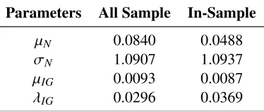
Table 1.1: Parameters of normal and inverse Gaussian distributions for standardized returns and volatility.
Parameters All Sample In-Sample
µN 0.0840 0.0488
σN 1.0907 1.0937
µIG 0.0093 0.0087
λIG 0.0296 0.0369
The first column corresponds to the in-sample period, while the second to the whole sample. µIG is a scale
parameter for the unconditional inverse Gaussian (IG) distribution of realized volatility.
Combining Equations (1.20) and (1.21), the conditional distribution of returns becomes
a normal-inverse Gaussian distribution (NIG) with the probability density function
com-puted as:
pd f(rt+1|It)=
Z
Yt+1
pd f(rt+1|Yt+1,It)· pd f(Yt+1|It) dYt+1
rt+1|It ∼ NIG(µN, σN, σt+1, αIG).
(1.23)
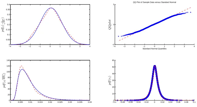
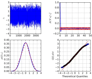
The NIG distribution provides a relatively accurate fit of the unconditional distribution
of returns. The first three graphs in Figure 1.1 demonstrate the very close match between
parametric and non-parametric unconditional distributions of standardized returns and
re-alized volatility, respectively. Table 1.1 shows the corresponding parameters of normal and
inverse Gaussian distributions.
Having the distributional assumption for returns, Theorem 1.2.1 demonstrates how to
obtain the approximated closed form expression for the multiple-step ahead forecast of the
realized volatility.
Figure 1.1: Comparison of parametric and non-parametric distributions of standardized returns, realized volatility and returns
−4 −3 −2 −1 0 1 2 3 4 0 0.05 0.1 0.15 0.2 0.25 0.3 0.35 0.4 p dfL ( rt √ R Vt )
0 0.005 0.01 0.015 0.02 0.025 0.03 0.035 0.04 0 20 40 60 80 100 120 140 p df ( √ R Vt )
−0.1 −0.08 −0.06 −0.04 −0.02 0 0.02 0.04 0.06 0.08 0.1 0 10 20 30 40 50 60 p df ( rt )
−4 −3 −2 −1 0 1 2 3 4 −5
0 5
Standard Normal Quantiles
Q
Q
p
lo
t
QQ Plot of Sample Data versus Standard Normal
Comparison of parametric (solid blue line) and non-parametric kernel distributions (red dashed line) of dardized returns, realized volatility and returns. The first graph compares the normal distribution of stan-dardized returns with the non-parametric distribution, while the second plots the corresponding QQ plot. The third graph illustrates the comparison between the IG distribution and the non-parametric distribution for realized volatility. The final graph shows the normal-inverse Gaussian (NIG) distribution for returns and the corresponding non-parametric distribution.
the NIG distribution with the conditional probability density function defined in(1.23), and
rt+h−1(h≥ 2) are independent of1,...,t+h−2. Then, the approximated h-step-ahead forecast
(h≥2) is obtained as follows:
ˆ
Yt(h)= E[Yt+h|It]≈ c1πt+c2(1−πt)+
βd
1πt +βd2(1−πt)
ˆ
Yt(h−1)+
+ βw
1πt+βw2(1−πt)Yˆtw(h−1)+ β m
1πt +βm2(1−πt)Yˆtm(h−1),
where:
πt = Pr[rt+1 < τ|It]=
Z τ
−∞
pd f(rt+1|It)drt+1
θ=
c1, βd1, β
w
1, β
m
1,c2, βd2, β
w
2, β
m
2
0
ˆ
Ytw(h−1)=
"ˆ
Yt(h−1)+...+Yˆt(h−5)
5
#
ˆ
Ytm(h−1)=
"ˆ
Yt(h−1)+...+Yˆt(h−22)
22
#
,
(1.25)
Proof See Appendix A.2.
In essence, Formula (1.24) is similar to the multiple-step-ahead forecast of the
GJR-GARCH(1,1) model — see Appendix A.1 for details. However, the TAR model has an
additional flexibility, since probabilityπtis time varying, while GJR-GARCH assumes that
the corresponding probability equals to 0.5. To facilitate comparison between these two
models, we compute the unconditional probability of a high volatility regime occurring
based on the NIG distribution (1.23) and from returns data. Here, the probability equals the
frequency of returns occurring, which is lower than the threshold value. The results show
a close match between these two methods: 11.3% (NIG)vs. 13.2% (historical returns) for
in-sample data.
Finally, we describe the multiple-step-ahead forecast using the rolling window
ap-proach. First, the parameters of the model are estimated using in-sample data, and
probabil-ityπtis computed. Second, multiple-step-ahead forecasts for the TAR model are calculated
based on Expression (1.24), whileπt remains constant. Probabilityπt can be computed for
each step of forecast, as well, but this will add additional computational burden, while the
and GJR-GARCH(1,1) models based on the formulas presented in Appendix A.1. Finally,
the rolling window is moved by one period ahead; the first observation is dropped, and the
parameters of the model, includingπt+1, are re-estimated.
1.3
Empirical Analysis
1.3.1
Data
The empirical analysis is based on high-frequency data for the S&P 500 index obtained
through the Realized Library of Oxford-Man Institute of Quantitative Finance (Library
Version 0.2), which is freely available:
“Researchers may use this library freely without restrictions so long as they quote in any
work which uses it: Heber, Gerd, Asger Lunde, Neil Shephard and Kevin Sheppard (2009)
“Oxford-Man Institute’s realized library”, Oxford-Man Institute, University of Oxford.”
The sample covers the period from 3 January of 2000 to 12 June of 2014, overall 3603
trading days. We exclude all days from the sample when the market was closed. Heber et al.
(2009) have created the Realized Library database, which provides daily data for about 11
realized measures for 21 assets. The authors clean the raw data obtained through Reuters
Data Scope Tick History and compute high-frequency estimators from cleaned data. We
use a realized kernel Barndorff-Nielsen et al. (2008) as a proxy for integrated variance.
1.3.2
Preliminary Data Analysis
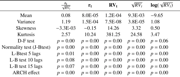
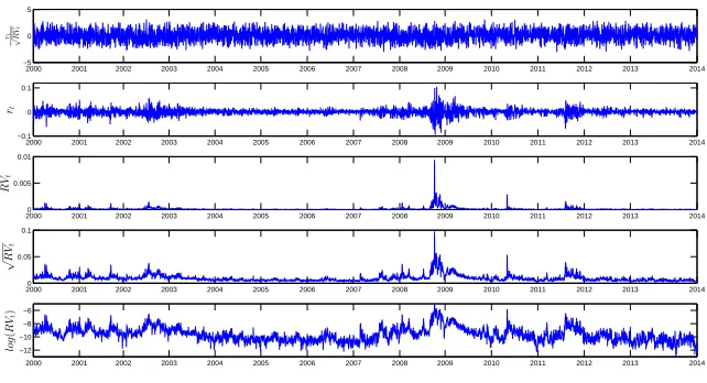
We start with data analysis of five main time series of interest: standardized returns,
Table 1.2: Descriptive statistics
rt
√
RVt rt RVt
√
RVt log(
√ RVt)
Mean 0.08 8.0E-05 1.2E-04 9.3E-03 −9.65 Variance 1.19 1.5E-04 7.5E-08 3.8E-05 1.08 Skewness −3.3E-03 −0.15 14.26 3.32 0.50 Kurtosis 2.57 10.24 381.25 24.58 3.47 D-F test p=0.00 p=0.00 p=0.00 p=0.00 p=0.06 Normality test (J-Btest) p=0.00 p=0.00 p=0.00 p=0.00 p=0.00 L-Btest 5 lags p=0.01 p=0.00 p=0.00 p=0.00 p=0.00 L-B test 10 lags p=0.08 p=0.00 p=0.00 p=0.00 p=0.00 L-B test 15 lags p=0.07 p=0.00 p=0.00 p=0.00 p=0.00 ARCH effect p=0.00 p=0.00 p=0.00 p=0.00 p=0.00
First four rows show unconditional sample mean, standard deviation, skewness and kurtosis of daily stan-dardized returns, returns, realized variance, realized volatility and the logarithm of the realized variance of the S&P500 index. Remaining rows depict p-values obtained from Dickey-Fuller, JarqueBera, LjungBox and Engle ARCH tests for these series.
presents the descriptive statistics, while Figure 1.2 illustrates the time series dynamics of
these variables.
Four of the variables are stationary at 5% according to the augmented Dickey–Fuller
test, whilelog(√RVt) is stationary at 6%. The recent financial crises and European sovereign
debt turmoil affected the volatility pattern and led to several spikes in the realized variance
series. Although these spikes look less pronounced in the logarithm of realized variance,
they remain very distinct from the volatility behaviour observed during calm times. This
observation motivates the introduction of the regime switching model for volatility process.
Daily returns are weakly correlated and follow a leptokurtic and negative skewed
distri-bution. By contrast, the distribution of the standardized returns is much closer to Gaussian,
which is in line with previous empirical findings: Andersen et al. (2001, 2010). Figure 1.3
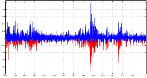
Figure 1.2: Time series dynamics of daily standardized returns, returns, realized variance, realized volatility and the logarithm of the realized variance
2000 2001 2002 2003 2004 2005 2006 2007 2008 2009 2010 2011 2012 2013 2014 −5
0 5
r
t
√
R
Vt
2000 2001 2002 2003 2004 2005 2006 2007 2008 2009 2010 2011 2012 2013 2014 −0.1
0 0.1
rt
20000 2001 2002 2003 2004 2005 2006 2007 2008 2009 2010 2011 2012 2013 2014 0.005
0.01
R
Vt
20000 2001 2002 2003 2004 2005 2006 2007 2008 2009 2010 2011 2012 2013 2014 0.05
0.1
√
R
Vt
2000 2001 2002 2003 2004 2005 2006 2007 2008 2009 2010 2011 2012 2013 2014 −12
−10 −8 −6
lo
g
(
R
Vt
)
Daily standardized returns, returns, realized variance, realized volatility and the logarithm of the realized variance of the S&P500 index. The sample period goes from January 2000 till June 2014 (3603 observations).
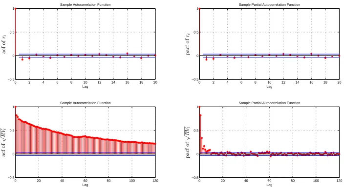
decays at a hyperbolic rate. This result is also consistent with the literature: Andersen et al.
(2003), Corsi et al. (2008), Choi et al. (2010).
1.3.3
Benchmark HAR Model
We start with the estimation of the benchmark linear Model (4) for the three specifications
of dependent variable RV, √RV and log(√RV), correspondingly. Table 1.3 presents the estimation results with the standard errors computed based on the HAC variance-covariance
matrix. Despite relatively highR2 for √RV andlog(√RV), the benchmark model fails to model spikes in volatility during turbulent times on financial markets. Figure 1.4 illustrates
this point and depicts a comparison between the in-sample forecast and the actual realized
Figure 1.3: Sample autocorrelations and partial autocorrelations of returns and real-ized volatility
0 2 4 6 8 10 12 14 16 18 20
−0.5 0 0.5 1 Lag a cf o f rt
Sample Autocorrelation Function
0 2 4 6 8 10 12 14 16 18 20
−0.5 0 0.5 1 Lag p a cf o f rt
Sample Partial Autocorrelation Function
0 20 40 60 80 100 120
−0.5 0 0.5 1 Lag a cf o f √ R Vt
Sample Autocorrelation Function
0 20 40 60 80 100 120
−0.5 0 0.5 1 Lag p a cf o f √ R Vt
Sample Partial Autocorrelation Function
Sample autocorrelations and partial autocorrelations of returns and realized volatility of the S&P500 index. The sample period goes from January 2000 till June 2014 (3603 observations).
Table 1.3: Heterogeneous autoregressive model (HAR) estimation
RVt √RVt log
√ RVt
Estimate SE Estimate SE Estimate SE
c 1.3E-05∗∗∗ 4.5E-06 4.6E-04∗∗∗ 2.0E-04 −0.44∗∗∗ 0.108
βd 0.223 0.146 0.395∗∗∗
0.058 0.336∗∗∗ 0.025
βw 0.461∗∗∗ 0.165 0.384∗∗∗ 0.081 0.440∗∗∗ 0.036
βm 0.216∗∗∗ 0.073 0.171∗∗∗ 0.048 0.178∗∗∗ 0.029
R2 50.4% 72.6% 73.2%
Reported are in-sample estimation results of the linear HAR model and corresponding standard errors com-puted based on the HAC variance-covariance matrix. The in-sample covers the period from February 2000 to
June 2014 (3582 observations). Here,∗∗∗means that the correspondingp-value is lower than 0.01.
In particular, benchmark Model (1.24) underestimates volatility by around 40% during
Figure 1.4: Comparison of actual realized volatility and model-implied volatility recovered from the HAR model
2000 2001 2002 2003 2004 2005 2006 2007 2008 2009 2010 2011 2012 2013 0
0.01 0.02 0.03 0.04 0.05 0.06 0.07 0.08 0.09 0.1
√
R
Vt
In-sample comparison of actual realized volatility (blue line) and volatility recovered from the HAR model (red line). The in-sample covers the period from February 2000 to June 2014 (3582 observations).
2010 and 2011. One of the explanations of the poor performance of the HAR model during
turbulent volatility periods is that it fails to take into account changes in volatility regimes.
Indeed, if volatility reacts to negative returns more than to positive returns, then the arrival
of the consequent negative shocks and volatility persistence can substantially increase the
future volatility level. On the other hand, different economic regimes might affect volatility
differently. We choose the TAR over SETAR model based on the higher value of the F12
statistics or, alternatively, the lower value of pbootstrapdefined in Subsection 1.2.2. 1
1.3.4
The TAR(2) Model
Next, we estimate the TAR(2) model (Table A.1 and Table 1.5), where past returns govern
changes in the volatility regimes.
Table A.1 shows that regression R2 improves substantially if regimes are driven by
past returns. As a result, high values of the F12 statistics lead to the rejection of the null
hypothesis (1.13) for all specifications at a 5% significance level. In addition, the optimal
value of the threshold parameter remains the same for two specifications: RVt and
√
RVt.
Theτthat corresponds to logarithm specification is closely related to the second threshold
of the TAR(3) model. However, the confidence interval for this parameter is very wide,
which leads to the imprecise estimate of the threshold parameter. Not surprisingly, this
model produces a less accurate one-step forecast than TAR(2). In particular, Dacco and
Satchell (1999) document that the imprecise estimate of the threshold parameter leads to
the poor forecasting performance of the simple switching model compared to the random
walk model. In both cases, changes in regimes are driven not only by negative returns
(leverage effect), but by significantly negative returns: −1.3% on a daily scale. McAleer and Medeiros (2008) also show that the transition between volatility regimes is governed
not by negative past returns, but by “very bad news” or very negative past returns.
The fact that changes in regimes are triggered by “very negative returns” can be
ex-plained by the volatility persistence and higher intensity of shocks during bad times.
Al-though the value of the threshold is not very large (it corresponds to the 11th percentile of
the returns distribution), the increasing number of negative returns can generate a spike in
the volatility. This explanation is similar to the option pricing literature, where researchers
modelled volatility by adding infinite activity jumps to the return’s process Ornthanalai
gener-Table 1.4: Comparison of the TAR(1) (or HAR) and TAR(2) models
RVt √RVt log(RVt)
R2of TAR(1) 50.4% 72.6% 73.2%
R2of TAR(2) 58.0% 74.9% 74.7%
τ −0.013 −0.013 0.001
l 0 0 0
F12 649.6 318.3 214.0
pbootstrap 0.00 0.03 0.00
Reported are sample estimation results of the linear HAR model and non-linear TAR(2) model. The
in-sample covers the period from February 2000 to June 2014 (3582 observations). pbootstrapis computed based
on 500 replications using the heteroscedastic bootstrap method. We set the maximum amount of lags equal to 10 in the TAR estimation.
ate a significant surge in volatility, high volatility persistence can lead to pronounced spikes
in the future volatility. Indeed, Figure 1.5 shows that the frequency of returns that are lower
than the threshold (red line) increased dramatically during recent financial crises. By
con-trast, returns that exceed the threshold (blue line) completely dominated “very negative
returns” during the period of low volatility in 2003–2007.
Table 1.5 shows that parameters βd, βw and βm are very different in high- and
low-volatility regimes. In particular, βw
1 is twice as large as the corresponding estimate in
the low-volatility regime for √RVt specification. Although some estimates have
nega-tive signs, they are not statistically significant at 10% for both realized volatility and
vari-ance models. By contrast, intercepts in both regimes are statistically negative for
log-arithmic specifications. Overall, corresponding estimates differ substantially in different
regimes, which highlights the importance of using the regime switching model. Next,
Fig-ure 1.6 shows that the 95% confidence interval for the threshold parameter is quite narrow
(τopt ∈[−0.014,−0.012]), although it includes two disjoints sets.
Finally, we compare the in-sample performance of the HAR and TAR(2) models for
Figure 1.5: The dynamics of returns in two regimes
2000 2001 2002 2003 2004 2005 2006 2007 2008 2009 2010 2011 2012 2013 2014 −0.1
−0.08 −0.06 −0.04 −0.02 0 0.02 0.04 0.06 0.08 0.1
rt
Daily returns in high (red line) and low (blue line) volatility regimes. The high (low) volatility regime occurs when the return is lower (higher) than the threshold. The sample period goes from February 2000 till June 2014 (3603 observations).
Figure 1.6: The confidence interval of threshold parameter
−0.0150 −0.01 −0.005 0 0.005 0.01 0.015
20 40 60 80 100 120 140 160 180
L
R
Threshold
Ninety five percent confidence interval for the threshold parameter of the TAR(2) model with √RVt
Table 1.5: TAR(2) estimation
RVt
√
RVt log
√ RVt
Estimate SE Estimate SE Estimate SE
c1 −2.6E-06 4.1E-05 −9.3E-05 9.5E-04 −0.321∗∗∗ 0.138
βd
1 0.331
∗ 0.189 0.332∗∗∗ 0.085 0.347∗∗∗ 0.029
βw
1 1.091
∗∗∗ 0.372 0.811∗∗∗ 0.191 0.475∗∗∗ 0.045
βm
1 −0.138 0.275 −0.018 0.128 0.133
∗∗∗ 0.037
c2 2.1E-05∗∗∗ 5.6E-06 0.001∗∗∗ 1.8E-04 -0.515∗∗∗ 0.150
βd
2 0.182 0.156 0.340
∗∗∗ 0.067 0.220∗∗∗ 0.038
βw
2 0.260
∗ 0.139 0.317∗∗∗ 0.067 0.498∗∗∗ 0.050
βm
2 0.268
∗∗∗
0.097 0.204∗∗∗ 0.045 0.243∗∗∗ 0.041
τ −0.013 −0.013 0.001
l 0 0 0
R2 58.0% 74.9% 74.7%
Reported are in-sample estimation results of the non-linear TAR(2) model and corresponding standard errors computed based on the HAC variance-covariance matrix. The in-sample covers the period from February 2000 to June 2014 (3582 observations). The first four rows correspond to the high-volatility, while the last
four rows correspond the low-volatility regime, respectively. Here,∗∗∗ and∗ mean that the corresponding
p-values are lower than 0.01 and 0.1, respectively.
DAX (Germany) and IPC Mexico (Mexico). The main findings remain robust to the
dif-ferent sets of indices: the non-linear model with an exogenous trigger is preferred over the
corresponding specification with the endogenous variable.
1.4
Forecast
In this section, we discuss one- and multiple-step-ahead forecasts of realized volatility
based on the TAR(2) model and several competing benchmarks. We assess their forecasting
Table 1.6: One-day-ahead out-of-sample forecast
January 2008 to January 2009 July 2011 to December 2011 January 2008 to June 2014
T AR HAR GARCH GJR T AR HAR GARCH GJR T AR HAR GARCH GJR RMS E 7.0 0.96 0.78 0.85 4.9 0.96 0.72 0.73 3.8 0.98 0.77 0.82
MAE 4.1 0.97 0.67 0.76 3.6 0.95 0.63 0.66 2.3 0.99 0.67 0.71
R2 0.70 0.68 0.56 0.64 0.42 0.38 0.24 0.39 0.75 0.74 0.66 0.70
pGW NA 0.54 0.00 0.00 NA 0.12 0.00 0.00 NA 0.71 0.00 0.00
The first four columns correspond to the period of recent financial crises in the U.S. from January 2008 to January 2009 (247 observations). The next four columns correspond to Eurozone crises from July 2011 to December 2011 (123 observations). The last four columns correspond to the period from January 2008 to June 2014 (1614 observations). The performance metrics are root mean square error (RMSE), mean absolute
error (MAE), theR2 of the Mincer–Zarnowitz regression and the p-value of the Giacomini and White test
based on the MAE metric. Two forecasts are identical in population under the null hypothesis, while TAR beats its competitors under the alternative. We compare TAR against all other models, while NA corresponds
to the TARvs. TAR case. The TAR column represents the actual value of RMSE and MAE errors, while the
HAR, GARCH and GJR columns, corresponding to the RMSE and MAE rows, equal the ratio of the TAR model to the following benchmark. Thus, a number below one indicates the improvement of the TAR model over its competitor. Observations for RMSE and MAE of the TAR model are standardized by 1000.
1.4.1
One-Day-Ahead Forecast
We start with the one-day-ahead forecast of the realized volatility, which is measured as
the square root of the realized kernel. The in-sample period covers 1968 days from
Jan-uary 2000 to JanJan-uary 2008. In addition to the HAR model, we choose several GARCH
specifications as benchmarks, including symmetric GARCH(1,1) and asymmetric
GJR-GARCH(1,1). Hansen and Lunde (2005) show that it is extremely hard to outperform a
simple GARCH (1,1) model in terms of forecasting ability. Meanwhile, TAR(2) is a
non-linear model; therefore, we need to add asymmetric GARCH specification to guarantee a
“fair” model comparison. Figure 1.7 and Table 1.6 assess the forecasting performance of
high- and low-frequency models.2
Next, we investigate whether the TAR forecast remains superior in population or not
2Although realized volatility ignores overnight returns, the superior performance of the high-frequency
Figure 1.7: One-step-ahead forecast in 2008-2014
20080 2009 2010 2011 2012 2013
0.02 0.04 0.06 0.08 0.1
T AR
20080 2009 2010 2011 2012 2013
0.02 0.04 0.06 0.08 0.1
HAR
20080 2009 2010 2011 2012 2013
0.02 0.04 0.06 0.08 0.1
GARCH
20080 2009 2010 2011 2012 2013
0.02 0.04 0.06 0.08 0.1
GJ R−GARCH
Comparison of actual and one-day-ahead forecasts based on the TAR(2), HAR, GARCH(1,1) and GJR-GARCH(1,1) models from January 2008 to June 2014 (1614 observations). The red line indicates the one-step forecast, while the blue line the actual data.
using the Giacomini and White test. Recall that the GW test is designed for the situation
where in-sample size is fixed, while out-of-sample size is growing. Thus, we assess the
forecasting performance of different models using the GW test only for the period from
January 2008 to June 2014 and not for U.S. and Eurozone financial crises. In the latter
cases, the GW test is likely to perform poorly, since we have a relatively short period of
sample periods: 247 and 123 observations, correspondingly.
The main results of this comparison are the following. First, high-frequency
mod-els significantly outperform lower frequency symmetric (GARCH) or asymmetric
(GJR-GARCH) daily models. This result highlights the importance of more accurate volatility
measuring based on the intra-daily data. Second, non-linear TAR(2) specification
according to the first three metrics. Surprisingly, TAR(2) does not outperform the HAR
model according to the GW test.
Finally, we assess the performance of volatility forecasts during times of financial
tur-moil: the U.S. financial crises in 2008 and the Eurozone crises in 2011. Although
high-frequency models continue to dominate GARCH specifications, the benefits of using the
non-linear TAR(2) model become substantial compared to linear specification: the latter’s
MAE is higher by 3% (U.S. crises) and 6% (Eurozone crises). By contrast, the MAE of the
HAR model is only 1% higher during the whole out-of-sample period. Figure 1.8 shows
that TAR(2) better captures spikes in volatility than linear specification during the recent
U.S. financial crises. Finally, both RMSE and MAE are lower for Eurozone crises and
whole out-of-sample periods compared with recent U.S. financial crises, which reflects the
learning process of the model, where recent volatility spikes help to improve the models’
performance.
To sum up, the benefits of using the non-linear TAR(2) model are most evident during
periods of elevated volatility. In addition, the model is able to predict spikes in
volatil-ity, even when we use a relatively calm period for in-sample estimation, since changes
in regimes are driven by moderately low returns. As a result, we do not rely on extreme
market events to forecast volatility.
1.4.2
Multiple-Step-Ahead Forecast
This section describes multiple-step-ahead forecasts for aggregate volatility. Specifically,
the object of interests is theh-step forecast of aggregate realized volatility
h
P
i=1
Yt+j|t. Table
1.7 compares TAR(2) and other benchmark models during recent U.S. financial crises,
Figure 1.8: One-step-ahead forecast in 2008-2009
2008 2009
0 0.01 0.02 0.03 0.04 0.05 0.06 0.07 0.08 0.09 0.1
T ARvsHAR
Comparison of actual and one-day-ahead forecasts based on the TAR(2) and HAR models during U.S. fi-nancial crises from January 2008 to January 2009 (247 observations). Red and green lines indicate one-step forecasts based on the TAR(2) and HAR models, correspondingly, while the blue line the actual data.
forecasts for all models.
The main findings remain similar to the one-step-ahead forecasts. First, high-frequency
models continue to dominate daily models at the five and 10 days’ ahead forecast.
Sec-ond, TAR(2) performs better than the linear HAR model according to RMSE, MAE and
R2. More importantly, the non-linear model outperforms linear specification, not only in
a particular sample, but also in population: we reject the null hypothesis of the GW test
that two forecast are identical at the 5% significance level. We based our conclusion on
the results of the GW test for the 2008–2014 years to take into account the growing size
of the out-of-sample dataset, as discussed in the Section 1.2.3. The GW test is based on
the MAE metric. In addition, the U.S. financial crises have substantially higher RMSE
and MAE compared with other periods, since periods of elevated volatility allow one to
Table 1.7: Multiple-days-ahead out-of-sample forecast
January 2008 to January 2009 July 2011 to December 2011 January 2008 to June 2014
T AR HAR GARCH GJR T AR HAR GARCH GJR T AR HAR GARCH GJR
5-days-ahead forecast
RMS E 33.5 0.98 0.56 0.55 23.1 0.99 0.60 0.59 17.3 0.99 0.53 0.55
MAE 22.2 0.98 0.49 0.47 14.5 0.96 0.46 0.45 10.1 0.98 0.43 0.44
R2 0.67 0.67 0.61 0.64 0.27 0.26 0.16 0.20 0.76 0.75 0.71 0.75
pGW NA 0.13 0.00 0.00 NA 0.06 0.00 0.00 NA 0.03 0.00 0.00
10-days-ahead forecast
RMS E 69.2 0.98 0.48 0.48 47.6 0.98 0.50 0.50 35.2 0.98 0.44 0.45
MAE 47.0 0.97 0.41 0.40 30.6 0.96 0.36 0.35 20.6 0.97 0.33 0.33
R2 0.63 0.63 0.61 0.61 0.15 0.15 0.16 0.14 0.73 0.73 0.71 0.74
pGW NA 0.21 0.00 0.00 NA 0.31 0.00 0.00 NA 0.01 0.00 0.00
The first four columns correspond to the period of recent financial crises in the U.S. from January 2008 to January 2009 (247 observations). The next four columns correspond to Eurozone crises from July 2011 to December 2011 (123 observations). The last four columns correspond to the period from January 2008 to June 2014 (1604 observations). The performance metrics are the root mean square error (RMSE), mean
absolute error (MAE), theR2of the Mincer–Zarnowitz regression and thep-value of the Giacomini and White
test based on the MAE metric. Two forecasts are identical in population under the null hypothesis, while TAR beats its competitors under the alternative. The TAR column represents the actual value of RMSE and MAE errors, while the HAR, GARCH and GJR columns, corresponding to the RMSE and MAE rows, equal the ratio of TAR model to the following benchmark. Thus, a number below one indicates the improvement of the TAR model over its competitor. Observations for RMSE and MAE of the TAR model are standardized by 1000. Finally, the first four rows correspond to the 5-step-ahead, while the next four to the 10-step-ahead forecast, respectively. Observations from RMSE and MAE are standardized by 1000.
Finally, we compare TAR(2) and its competitors during recent financial crisis. The
improvement in the MAE and RMSE metrics is comparable for crisis and longer
out-of-sample periods and equal to approximately 2%. Although the GW test indicates that the
TAR(2) and HAR model have the same forecasting errors, this can be explained by the
relatively short size of the out-of-sample for both U.S. and Eurozone crises.
To sum up, our non-linear model outperforms its competitors thanks to its ability to
capture different regimes in volatility and to measure volatility much more accurately than
daily models. In addition, our model achieves approximately the same rate of
improve-ment over the HAR model as much more complicated non-liner models, but with lower
computational costs, since the TAR(2) model has only two regimes. For example, Scharth
im-Figure 1.9: Multiple-step-ahead forecast in 2008-2014
20080 2009 2010 2011 2012 2013
0.05 0.1 0.15 0.2 0.25 0.3 0.35
T AR
20080 2009 2010 2011 2012 2013
0.05 0.1 0.15 0.2 0.25 0.3 0.35
HAR
20080 2009 2010 2011 2012 2013
0.05 0.1 0.15 0.2 0.25 0.3 0.35
GARCH
20080 2009 2010 2011 2012 2013
0.05 0.1 0.15 0.2 0.25 0.3 0.35
GJ R−GARCH
Comparison of aggregate volatility over five days and corresponding forecasts based on the TAR(2), HAR, GARCH(1,1) and GJR-GARCH(1,1) models from January 2008 to June 2014 (1604 observations). The red line indicates the aggregate five-step forecast, while the blue line the actual data.
provement in forecasting performance over the HAR model of around 3%. This feature is
essential for practical applications.
1.5
Conclusions
This chapter develops a non-linear threshold model for RV (realized volatility), allowing
us to obtain a more accurate volatility forecast, especially during periods of financial crisis.
The changes in volatility regimes are driven by negative past returns, where the threshold
equals approximately −1%. This finding remains robust to different functional forms of volatility and different set of indices from both developing and developed countries. The