Thermoelasticity of Hexagonal Close-Packed Iron from the Phonon Density of States

(1)

Iron from the Phonon Density of States

Thesis by

Caitlin A. Murphy

In Partial Fulfillment of the Requirements

for the Degree of

Doctor of Philosophy

CALIFORNIA INSTITUTE OF TECHNOLOGY

Pasadena, California

2012

(2)

 2012

Caitlin A. Murphy

(3)

Acknowledgements

First and foremost, I would like to thank my advisor, Jennifer Jackson. Our research

discussions provided me with a solid foundation in mineral physics, from both Earth

Science and Materials Science perspectives. In addition, I benefitted greatly from your

novel and interesting approaches to the unanswered questions about the deep Earth.

Equally important are the more personal aspects of your mentorship; your annual lab

parties, outings to the Rathskeller, and friendship contributed greatly to my experience as a

graduate student. Finally, mineral physics at Caltech would not be the same without such

wonderful puns (intended or not) as the need to have “all of our DACs in a row” before

heading to the synchrotron.

I am especially thankful for the incredible research opportunities afforded to me

over the past five years, and the people who made them possible. In addition to Jennifer, I

would like to thank the other members of the self-proclaimed “beam team”: Wolfgang

Sturhahn, Bin Chen, and Dongzhou Zhang. The quality of the experimental data on which

this thesis is based—in addition to the corresponding analyses—would not have been

possible without Wolfgang’s expertise and guidance. In addition, I benefitted greatly from

research discussions with Bin and Dongzhou, related to both experimental techniques and

(4)

inspirational, and it was an honor to perform our experiments together. Finally, I thank the

past and present members of the Inelastic and Nuclear Resonant Scattering group at the

Advanced Photon Source, Argonne National Laboratory, for your excellent beamline and

constant support of our experiments: Jiyong Zhao, Michael Hu, Tom Toellner, Esen Alp,

Hassan Yavas, Ayman Said, and Ahmet Alatas. A special thank you goes to Tom Toellner

for your helpful discussions about both my experiments and career goals.

I thank the faculty at Caltech for providing me with a strong foundation in the

underlying principles and applications of Mineral Physics. I thank Paul Asimow for sharing

your seemingly endless knowledge of geochemistry, and in particular for your insights on

chemical thermodynamics, differentiation of the Earth, and isotope fractionation. I also

thank Brent Fultz for allowing me to see our experiments and results through the eyes of a

Materials Scientist, both in your course on phase transformations and at your group

meetings. Finally, thank you both for serving on my thesis committee; this thesis has

benefitted greatly from your diverse expertise and invaluable feedback.

I would also like to thank Rob Clayton, first for serving on my thesis committee. In

addition, thank you for three great years as a Teaching Assistant on the Ge111 field trips to

the Salton Sea. The field experience, in-depth exposure to applied geophysics techniques,

and teaching experience I gained from those trips are invaluable. Your efficiency in the

field, passion for teaching, and dedication to the students are all exemplary qualities.

Finally, thank you for your support and guidance, especially during my first years at

Caltech; with only a few words, you had an incredible impact on my experience here.

I thank Tom Heaton for imparting on me your vast knowledge of seismology from

(5)

foundation in the principles of seismology and the more relevant features of seismometers

and seismic data analysis. I also thank you for your passion for teaching and the students,

which is evident in everything you do. I am grateful for your friendship during my final

years at Caltech, and for your stories about the Seismolab, geophysics, and life in general.

I am very grateful that I got to explore a proposition project with Professor George

Rossman, investigating the coloration mechanism of beryllium-doped corundum with the

electron paramagnetic resonance technique. Your enthusiasm for the project was truly

contagious, and your mentoring during my first year was invaluable. I continue to be awed

by the wealth of information I learned from you after just one short year, and I look

forward to writing up that project with you soon.

I thank my officemates—Ting Chen, Laura Alisic, Jeff Thompson, Semechah Liu,

and Yiran Ma—for providing such a positive and comfortable work environment. In

addition, I am thankful for the wonderful support staff in the Seismolab: Viola Carter,

Evelina Cui, Sarah Gordon, Rosemary Miller, Donna Mireles, and Julia Zuckerman. I

appreciate the efficiency and care with which you handle Siesmolab affairs, and my

day-to-day experience would not have been the same without your smiling faces. Thank you for

fostering a fun and friendly environment via the Seismo Socials and Annual Retreat.

I had the privilege of attending two incredible enrichment trips during my time at

Caltech. First, I thank John Eiler and Jean-Philippe Avouac for organizing the Enrichment

Trip to the Alps, and our local hosts—Lukas Baumgartner, David Flöss, Robert Bodner—

for sharing their extensive knowledge about Alpine geology and the wonderful culture

embedded in the Swiss and Italian Alps. In addition, I thank Jason Saleeby and John Eiler

(6)

the Hawaiian geology and culture made for a truly memorable trip.

My experience at Caltech has also been enriched by extracurricular activities and

the wonderful friends I have made. I would like to thank the Love Waves for four amazing

softball seasons, each with just enough wins to keep morale high. I thank Jack Prater,

Kathy Torres and the rest of the Caltech volleyball community for providing me with a fun

way to blow off steam. And I am grateful to my friends across the Institute for all of the

great memories: Lisa Mauger, Steve Skinner, Jessica Pfeilsticker, Keenan Crane, Patrick

Sanan, Mike Deceglie, Emily Warren, and Karín Menéndez-Delmestre.

I thank my family for your unending support during my time in graduate school.

Your frequent presence helped make Southern California feel like home, and I am so

grateful that you were there through all of the major milestones.

Finally, I thank my husband, Don Jenket. I cannot believe it has already been five

years since we left Quantico for the West Coast, and the incredible journey we have had

since. My weekend trips to Oceanside helped me to accelerate and succeed in my graduate

program, as they motivated me to push hard during the week so I could enjoy our few days

together over the weekend. Our trips to New Zealand, Italy, and the Canadian Rockies were

wonderful rewards for all of our hard work. And your experience in the Marines helped me

to keep the proper perspective about graduate school and life in general. I greatly

appreciate all you have done to support me during graduate school, and I am excited to start

(7)

Abstract

Iron is the main constituent in Earth’s core, along with ~5 to 10 wt% Ni and some

light elements (e.g., H, C, O, Si, S). This thesis explores the vibrational thermodynamic and

thermoelastic properties of pure hexagonal close-packed iron (ε-Fe), in an effort to improve

our understanding of the properties of a significant fraction of this remote region of the

deep Earth and in turn, better constrain its composition.

In order to access the vibrational properties of pure ε-Fe, we directly probed its total

phonon density of states (DOS) by performing nuclear resonant inelastic x-ray scattering

(NRIXS) and in situ x-ray diffraction (XRD) experiments at Sector 3-ID-B of the

Advanced Photon Source (APS) at Argonne National Laboratory. NRIXS and in situ XRD

were collected over the course of ~14 days at eleven compression points between 30 and

171 GPa, and at 300 K. Our in situ XRD measurements probed the sample volume at each

compression point, and our long NRIXS data-collection times and high-energy resolution

resulted in the highest statistical quality dataset of this type for ε-Fe to outer core pressures.

Hydrostatic conditions were achieved in the sample chamber for our experiments at smaller

compressions (P ≤ 69 GPa) via the loading of a neon pressure transmitting medium at the

GeoSoilEnviroCARS (GSECARS) sector of the APS. For measurements made at P > 69

(8)

transmitting medium.

From each measured phonon DOS and thermodynamic definitions, we determined

a wide range of vibrational thermodynamic and thermoelastic parameters, including the

Lamb-Mössbauer factor; vibrational components of the specific heat capacity, free energy,

entropy, internal energy, and kinetic energy; and the Debye sound velocity. Together with

our in situ measured volumes, the shape of the total phonon DOS and these parameters

gave rise to a number of important properties for ε-Fe at Earth’s core conditions.

For example, we determined the Debye sound velocity (vD) at each of our

compression points from the low-energy region of the phonon DOS and our in situ

measured volumes. In turn, vD is related to the compressional and shear sound velocities via

our determined densities and the adiabatic bulk modulus. Our high-statistical quality

dataset places a new tight constraint on the density dependence of ε-Fe’s sound velocities

to outer core pressures. Via comparison with existing data for iron alloys, we investigate

how nickel and candidate light elements for the core affect the thermoelastic properties of

iron. In addition, we explore the effects of temperature on ε-Fe’s sound velocities by

applying pressure- and temperature-dependent elastic moduli from theoretical calculations

to a finite-strain model. Such models allow for direct comparisons with one-dimensional

seismic models of Earth’s solid inner core (e.g., the Preliminary Reference Earth Model).

Next, the volume dependence of the vibrational free energy is directly related to the

vibrational thermal pressure, which we combine with previously reported theoretical values

for the electronic and anharmonic thermal pressures to find the total thermal pressure of

ε-Fe. In addition, we found a steady increase in the Lamb-Mössbauer factor with

(9)

This behavior is related to the high-pressure melting behavior of ε-Fe via Gilvarry’s

reformulation of Lindemann’s melting criterion, which we used to obtain the shape of

ε-Fe’s melting curve up to 171 GPa. By anchoring our melting curve shape with

experimentally determined melting points and considering thermal pressure and

anharmonic effects, we investigated ε-Fe’s melting temperature at the pressure of the

inner–core boundary (ICB, P = 330 GPa), where Earth’s solid inner core and liquid outer

core are in contact. Then, combining this temperature constraint with our thermal pressure, we determined the density of ε-Fe under ICB conditions, which offers information about

the composition of Earth’s core via the seismically inferred density at the ICB.

In addition, the shape of the phonon DOS remained similar at all compression

points, while the maximum (cutoff) energy increased regularly with decreasing volume. As

a result, we were able to describe the volume dependence of ε-Fe’s total phonon DOS with

a generalized scaling law and, in turn, constrain the ambient temperature vibrational

Grüneisen parameter. We also used the volume dependence of our previously mentioned vD

to determine the commonly discussed Debye Grüneisen parameter, which we found to be

~10% smaller than our vibrational Grüneisen parameter at any given volume. Finally,

applying our determined vibrational Grüneisen parameter to a Mie-Grüneisen type

relationship and an approximate form of the empirical Lindemann melting criterion, we

predict the vibrational thermal pressure and estimate the high-pressure melting behavior of ε-Fe at Earth’s core pressures, which can be directly compared with our previous results.

Finally, we use our measured vibrational kinetic energy and entropy to approximate ε-Fe’s vibrational thermodynamic properties to outer core pressures. In particular, the

(10)

isotopic partition function ratios of ε-Fe and in turn, provide information about the

partitioning behavior of solid iron in equilibrium processes. In addition, the volume

dependence of vibrational entropy is directly related to the product of ε-Fe’s vibrational

component of the thermal expansion coefficient and the isothermal bulk modulus, which

we find to be independent of pressure (volume) at 300 K. In turn, this product gives rise to

the volume-dependent thermal expansion coefficient of ε-Fe at 300 K via established EOS

parameters, and the vibrational Grüneisen parameter and temperature dependence of the

(11)

List of Figures

1.1. Cut-out model of the Earth ... 2

1.2. Average Earth models ... 3

1.3. Pressure–temperature phase diagram of iron ... 5

2.1. Panoramic Diamond-Anvil Cell (DAC) ... 17

2.2. Diamond mounting ... 18

2.3. Sample chamber ... 23

2.4. Sector 3-ID-B at the Advanced Photon Source ... 25

2.5. Example MAR3450 x-ray diffraction (XRD) image ... 27

2.6. Correlation of reported EOS parameter uncertainties ... 28

2.7. Schematic of NRIXS Theory ... 31

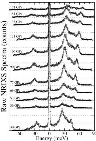
2.8. Our raw NRIXS spectra for ε-Fe ... 40

2.9. Our raw NRIXS spectra for ε-Fe, normalized ... 41

2.10. Example raw NRIXS spectrum with detail ... 42

2.11. Our measured phonon DOS for ε-Fe ... 46

3.1. Vibrational free energy per 57Fe atom at 300 K... 51

3.2. Vibrational thermal pressure of ε-Fe ... 54

(15)

3.4. High-pressure melting behavior of ε-Fe ... 60

4.1. Comparison of measured and scaled phonon DOS of ε-Fe ... 69

4.2. Scaling parameter analysis demonstration ... 71

4.3. Grüneisen parameters of ε-Fe ... 74

5.1. Lamb-Mössbauer factor of ε-Fe from NRIXS data ... 83

5.2. Vibrational kinetic energy of ε-Fe from NRIXS data ... 85

5.3. Reduced isotopic partition function ratios of ε-Fe ... 86

5.4. Vibrational entropy of ε-Fe ... 87

5.5. Vibrational thermal expansion coefficient of ε-Fe at 300 K ... 88

5.6. Our density-dependent sound velocities at 300 K ... 91

5.7. Debye sound velocities of ε-Fe at 300 K ... 94

5.8. Compressional sound velocities of ε-Fe at 300 K ... 94

5.9. Density dependence of our compressional and shear sound velocities of ε-Fe at 300 K with PREM ... 103

6.1. Debye sound velocities of ε-Fe and iron alloys ... 109

6.2. Compressional sound velocities of ε-Fe and iron alloys ... 110

6.3. Compressional sound velocities of ε-Fe and Fe3C ... 113

6.4. Density dependence of compressional sound velocities of ε-Fe and iron alloys ... 114

6.5. Shear sound velocities of ε-Fe and iron alloys ... 117

6.6. Density dependence of ε-Fe’s sound velocities from our finite-strain model at 300 K, with PREM ... 122

(16)

List of Tables

xvii.1. Acronyms for average Earth models and major boundaries in the

deep Earth ... vxii

xvii.2. Terms related to experimental techniques discussed in this thesis ... xviii

xvii.3. Variables that appear frequently in this thesis ... xix

2.1. Parameters from a reported EOS and our XRD data collection for ε-Fe ... 29

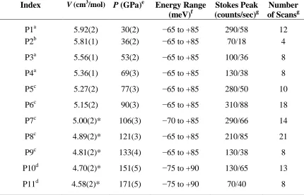
2.2. Pressures and experimental parameters for our NRIXS data collection ... 38

3.1. Free energy and Lamb-Mössbauer temperature from NRIXS data, and melting temperatures and thermal pressures from analysis ... 52

3.2. Anchor melting point parameters ... 62

4.1. Specific heat capacity, internal energy, and Debye sound velocity of ε-Fe from NRIXS data ... 75

5.1. Vibrational thermodynamic parameters of ε-Fe from the phonon DOS ... 92

5.2. Elasticity of ε-Fe from the phonon DOS ... 93

6.1. Input parameters for our finite-strain model ... 126

(17)

NOTATION AND NOMENCLATURE

As a reference, we provide descriptions and definitions for the following list of

acronyms and variables that appear frequently in the chapters of this thesis. The following

three tables are organized by related topics.

Table xvii.1. Acronyms for average Earth models and major boundaries in the deep Earth.

Acronym Definition and Description

CMB Core–mantle boundary: A seismically determined boundary between Earth’s iron-rich outer core and the overlying silicate-rich mantle, which lies at a depth of ~2891 km. It is indicated in seismic models by a sudden increase in density, decrease in compressional sound velocity, and disappearance of shear waves.

ICB Inner–core boundary: A seismically determined boundary between Earth’s solid inner core and liquid outer core, which lies at a depth of ~5150 km. It is indicated in seismic models by a slight increase in density and compressional sound velocity, and the reappearance of shear waves.

(18)

(19)

(20)

(21)

Variable Common

Units Description

γ -- Grüneisen parameter: the coefficient that relates a material’s internal energy and thermal pressure; subscripts indicate vibrational (γvib) or Debye (γD) Grüneisen parameters; the former

is related to the phonon density of states, and the latter is based on Debye’s approximate description of the same spectrum.

lnβ -- Reduced isotopic partition function ratio: the ratio of isotope ratios for a given material and for dissociated atoms at equilibrium; β-factors are related to the equilibrium fractionation factor and in turn, determine the distribution of isotopes in equilibrium processes.

α 10−5K−1 Thermal expansion coefficient: the change in volume that results from increasing temperature at constant pressure; subscripts indicate the vibrational contribution to the thermal expansion coefficient (αvib).

δT -- Anderson-Grüneisen parameter: the volume dependence of the

(22)

Chapter 1 Introduction

1.1 The Earth’s Core

The Earth’s core accounts for approximately one-sixth of the Earth’s volume and

one-third of its mass. We cannot directly sample such great depths in the Earth, so we rely

largely on seismology to probe this remote region. Seismic observations of Earth’s normal

modes provide constraints on the density of the deep Earth, and body-wave travel times are

related to the velocity at which compressional and shear sound waves travel through it.

Such observations have revealed that to first order, the Earth comprises four basic layers:

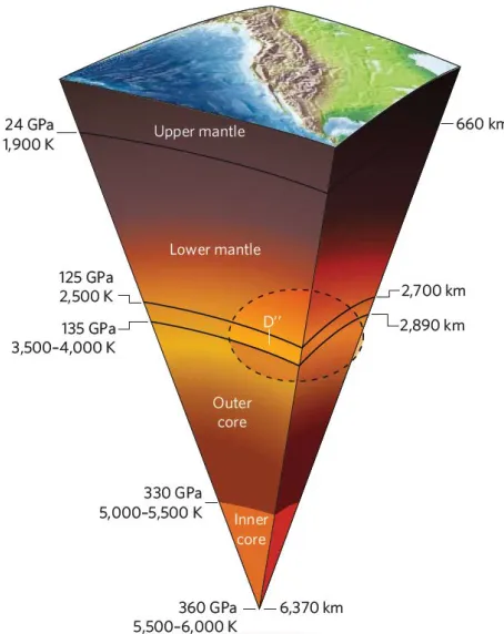
crust, mantle, outer core, and inner core (Figure 1.1). More specifically, the seismically

inferred sharp increase in density across the core–mantle boundary suggests that the Earth’s

core is compositionally distinct from the overlying mantle. In addition, it has been

determined that while Earth’s inner and outer cores are likely to be compositionally similar

based on their comparable densities, they have very different elastic properties. Shear

waves do not propagate through the outer core, but they reappear in the inner core, thus

implying that a liquid outer core surrounds the solid inner core. Further evidence for a

(23)

Figure 1.1. Cut-out model of the Earth. The four basic layers of Earth’s interior are the crust; the silicate-rich mantle, which is often divided further into an upper mantle (P < 24 GPa) and lower mantle (24 GPa < P < 135 GPa); the liquid metallic outer core (135 GPa < P < 330 GPa); and the solid metallic inner core (330 GPa < P < 364 GPa). We note that the pressure at the center of the Earth is mislabeled. Figure taken from Duffy (2008).

generated by the rotation and vigorous convection of an electrically conductive fluid (i.e.,

the iron-rich liquid outer core) deep in the Earth.

The combination and inversion of astronomic-geodetic data (e.g., radius, mass, and

moment of inertia) with observed free oscillations, long-period surface waves, and

body-wave travel times results in average Earth models. These models assume a radially

symmetric Earth (i.e., they are one-dimensional), and therefore they do not contain any

information about lateral variations of the Earth’s elastic properties. Instead, average Earth

models provide information about the average elastic properties of deep Earth materials, in

addition to estimates for the depths (pressures) of major boundaries that correspond to

discontinuities in the inferred elastic and structural properties.

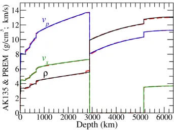
Two of the most commonly cited average Earth models are AK135 (Kennett et al.,

(24)

1981). There are slight differences between AK135 and PREM near the boundaries

between distinct layers in the deep Earth, but overall they agree on the general features

(Figure 1.2). For example, they place the core–mantle boundary (CMB) at a depth of

2891 km—which corresponds to a pressure of ~136 GPa—where there is a sudden increase

in density by 78%, a decrease in compressional wave velocity by 41%, and the complete

disappearance of shear waves. In addition, they find the boundary between the solid inner

core and the liquid outer core (inner–core boundary; ICB) to be at a depth of 5150 km

(329 GPa), based on the reappearance of shear seismic waves and smaller discontinuities

(25)

in the density (~5%) and compressional wave velocities (~6.5%) (e.g., Dziewonski and

Anderson, 1981). Finally, within a given layer, models like PREM and AK135 provide

radial density and velocity profiles (Figure 1.2), which are related to the composition of

these remote regions via comparison with theoretical and experimental investigations of the

structural and thermoelastic properties of candidate materials.

From arguments based on seismic observations, laboratory experiments, and

cosmochemical observations, iron is considered to be the main constituent in Earth’s core

(e.g., Birch, 1964; McDonough, 2003). We will return to a discussion of the more minor

constituents in the core in Section 1.3, but for now we focus on our current understanding

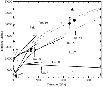
of the high-pressure properties of pure iron. Pure iron crystallizes in the body-centered

cubic (bcc; α-Fe) crystal structure at ambient pressure and temperature (PT) conditions. At

ambient pressure, iron transitions to the face-centered cubic structure (γ-Fe) at ~1185 K

(e.g., Birch, 1940), and then back to a bcc structure (δ-Fe) at ~1667 K before melting

around 1811 K (e.g., Strong et al., 1973) (Figure 1.3). At low temperatures, iron undergoes

a single phase transition to the more densely packed hexagonal close-packed structure (hcp; ε-Fe) around 10 to 18 GPa (e.g., Bancroft et al., 1956; Stixrude et al., 1994; Dewaele et al.,

2006; Sha and Cohen, 2006). Finally, the crystal structure at simultaneous high-pressure

and temperature conditions is somewhat controversial (e.g., Saxena and Dubrovinsky,

2000), but existing data suggest that ε-Fe is the stable phase at core condition (e.g., Vočadlo

et al., 2000; Alfè et al., 2001; Ma et al., 2004; Nguyen and Holmes, 2004; Tateno et al.,

2010). Therefore, firmly establishing the high-pressure material properties of ε-Fe—the

end-member composition of the core—with high-pressure experiments is essential for

(26)

Figure 1.3. Pressure–temperature phase diagram of iron. At ambient conditions, iron takes on the bcc structure (α); at low-P and high-T conditions, iron transforms first into an fcc structure (γ) and then back to a bcc structure (δ); at low-T and high-P conditions, iron transforms into an hcp structure (ε); the crystal structure of iron at high-PT conditions remains controversial, although there is significant evidence that ε-Fe remains stable throughout the PT conditions of Earth’s core (e.g., Tateno et al., 2010). Figure taken from Nguyen and Holmes (2004) and associated references within.

1.2 Investigating Iron at Earth’s Core Conditions

A wide variety of techniques have been used to investigate the structural, vibrational, and thermoelastic properties of ε-Fe. Shock-compression experiments have

historically been the preferred method for experimentally probing the properties of

candidate core materials, in part, because they simultaneously induce the pressure and

temperature conditions expected in Earth’s core (~136 to 364 GPa, T > 2500 K). In such

(27)

“flyer” that has been accelerated toward it using, e.g., a two-stage light gas gun. Across the

resulting shock front, iron undergoes a nearly discontinuous, adiabatic change of state,

from which one can investigate the pressure-volume-internal energy equation of state (e.g.,

McQueen et al., 1970), adiabatic bulk modulus (e.g., Jeanloz, 1979), compressional sound

velocity (e.g., Jeanloz, 1979; Brown and McQueen, 1986; Nguyen and Holmes, 2004), and

melting behavior (e.g., Brown and McQueen, 1986; Williams et al., 1987; Yoo et al., 1993;

Ahrens et al., 2002; Nguyen and Holmes, 2004) of ε-Fe at simultaneous high-pressure and

temperature (PT) conditions. For shocks that are large enough to induce melting of iron,

one can also probe the high-PT bulk sound velocity and Grüneisen parameter of the liquid

phase (e.g., Jeanloz, 1979; Brown and McQueen, 1986; Nguyen and Holmes, 2004).

The induced pressures, sample densities, and internal energies from

shock-compression experiments are very well-known via the measured shock velocity, particle

(sample) velocity, and initial pressure and density of the system, but it is difficult to

accurately determine the temperature of a given shock. For transparent materials, the shock

temperature can be measured fairly accurately (ΔT ~ 50 K at 4000 K) using time-resolved

optical pyrometry (e.g., Luo et al., 2004). Determining the shock temperature for an opaque

sample is much more challenging, so for experiments on ε-Fe, it is often approximated

from thermodynamic calculations that use estimated values for ε-Fe’s Grüneisen parameter

and heat capacity. Reported temperature uncertainties from this method are typically on the

order of ~500 K (e.g., Brown and McQueen, 1986; Nguyen and Holmes, 2004).

A complementary approach to investigating thermoelastic and thermodynamic

properties at core pressures is to use static compression in the diamond-anvil cell (DAC;

(28)

similar pressures as those produced with shock compression, but they are performed at

constant volume rather than constant entropy. In addition, the nature of static compression

allows for independent manipulation of pressure and temperature and, in turn, a more

controlled sampling of PT conditions. However, determining the pressure experienced by

the sample in a DAC is difficult, and reported pressures are often based on calibrated

pressure scales for secondary pressure markers that disagree significantly at core pressures

(e.g., Steinle-Neumann et al., 2001; Dorogokupets and Oganov, 2006). The recorded

pressure from a secondary pressure marker is also sensitive to the sample chamber

environment (i.e., degree of hydrostaticity), so additional uncertainties are introduced to

reported pressures based on the DAC preparations for a given experiment. For example, the

pressure experienced by the sample may be significantly different than that experienced by

the secondary pressure marker, which is most often not the sample itself.

A wide variety of DAC techniques have been used to investigate the high-pressure

structural and thermoelastic properties of iron. Synchrotron x-ray diffraction (XRD) has

been used to investigate the crystal structure and compressibility of ε-Fe, the combination

of which gives rise to its isothermal equation of state (e.g., Mao et al., 1990; Dewaele et al.,

2006). In addition, the use of a laser-heated DAC allows for the investigation of ε-Fe’s

thermal equation of state and melting behavior via high-PT XRD experiments

(Dubrovinsky et al., 1998; Shen et al., 1998; Uchida et al., 2001; Ma et al., 2004; Tateno et

al., 2010). High-pressure Raman spectroscopy has been used to measure ε-Fe’s E2g Raman

mode, which is correlated with a transverse acoustic phonon and, in turn, provides

information about its shear sound velocity (Merkel et al., 2000). Inelastic x-ray scattering

(29)

of x-rays by long-wavelength acoustic phonons (e.g., Antonangeli et al., 2004). In general,

IXS can be used to investigate the elastic constants and shear sound velocities of single crystals, but single crystals are not preserved across iron’s α→ε phase transition, and thus

are not available for ε-Fe. For IXS measurements on polycrystals, the shear mode is

extremely difficult to detect, typically because the background is too high or elastic

scattering dominates at low energies. Finally, nuclear resonant inelastic x-ray scattering

(NRIXS) is an especially powerful technique that probes the total phonon density of states

of select resonant isotopes and, in turn, their sound velocities and vibrational

thermodynamic properties. Somewhat fortuitously for the Earth Science community, 57Fe is

one such isotope, and therefore has been the focus of many high-pressure NRIXS studies

(e.g., Lübbers et al., 2000; Mao et al., 2001; Giefers et al., 2002; Lin et al., 2005; Mao et

al., 2008; Murphy et al., 2011b). NRIXS experiments of ε-Fe will be the focus of this

study, and will be described in more detail in Chapter 2.

Finally, many theoretical studies have been dedicated to investigating the structural,

thermoelastic, and thermodynamic properties of iron at core conditions. In particular, ab

initio techniques have been applied by a number of research groups to investigate the

Helmholtz free energy (F) and, in turn, the equation of state, thermodynamic, and

thermoelastic properties of ε-Fe (e.g., Wasserman et al., 1996; Stixrude et al., 1997; Alfè et

al., 2001; Vočadlo et al., 2009; Sha and Cohen, 2010a). From the volume dependence of F,

these studies explored the specific heat capacity, bulk modulus, thermal expansion

coefficient, and Grüneisen parameter of ε-Fe up to pressures of 400 GPa and temperatures

of 8000 K, often producing significantly different results at core conditions. Access to such

(30)

they have access to is much larger than that of most experiments. However, the utility of

theoretical studies at such conditions is limited by their lack of confirmation from

experimental results; in general, it is via benchmarking against experiments that the

accuracy of theoretical calculations is discussed.

Another important strength of theoretical calculations is their ability to probe

properties that are difficult or impossible to measure experimentally at in situ high-PT

conditions. For example, theoretical calculations provide the most complete information

about the pressure and temperature dependences of ε-Fe’s elastic moduli (e.g., Vočadlo et

al., 2009; Sha and Cohen, 2010a). In addition, they are currently the sole source of

information about electronic contributions to the thermodynamic and thermoelastic

properties of ε-Fe at high-PT conditions, since experimental techniques that probe the

electronic density of states require a free sample surface.

Despite the wealth of data provided by theoretical, shock-compression, and

static-compression experiments—and in part because of it—many of the properties of iron at the

PT conditions of Earth’s core remain highly uncertain. For example, there is an ongoing

debate about the crystal structure of iron at Earth’s core conditions; many studies support the stability of ε-Fe, but a variety of solid–solid phase transitions have been suggested as a

result of both static- and shock-compression experiments (e.g., Brown and McQueen, 1986;

Anderson and Isaak, 2000; Andrault et al., 2000; Dubrovinsky et al., 2000b; Saxena and

Dubrovinsky, 2000). In addition, even if we assume ε-Fe remains stable throughout Earth’s

core, there is significant disagreement between theoretical (e.g., Vočadlo et al., 1997; Sola

et al., 2009; Sha and Cohen, 2010a) and experimental (e.g., Brown and McQueen, 1982;

(31)

determinations of its equations of state (EOS). The ambient pressure volume (V0),

isothermal bulk modulus (KT0), and pressure derivative of the isothermal bulk modulus

(KT0′) from various static-compression experiments seem to be converging around V0 ~

6.75 cm3/mol, KT0~ 160 to 165 GPa, and KT0′ ~ 5.33 to 5.38 (e.g., Dewaele et al., 2006).

However, many theoretical calculations of ε-Fe’s EOS report dramatically different EOS

parameters: V0~ 6.08 cm3/mol, KT0~ 290 GPa, and KT0′ ~ 4 to 4.44 (e.g., Sha and Cohen,

2010a). Such discrepancies result in significantly different predicted pressures for a given

volume at small compressions (V V₀ ≥0.85) (Dewaele et al., 2006; Sha and Cohen, 2006),

and are due, in part, to the fact that theoretical calculations predict ε-Fe remains magnetic

until ~50 GPa. Another likely factor is the trade-off between KT0 and KT0' when fitting an

EOS to pressure–volume relationships measured with static-compression experiments.

Finally, we note that the predicted melting temperatures for ε-Fe at the pressure of

Earth’s inner–core boundary (330 GPa) span a range of almost 3000 K: from 4850 ± 200

K (Boehler, 1993) to 7600 ± 500 K (Williams et al., 1987). Many studies have found the melting temperature of ε-Fe falls in a slightly narrower range of ~5000 to 6000 K (e.g.,

Brown and McQueen, 1986; Shen et al., 1998; Laio et al., 2000; Ma et al., 2004; Nguyen

and Holmes, 2004; Murphy et al., 2011a; Jackson et al., 2012). However, recent reports

have predicted melting temperatures consistent with both the upper (Sola and Alfè, 2009)

and lower (Komabayashi and Fei, 2010) bounds of the original range, suggesting that we

are not yet converging on a single melting point for ε-Fe at Earth’s core conditions.

1.3 Alloying and Temperature Effects of Iron

Determining the properties of Earth’s core becomes even more complicated when

(32)

the overall composition. In addition to iron, the core is thought to contain ~5 to 10 wt% Ni

and some light elements (e.g., H, C, O, Si, S), based in part on elemental ratios measured in

iron meteorites (McDonough, 2003). The presence of light elements is further supported by

the fact that the inferred density of the core is smaller than that of pure iron (e.g., Birch,

1964; Jeanloz, 1979; Mao et al., 1990; Stixrude et al., 1997; Laio et al., 2000; Dewaele et

al., 2006). In addition, the sound velocities and pressure and temperature derivatives

inferred for the core do not match those measured for pure iron (e.g., Dziewonski and

Anderson, 1981; Brown and McQueen, 1986; Mao et al., 2001; Antonangeli et al., 2004).

The identity and amount of alloying elements present in the core is a highly

underdetermined problem, so the focus of experimental and theoretical efforts has been

divided over a long list of candidate compositions. Perhaps the most obvious composition

to explore after pure iron is Fe-Ni, whose structural and elastic properties have been

investigated with a variety of techniques, e.g., XRD (Mao et al., 1990), IXS (Kantor et al.,

2007), and NRIXS (Lin et al., 2003c). However, the three studies listed above measured the

properties of iron alloyed with 20, 23, and 7.5 wt%, respectively; therefore, while

discussion can involve results from all three experiments, additional uncertainties are

introduced because of the different overall compositions, starting materials, and synthesis

procedures. The situation is similar for investigations of iron alloyed with candidate light

elements, such as Fe-H (e.g., Hirao et al., 2004a; Mao et al., 2004; Narygina et al., 2011;

Shibazaki et al., 2012), Fe-C (e.g., Scott et al., 2001; Fiquet et al., 2009; Sakai et al., 2011),

Fe-O (e.g., Struzhkin et al., 2001; Badro et al., 2007; Seagle et al., 2008; Fischer et al.,

2011; Ohta et al., 2012), Fe-Si (e.g., Lin et al., 2003c; Hirao et al., 2004b; Badro et al.,

(33)

Badro et al., 2007; Campbell et al., 2007; Morard et al., 2008). Finally, it is only fairly

recently that experimental studies have considered iron alloyed with multiple elements (i.e.,

Ni and a light element, or more than one light element) (e.g., Antonangeli et al., 2010;

Asanuma et al., 2011; Huang et al., 2011; Sakai et al., 2011; Terasaki et al., 2011), which

is likely to be closer to an accurate description of the core’s composition. More discussion

on the effects of alloying nickel and light elements with iron is presented in Chapter 6.

Another important factor that must be addressed in future experiments is the effects

of temperature on the aforementioned properties of ε-Fe. Theoretical studies have been

investigating the properties of iron and iron alloys at the PT conditions of Earth’s core for

over a decade, but discrepancies exist and confirmation with experimental results is

essential. Shock-compression experiments are capable of achieving such experimental

conditions, but suffer from the previously discussed challenge of accurately determining

the shock temperature for opaque materials. DAC experiments at simultaneous high-PT

conditions remain challenging to execute and interpret, but select experiments have been

performed at the conditions of Earth’s solid inner core (e.g., Tateno et al., 2010; Terasaki et

al., 2011). As the precision of DAC preparations continues to increase, we can anticipate

more high-PT experiments that investigate a wider variety of candidate core compositions.

1.4 Scope of Thesis

It is now clear that exploring the structural, thermoelastic, and thermodynamic

properties of core materials at Earth’s core conditions is a complex problem. To simplify it,

the focus of this thesis will be on firmly establishing the high-pressure properties of pure

iron up to an outer core pressure of 171 GPa. The ultimate goal is that our measurements

(34)

effects of alloying and temperature.

In order to probe the thermoelastic and vibrational thermodynamic properties of

ε-Fe, we measured the volume dependence of its total phonon density of states with nuclear

resonant inelastic x-ray scattering (NRIXS) and in situ x-ray diffraction (XRD)

experiments. Details of our experimental methods can be found in Chapter 2. Based on our

NRIXS and in situ XRD data, we present the derivation and discussion of the following parameters for ε-Fe:

• Thermal pressure (Pth) is the increase in internal pressure that results from the

thermal excitation of electrons and phonons. In the context of Earth’s core, knowledge of ε-Fe’s Pth is necessary for determining the density of iron at the

pressure and temperature conditions of Earth’s core. In turn, Pth is related to the

amount of light elements that must be present in the core to match seismically

inferred values for the density of this remote layer (Chapter 3).

• As previously discussed, the high-pressure melting behavior of iron is an

important quantity for constraining the temperature of the inner–core boundary,

where Earth’s solid inner core and liquid outer core are in contact. Our

experiments are performed at ambient temperature so we do not directly probe

melting, but we investigate ε-Fe’s melting curve shape via parameters obtained

from our measured phonon DOS (Chapter 3).

• The vibrational Grüneisen parameter (γvib) relates vibrational components of the

thermal pressure and thermal energy per unit volume, and is often used to

extrapolate available melting points to higher pressures. We investigate both γvib

(35)

the total phonon DOS and its low-energy region, respectively. Comparison of

these two quantities allows us to evaluate the accuracy of the Debye model for ε-Fe (Chapter 4).

• The reduced isotopic partition function ratios (β-factors) of ε-Fe provide

information about the distribution of heavy isotopes during equilibrium

processes involving crystalline iron. We investigate ε-Fe’s β-factors as a

function of pressure and temperature, with an emphasis on understanding the

available resolution at the conditions of Earth’s lower mantle (Chapter 5). • The thermal expansion coefficient (α) is important for discussions of Earth’s

core via its close relationship with both Pth and γvib. Determination of α thus

provides a self-consistent check on these parameters, and allows us to convert

between isothermal and adiabatic bulk moduli, which is necessary for

determining accurate sound velocities from the phonon DOS (Chapter 5). • Accurate knowledge of the sound velocities of ε-Fe is essential because they

provide one of the most direct means for comparison with seismic observations

of Earth’s core. We determine the Debye sound velocity from the low-energy

region of the phonon DOS and, in turn, obtain values for its compressional and

shear sound velocities via our measured density, γvib, and αvib. We compare our

sound velocities directly with those reported for iron alloys at 300 K, and

approximate their high-temperature behavior in order to make comparisons with

(36)

Chapter 2 Experiments

The data presented in this thesis were collected at synchrotron radiation facilities in

the United States. The majority of our experiments were conducted at the Advanced Photon

Source (APS) at Argonne National Laboratory, Argonne, Illinois; select measurements

were made at the Advanced Light Source (ALS) at Lawrence Berkeley National

Laboratory, Berkeley, California. Experimental preparations were performed in the

Diamond Anvil Cell Laboratory at the California Institute of Technology, Pasadena,

California, prior to each experimental run.

2.1 Static Compression

For all compression studies, the pressure experienced by a sample is equal to the

force imposed upon it divided by the area over which the force is applied: P=F A.

Therefore, the extreme pressures of planetary interiors can be achieved by either (1)

applying a very large force, or (2) applying a lesser force over a very small area. Both

methods are capable of generating hundreds of gigapascals (GPa) of pressure, including

pressures beyond those expected for the center of the Earth (364 GPa).

(37)

category (1). The pressure in a given experiment is generated by dynamically impacting the

sample, and scales with the acceleration (force) of the impactor. We reiterate that such

impacts result in a simultaneous increase in pressure and temperature, and an adiabatic

change of state of the sample. On the other hand, static-compression experiments (e.g.,

Paris-Edinburgh press, multi-anvil press, and diamond-anvil cell) are based on method (2).

The relevant area in a diamond-anvil cell (DAC) experiment is the culet of a gem-quality

diamond, which typically has a diameter on the order of 50 to 500 µm. In DAC

experiments, a small force applied to the table (back) of the diamond is transferred to the

culet and, in turn, the pressure-transmitting medium that is in contact with the culet and

fully encloses the sample. Therefore, the force required for inducing 100 GPa of pressure on a 100 μm culet is on the order of ~800 N. As previously discussed in Section 1.2, DAC

experiments are performed at constant volume (as opposed to constant entropy), and allow

one to easily define the pressure resolution (step size) in an experimental series. In addition,

manipulation of temperature is independent of the means for inducing pressure, thus

allowing for a more controlled sampling of PT space.

2.1.1 Panoramic Diamond-Anvil Cell (DAC) Assembly

Many different DACs have been designed to meet the requirements of various

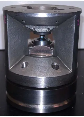
experimental geometries and setups. The experimental technique that will be the focus of

this thesis—nuclear resonant inelastic x-ray scattering (NRIXS)—requires a panoramic

DAC (Figure 2.1). The main feature of a panoramic DAC is that is has large “windows” cut

out of the cylinder, so that detectors can be brought in very close to (~2 cm from) the

compressed sample without compromising the ability to apply a uniform force to the

(38)

(39)

absorbing. However, a cBN seat is preferable over WC on the downstream side of the DAC

if one plans to collect in situ x-ray diffraction (XRD), in order to maximize the range of

accessible diffraction angles. For a similar purpose, our panoramic DACs are also specially

designed with a 90º opening on the downstream side (Figure 2.1; Section 2.2).

To mount a diamond, the diamond and seat are thoroughly cleaned, and a mounting

jig is used to align and secure the diamond roughly in the center of the seat. A mixture of

Stycast 2651 resin and a catalyst in a ratio of 100:7 by weight—prepared immediately

before diamond mounting—is made to serve as the “glue” between the diamond and the

seat. The epoxy should cover the girdle of the diamond and fill in between the girdle and

the seat, but in order to maximize stability of the anvil, the epoxy cannot seep between the

table and the seat (Figure 2.2). When the epoxy is in place, the seat is placed on a heating

plate to allow the epoxy to harden overnight on a low-heat setting.

Once the diamonds have been secured to their seats, they are positioned in the

piston and cylinder sides of the panoramic DAC (e.g., Figure 2.1) using the aligning

screws, which hold the seats flush against the base of the DAC. The cylinder (i.e.,

(a) (b)

Figure 2.2. Diamond mounting and alignment. (a) A black resin is used to mount diamond anvils to a seat; shown here are a WC seat and a diamond with culet diameter of ~100 μm and bevel diameter of 300 μm. (b) Mounted diamonds (of the same dimensions) are aligned in the microscope to bring the culets directly on top of one another; this image provides a close-up view of the resin and anvils.

(40)

downstream in an NRIXS experiment) is equipped with six aligning screws, while the

piston (upstream) only has four. Therefore, common practice is to first secure the diamond

on the cylinder side, and then adjust the aligning screws on the piston side—while looking

through the cylinder-side diamond using a high-magnification microscope—to bring the

culets directly on top of each other. By looking through the microscope while the DAC is

on its side, one can measure the spacing between the culets and perform this alignment

procedure at a variety of spacings, e.g., 500, 200, 100, 30, and 10 μm. Finally, the

alignment of the diamonds is confirmed while they are in contact, and their parallelness is checked by investigating whether any optical fringes are visible. If ≥2 full fringes are

visible, the alignment process can be repeated, or a new orientation of the piston with

respect to the cylinder can be chosen. Since there are three “windows” in the panoramic

DAC, there are three possible orientations that allow for placement of the detectors during

an NRIXS experiment (Figure 2.1); in some DACs, one orientation may produce a better

and more reproducible alignment than the others.

The next step is to prepare a beryllium gasket, which will serve as the walls of the

sample chamber in the DAC. Beryllium (Be) is a hazardous and very soft material, which

makes DAC preparations difficult and limits the pressure range over which the DAC

remains stable. However, the scattered photons in an NRIXS experiment must pass through

the gasket to reach radially positioned detectors (e.g., Figure 2.4), so the more common,

x-ray absorbing gasket materials cannot be used (e.g., stainless steel and rhenium). Early Be

gaskets that were machined for NRIXS experiments were 5 mm in diameter. We use

specially designed Be gaskets that are 3 mm in diameter and machined with a ~400 μm flat

(41)

scattered photons, while the flat area in the center allows for the gasket to rest stably in a

horizontal position on the diamond culets before (and during) indentation.

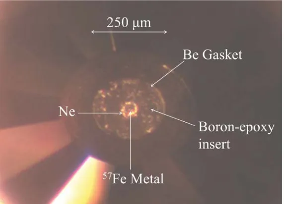
Preparation of a Be gasket for high-pressure NRIXS experiments involves (1)

pre-indenting the gasket, (2) drilling a hole in the center of it, and (3) applying an insert made

of a stiff, low-atomic number material, e.g., boron-epoxy, cBN, or diamond. To pre-indent

the Be gasket, one begins by supporting it on a ring of mounting putty and centering the flat

area over the culets. Indenting the Be gasket to a thickness of ~35 μm work-hardens it prior

to the experiment, resulting in an increased resistance to further deformation during the

experiment and, in turn, improves the chances of achieving higher pressures. A sample

chamber is produced by drilling a hole in the Be gasket using electrical discharge

machining; the drill hole diameter should be ~1/3 of the culet diameter (Dculet) for Dculet≥

250 μm, and equal to or slightly larger than the culet size for Dculet < 250 μm. For larger

culet sizes, a sample chamber large enough for precision sample loading will fit easily into

the center of the culet, leaving some room for sample chamber migration during

compression. For smaller culets, e.g., Dculet= 150 μm, a sample hole that would fit onto the

culet makes sample loading very challenging. Therefore, for small culet sizes, we drill

roughly the entire culet and fill in the hole with the insert material, which reinforces the

shape and size of the sample chamber—thus avoiding rapid thinning of the sample during

compression—as a result of the insert’s high shear strength.

For our high-pressure NRIXS experiments, we use a boron-epoxy insert material

because it is less absorbing at the relevant x-ray energies (~14.4 keV) than cBN and

diamond. To make the boron-epoxy, one mixes amorphous boron and epoxy (in a ratio of

(42)

This procedure should be done under a fume hood and immediately before the first insert is

to be loaded, since the boron-epoxy tends to dry out and become difficult to work with.

Extra boron-epoxy material can be stored under acetone for loading in the days after it is

made. To make the insert, one loads a small piece of the boron-epoxy into the drilled hole

in the Be gasket and compresses it between the diamonds. The insert should fill the entire

hole; spilling over onto the gasket material is fine as long as its distribution is roughly even

and symmetric. Finally, a tungsten loading needle is used to drill a smaller hole in the

boron-epoxy insert, which will serve as the sample chamber. We note that tungsten is used

to avoid 57Fe contamination, which could occur if a stainless steel loading needle is used.

The ideal sample for a high-pressure NRIXS experiment is isotopically enriched in

the resonant isotope (57Fe in our case), and has a starting thickness between 10 to 20 μm.

Both allow for optimal counting rates, while this sample thickness prevents absorption of

the forward scattering signal and significant sample thinning during compression. Ideally,

the sample will be in the center of the culet and not in contact with the gasket or insert

materials, to avoid pressure gradients. When necessary, a few ruby spheres or a piece of

gold will also be loaded as secondary pressure markers, to allow for offline monitoring

while increasing the pressure (e.g., Mao et al., 1986; Dorogokupets and Oganov, 2003;

2006). However, rubies and gold are relatively absorbing materials at ~14.4 keV, and thus

reduce the counting rates of the NRIXS signal. Therefore, we do not load a secondary

pressure marker for our NRIXS experiments on ε-Fe, and instead monitor the pressure in

the sample chamber offline (e.g., while increasing the pressure) using the high-frequency

Raman edge of the diamond from the center of the culet (e.g,. Akahama and Kawamura,

(43)

of ε-Fe and do not depend on the diamond edge calibration.

The final (optional) step is to load a quasi-hydrostatic pressure-transmitting

medium into the sample chamber. For example, pressurized helium and neon gas–loading

facilities are available at GeoSoilEnviroCARS (GSECARS) sector of the APS. If the

experiment does not require quasi-hydrostatic conditions, or the size or geometry of the

sample chamber does not allow for it, then the sample can also be fully embedded in the

boron epoxy insert. To close the DAC and increase the pressure, one uses the tightening

screws. By turning them in sequence two at a time, one applies a parallel force to the

diamonds—and, in turn, the metal gasket—which improves the stability of the sample

chamber with compression.

2.1.2 Our Panoramic DAC Preparations

The analysis presented in this thesis is based on four preparations of modified

panoramic diamond-anvil cells (DACs) with 90º openings on the downstream side (Figure

2.1) and beveled anvils with flat culet diameters of 250 or 150 μm. WC seats were used on

the piston side of the DAC, and cBN seats were used on the cylinder (downstream) side to

maximize the available diffraction angles for our in situ XRD experiments.

For the DACs assembled with 250 μm culets, 80 μm diameter holes were drilled

and filled with boron epoxy. A hole was then drilled in the center of the insert to create the

sample chamber using a loading needle. Into each sample chamber, a piece of 10 μm thick

95% enriched 57Fe foil was loaded, with an area of ~20 × 30 μm. Hydrostatic conditions

were achieved in the sample chamber for our experiments at molar volumes per atom of

57

Fe greater than 5.27 cm3/mol (P ≤ 69 GPa) via the loading of a neon pressure transmitting

(44)

other compression points, the 57Fe foil was fully embedded in the boron epoxy, which

served as the pressure transmitting medium. The pressure in the sample chamber was

monitored offline while increasing the pressure using the diamond-edge calibration

(Akahama and Kawamura, 2006). The final reported pressure was determined from our in

situ XRD andthe Vinet equation of state (EOS) for ε-Fe reported by Dewaele et al. (2006).

For the DACs assembled with 150 μm culet diameters, 125 μm diameter holes were drilled

in the Be gaskets and filled with boron epoxy. A hole was then drilled in the center of the

insert to create the sample chamber, into which a piece of 10 μm thick 95% enriched 57Fe

foil was loaded (~15 × 15 μm in area). Upon compression, the 57Fe foil was fully

embedded in the boron epoxy, which served as the pressure-transmitting medium. Again,

no secondary pressure markers were loaded, and the pressure in the sample chamber was

monitored offline while increasing the pressure using the diamond edge.

(45)

2.2 Synchrotron X-ray Diffraction (XRD)

The theory behind synchrotron x-ray diffraction (XRD) experiments is identical to

that of conventional XRD. Therefore, synchrotron XRD probes the interplanar spacing (d)

of a crystal structure as a function of x-ray energy (λ) and diffraction angle (2θ):

2 sin

nλ= d θ (2.1)

(i.e., Bragg’s Law). In turn, the sample’s unit cell parameters and volume are obtained. The

main advantages of synchrotron XRD are that the flux, high-precision x-ray focusing

hardware, and very sensitive XRD image plates available at synchrotron radiation facilities

allow for the investigation of very small samples, i.e., samples in a DAC.

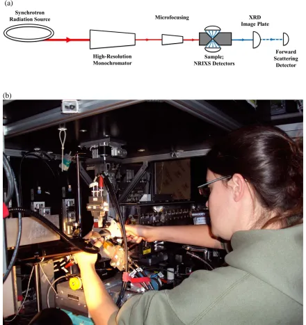
The basic setup for a synchrotron XRD beamline—such as Sector 12.2.2 at the

Advanced Light Source at Lawrence Berkeley Laboratory—is similar to the in-line portion

of the schematic for Sector 3-ID-B at the APS (Figure 2.4). The principal hardware

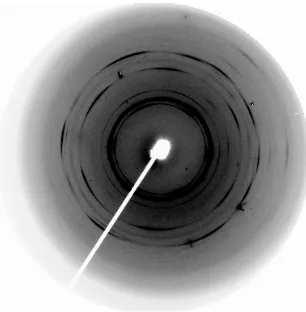
component for synchrotron XRD at both sector 12.2.2 and 3-ID-B is the MAR3450 image

plate, which is a very sensitive detector that allows for high-statistical quality with

low-energy XRD. Sector 12.2.2 is equipped with a Si(111) monochromator, which has an

energy range of 6 to 40 keV, and a sample-detector distance of ~200 mm. For our

experiments in the panoramic DAC, we used E = 30 keV (λ = 0.4133 Å), and determined

the sample-detector distance with high accuracy using a LaB6 standard. Together with our

x-ray transparent cBN seat in the downstream position and angular opening in the DAC of

90º, we have access to a maximum 2θ of ~40º (d≥ 0.6 Å) (Figure 2.5).

Sector 3-ID-B is optimized for NRIXS experiments, but is also equipped for in-line

XRD (Figures 2.4 and 2.5). The MAR3450 image plate is positioned between the sample

(46)

(a)

(b)

(47)

of the x-ray path to allow for in situ XRD before and after an NRIXS experiment. The

incident energy for this in situ XRD is dictated by the NRIXS technique, which requires an

incident x-ray energy equal to that of the nuclear resonant energy of 57Fe (E = 14.4125

keV, λ = 0.86025 Å). The sample-detector distance is ~318 mm, as determined during each

experimental run from the calibration procedure using a CeO2 standard. This suggests a

maximum 2θ of 28.5º (d≥ 1.75 Å), which would corresponds to the maximum pressure at

which the (101) diffraction peak for ε-Fe is accessible of ~100 GPa. However, by

positioning the MAR3450 image plate at a horizontal offset of 35mm from a centered

alignment with the x-ray beam, we were able to increase the maximum accessible 2θ to 33º

(d≥ 1.51 Å). This new 2θcorresponds to a pressure from the (101) diffraction peak of ε-Fe

that is well beyond that of the center of the Earth.

In summary, the majority of the XRD data presented in this thesis are from

synchrotron XRD that was collected in-line at Sector 3-ID-B. The energy of the incident

x-rays was fixed by the NRIXS experiments (E = 14.4125 keV λ = 0.86025 Å), and the

sample-detector distance was calibrated at the beginning of each experimental cycle with a

60-second XRD exposure of a CeO2 standard. Before and after each NRIXS dataset, a lead

plate was inserted directly upstream of the sample stage to reduce detected scattering from

objects in the experimental hutch, while a small hole allowed the incident x-ray beam to

pass through to the sample. A 5 to 10 minute XRD exposure was measured at the sample

position that was probed with NRIXS (Table 2.1). XRD image plate data were analyzed

with the Fit2D software (Hammersley et al., 1996), and the Fityk software (Wojdyr, 2010)

was used to determine the a and c lattice parameters at each compression point by fitting

(48)

(49)

Figure 2.6. Correlation of reported EOS parameter uncertainties. The 1σ error ellipse was calculated as described in Section 2.2, and is centered on the EOS parameters reported by Dewaele et al. (2006). We note that the error ellipse was calculated with V0 fixed to the value given in the caption of Table 2.1.

For our five largest compression points, we observed some texturing in the form of

a loss of intensity in the (002) diffraction peak, likely due to nonhydrostatic conditions at

extreme pressures. To investigate the sensitivity of our results to possible effects from

texturing, we reevaluated the volumes of our five largest compression points with the ratio

c a assigned to be that reported by Dewaele et al. (2006), who measured XRD on ε-Fe to

over 200 GPa with He and Ne as pressure-transmitting media. With the exception of our

measurement at 5.00 ± 0.02 cm3/mol (P = 106 ± 3 GPa), all resulting volumes and

corresponding pressures were within the errors of our original analysis, indicating only a

weak effect from texturing. Finally, XRD spectra were collected for P9 at sector 12.2.2 of

the ALS, approximately 3 months after the corresponding NRIXS measurement at the APS

(Figure 2.5). The energy of the incident x-rays was set to E = 30 keV (λ = 0.4133 Å), and

the sample-detector distance was calibrated at the beginning the experimental run with a

60-second XRD exposure of a LaB6 standard. Observed (100), (002), (101), (102), (110),

and(103) diffraction peaks revealed unit cell parameters a = 2.263 Å and c = 3.598 Å,

which differ slightly from those measured in situ 3 months earlier at Sector 3-ID-B (Table

(50)

(51)

atom of 4.81 cm3/mol and a pressure of 133 GPa, which is consistent with the values

measured at the APS.

2.3 Nuclear Resonant Inelastic X-ray Scattering (NRIXS)

Nuclear resonant inelastic x-ray scattering (NRIXS) is a fairly recent experimental

technique that probes the lattice vibrations (phonons) of select resonant isotopes and, in

turn, their phonon density of states. The timing of the earliest NRIXS experiments

coincided with the 3rd-generation synchrotrons coming online, as a result of their very high

brilliance (∝ flux of a focused beam) compared to earlier synchrotrons. In addition to a

very brilliant x-ray source, NRIXS relies on advanced instrumentation and well-defined

resonances (which are based on the interaction between protons and neutrons in atomic

nuclei) to observe the excitation of nuclear resonant isotopes. One of the most important

features of NRIXS is that it is an isotope-selective technique, which means the signal

originates only from resonant nuclei and, in turn, the measured background is extremely

low. This quality is especially important for experiments at extreme conditions (e.g.,

high-pressure), where counting rates can be restricted by complicated sample environments.

Currently, the NRIXS technique is available at Sector 3 and the High Pressure

Collaboratorive Access Team (HP-CAT, Sector 16) beamlines of the APS; BL11XU and

BL35XU at the Super Photon Ring 8-GeV (SPring-8) in Hyogo, Japan; ID18 and ID22N at

the European Synchrotron Radiation Facility (ESRF) in Grenoble, France; and at P01 at

PETRA–III in Hamburg, Germany. All NRIXS data presented here were collected at

Sector 3-ID-B of the APS.

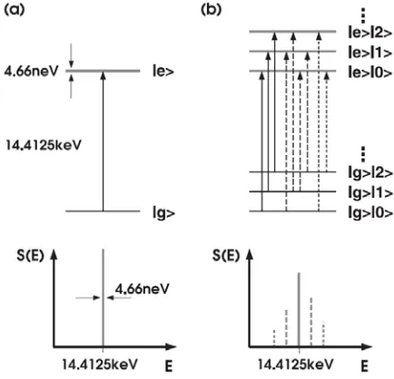
2.3.1 NRIXS Theory

(52)

(53)

excitation probability density (i.e., the number of times resonance is achieved at a given

energy), which is the quantity measured by NRIXS (Sturhahn, 2004). The pair of plots on

the left-hand side show a single transition and elastic peak that correspond to the resonant

excitation of a fixed nucleus, i.e., a nucleus that cannot recoil (ER = 0). Plots on the

right-hand side show similar excitations for 57Fe nuclei bound in a crystal lattice, and one can see

that multiple transitions (and corresponding peaks) are now present.

In the plot presented in the bottom-right corner of Figure 2.7, the most prominent

peak at the center of the spectrum is still the elastic peak (E = 0). This peak represents

recoilless absorption of the lattice during absorption of a photon whose energy equals that

of the nuclear transition energy. In turn, the emitted photon has the same energy, and

resonant excitation of the nuclei can be achieved. This purely elastic (i.e., recoilless)

process occurs over a timescale dictated by the lifetime of the nuclear resonance (which is

inversely proportional to the energy width of 4.66 neV), and ultimately results in the

delayed emission of a photon.

For incident radiation energies on the order of millielectronvolts (meV) larger and

smaller than the nuclear transition energy (i.e., slight “off-resonance”), there are additional

peaks that represent similar resonant nuclear excitations that were achieved by the creation

or annihilation of quantized lattice vibrations (phonons). These peaks are often referred to

as Stokes and anti-Stokes peaks, respectively, because of their conceptual similarity to

those measured with optical spectroscopy techniques. The anti-Stokes peak corresponds to

“phonon-annihilation” because the energy of the incident photon is smaller than the nuclear

transition energy, so the resonance signal must originate from the simultaneous absorption

Thermoelasticity of Hexagonal Close-Packed Iron from the Phonon Density of States

Iron from the Phonon Density of States

Acknowledgements

Abstract

Table of Contents

List of Figures

List of Tables

NOTATION AND NOMENCLATURE

Chapter 1

Introduction

Chapter 2

Experiments