Development of an experimental method to investigate the hydrodynamics in a fluidized bed using PIV and DIA

University of Twente

Faculty of

Science and Technology

Development of an

Experimental Method to

Investigate the

Hydrodynamics in a Fluidized

Bed using PIV and DIA

I. Roghair

Development of an Experimental Method

to Investigate the Hydrodynamics in a

Fluidized Bed using PIV and DIA

Fundamentals of Chemical Reaction Engineering

Faculty of Science and Technology

University of Twente

D-Committee

Chairman:

Prof. dr. ir. J.A.M. Kuipers

Mentor:

Ir. J.A. Laverman

CT-i Mentor: Dr. ir. B.H.L. Betlem

Members:

Dr. ir. M. van Sint Annaland

Dr. ir. G.B. Meier (Basell)

Ir. W. Godlieb

Ivo Roghair

Abstract

An experimental investigation has been performed, studying bubble phase and emul-sion phase behavior in a gas-solid fluidized bed using non-invasive optical techniques. The fluidized bed setup, consisting of two pseudo-2D beds, was operated at various conditions, varying both the bed aspect ratio and the superficial gas velocity. The bed consists of Geldart B glass beads. Experiments were performed by recording images of the bed with a high-speed camera. The images were analyzed by commercial (PIV) and in-house developed software (DIA).

Particle Image Velocimetry has been used to analyze the behavior of the emulsion phase. A method has been implemented to verify that the image recording scheme yielded re-producible time-averaged flow patterns. Also, a vector field stitching program was deliv-ered. In addition, a method is developed to correct for raining particles through bubbles, which severely influence the time-averaged emulsion phase flow pattern. The correction algorithm showed an obvious upward particle flow, whereas the raw PIV results barely yielded any upflow of particles at all. Even after correction, upflow of particles is less pronounced than the downflow. Adaptations of the correction algorithm have been pro-posed to solve this issue.

Corrected time-averaged emulsion phase flow patterns were obtained at 28 different op-erating conditions. It was shown that the upflow of particles is found along the bubble path, from the lower wall region to the top-center region in the bed. The velocity of the particles increased severely with increasing gas flow.

A Digital Image Analysis (DIA) algorithm has been developed, capable of measuring bub-ble properties from an image series. The program was validated and yields accurate and reproducible results.

The DIA program was used to investigate relations for bubble size, velocity and aspect ratio. A theoretical relation, predicting the bubble diameter in a pseudo-2D bed was adapted to include the bed width. The velocity of the bubbles in a pseudo-2D bed can be described asub=KB

√

gdb, in whichKB is a value between 0.6 and 0.7. Moreover, a

Voorwoord

Na zeven jaar studie ligt hier het verslag van mijn afstudeeropdracht. Iets meer dan een jaar geleden begon ik met veel enthousiasme bij de vakgroep FCRE aan een onderzoek naar geflu¨ıdiseerde bedden. Ik heb met veel plezier bij de groep gewerkt, onderzocht gepokerd en geborreld, en ben dus ook van plan dat te blijven doen.

Het afgelopen jaar is er een hoop veranderd. Veel van mijn vrienden zijn afgestudeerd, en zijn verspreid over het land. Mijn vriendin woont nu in het westen, en ikzelf ga nu ook echt op mezelf wonen. Ook ik heb mij moeten beraden op wat ik nou ’later’ wil gaan doen, omdat later naderde. Hier heb ik het met heel veel mensen over gehad, en in de eerste plaats wil ik hen bedanken dat ik met mijn gezeur bij hen terecht kon.

Daarnaast wil ik graag de mensen bedanken die mij hebben geholpen om iets moois van mijn afstuderen te maken. Van Christiaan heb ik veel nuttige tips gekregen over het reilen en zeilen met de PIV opstelling. Willem stond altijd klaar als ik extra re-sources op het computercluster nodig had en de kennis van Wouter met betrekking tot programmeren heb ik ook goed kunnen gebruiken. Wim heeft superwerk gedaan door de camerastandaard te maken, en tevens omdat hij de door mij gesloopte kolom weer heeft gerepareerd. Bij Niels kon ik ook altijd aankloppen, die het elke keer voor elkaar kreeg om mijn vragen heel helder uit te leggen. Martin wil ik bedanken omdat hij mij na mijn stage heeft gewezen op de mogelijkheden van afstuderen bij FAP. Ook Hans ben ik erkentelijk dat ik de opdracht hier kon uitvoeren. Tevens wil ik alle commissieleden bedanken voor hun idee¨en en de discussies die we hebben gevoerd.

Jan Albert wil ik heel erg bedanken voor de gezelligheid, advies en begeleiding gedurende het project. Naast het feit dat je prima gezelschap op borrels bent, heb je me ook enorm geholpen door zoveel teksten van mij te corrigeren. En vele zelfs meerdere malen, waarin je de zaken die ik niet had verbeterd stug nog een keer aanstreepte.

Met dit verslag en de komende presentatie rond ik als het goed is ook mijn studie Chemische Technologie af. Het leven in Enschede was een geweldige tijd, en dat is te danken aan een groot aantal mensen.

Beste vrienden, door jullie zijn de afgelopen zeven jaar onvergetelijk! Vakanties, borrels, studiereis, feesten en wijnproefavonden. Jullie zijn toppers, bedankt!! Martin en Bas wil ik hier trouwens nog even uitlichten. Jullie zijn een stelletje toffe knullen, en ik zal onze idiote gesprekken en het –zo mogelijk– nog vreemder aangeklede huis erg missen. Er is ´e´en iemand die mij met haar lach weer uit een dip kan halen, die me verteld wanneer ik moet stoppen met werken, waarmee ik al mijn geluksmomentjes deel en waarbij ik mijn hart kan uitstorten. Lieve Suzanne, dank je wel voor al deze geweldige momenten!

Bovenal mag ik me gelukkig prijzen met mijn ouders. Naast natuurlijk de financi¨ele steun gedurende mijn studie, waar ik erg dankbaar voor ben, ben ik ook heel blij met de vaste thuisbasis in Zoetermeer waar ik altijd kan aankloppen. Bedankt voor jullie support de afgelopen jaren, voor de adviezen en gesprekken die we hebben gehad, en voor de motivatie die ik soms nodig had. Jullie zijn wereldouders!

Contents

1 Introduction 1

1.1 Gas-Solid Fluidization. . . 1

1.2 Project Scope . . . 2

1.3 Project Goals . . . 3

2 Theory 5 2.1 Introduction . . . 5

2.2 Emulsion phase behavior . . . 5

2.3 Bubble behavior . . . 9

2.4 Pseudo-2D to 3D . . . 14

3 Application Development 17 3.1 Introduction . . . 17

3.2 Digital Image Analysis. . . 17

3.3 PIV Raining Particles Correction . . . 20

3.4 Stitch program . . . 23

3.5 Verification of Image Acquisition scheme . . . 24

3.6 Data Flow Diagram . . . 25

4 Experiments 29 4.1 Introduction . . . 29

4.2 Experimental setup . . . 29

4.3 Summary of operating conditions . . . 32

5 Results and Discussion 34 5.1 Hydrodynamics. . . 34

5.2 Bubble properties measurements . . . 39

5.3 Two-way coupling . . . 45

6 Conclusions and Recommendations 48 6.1 Conclusions. . . 48

6.2 Recommendations . . . 49

References 51

A PIV Design Rules 54

B Edge Detection 56

C Particle flow patterns 58

Symbols and Abbreviations

Symbols

A0 Catchment area m2

Ab Aspect ratio of a bubble —

Abed Cross sectional area of the bed m2

AF Acceleration factor —

Ar Archimedes number —

c Proportionality constant (∼2) —

d32 Sauter mean diameter m

db Bubble diameter m

db,0 Initial bubble diameter m

db,max Maximum bubble diameter m

dp Particle diameter m

dbed Bed diameter / width m

dx, dy Horizontal, vertical span of a bubble m

dv, ds Volume, surface diameter m

fb Bubble frequency s-1

ft Fraction of tracer particles (≡1) —

FI In-plane particle loss correction factor —

FO Out-of-plane particle loss correction factor —

FT Parameter for particle shape —

F∆ Velocity gradient in interrogation area —

g Gravitational constant m·s-2

h, hbed Fixed (unfluidized) bed height m

i Position on digital image px

I Intensity matrix —

I0, I00 First, second image —

hIi Overall/Average image intensity —

j Position on digital image px

k Position on digital image px

KB Bubble rise velocity constant —

` Emulsion phase velocity vector (identical tou m·s-1

M Conversion factor px−→mm mm·px-1

n Number of bubbles, number of classes —

N Interrogation zone size px

N1, N2 Position of bubble nose —

Nf Number of vector fields —

NI Number of particles in interrogation area —

Nx, Ny Total number of pixels in horizontal, vertical direction px

P Perimeter m

Symbols(continued)

ra Range for local average px

rb,2D/3D 2D, 3D radius of bubble m

ˆ

R Correlation peak —

RD Displacement peak —

Sb Surface of bubble in a pseudo-2D bed m2

SF Collin’s Size Factor —

t Pseudo-2D bed thickness m

T Threshold intensity —

u0 Superficial gas velocity m·s-1

ub Bubble rise velocity m·s-1

ug,p Gas velocity through the particle phase m·s-1 umb Minimum bubble superficial gas velocity m·s-1

umf Minimum fluidization gas velocity m·s-1

up Predicted particle velocity m·s-1

uz Vertical particle phase velocity m·s-1

u Bubble velocity vector m·s-1

x, z Lateral, Axial position px, mm

xc, yc Average horizontal, vertical displacement px

z Vertical position above distributor m

Greek Symbols

ε∗ Binary porosity matrix —

εm Porosity of a fixed bed —

εmf Porosity at minimum fluidization gas velocity —

ε2D,3D Porosity in a pseudo-2D / 3D bed —

φs Sphericity factor —

φv,b Volumetric bubble flow, Visible bubble flow m3·s-1

λ Bulk viscosity kg·m-1·s-1

µg Gas viscosity kg·m-1·s-1

ψ Ratio between observed bubble flow and excess gas flow —

ρg Density of gas kg·m-3

ρp Density of particle kg·m-3

σ Standard deviation —

ϑ Wall influence parameter —

θd Angle between leading and trailing bubble ◦

Abbreviations

DBM Discrete Bubble Model

CARPT Computer Aided Radioactive Particle Tracking DIA Digital Image Analysis

DPM Discrete Particle Model CRiB Counter Raining in Bubbles FBR Fluidized Bed Reactor GB Glass Beads

MFC Mass Flow Controllers PE Polyethylene

PEPT Positron Emission Particle Tracking PIV Particle Image Velocimetry

RMS Root Mean Square SMD Sauter Mean Diameter TFM Two-Fluid Model

Chapter 1

Introduction

In this chapter, first the basic principles of fluidization will be discussed. Then, the use of fluidization in industry is outlined, followed by the scope of the project. The last section of this chapter defines the goals of this project.

1.1

Gas-Solid Fluidization

Fluidization is a phenomenon transforming a fixed bed of particles, which has static behavior, to a dynamic state. This is done with an upward fluid flow through the bed. In industry, fluidization is performed in Fluidized Bed Reactors (FBR). These are used in a wide field, e.g. for the polymerization of olefins, drying of starch and combustion of coal, but even the cinema popcorn machine uses the principle of fluidization[1;2]. A particle system in fluidized behaves like a liquid. For example, the surface remains hor-izontally when the bed is tilted, and objects with a higher density than that of the bed sink into the bed.

Fluidized bed reactors show an excellent mass and heat transfer due to rapid mixing of the particles. Therefore, it is often used in large scale operations. Moreover, it responds slowly to changes in temperature and provides an excellent gas-solid contact.

Its disadvantages are nonuniform particle residence time, erosion of the vessel and in-ternals due to the solid phase and a low gas conversion rate[3]_.

In this thesis, gas-solid fluidization is considered. Gas is distributed over the column in which the particle bed is present. Although depending on the process, this is normally done by a bottom plate with gas inlets distributed over the surface of the distributor. The particles experience a drag force induced by the gas flow. At low gas flow rates, the gas flows through the interstitial volume between the particles (packed bed state, figure1.1a). Increasing the superficial gas velocity makes the particles to move further apart; the bed expands as the voidage between the particles grows larger. Bed expan-sion continues until the gas flow rate reaches a certain value. When the gravitational force equals the drag force of the gas on the particles, particles start to float (figure 1.1b). This gas flow rate is called the minimum fluidization gas velocity,umf.

At gas flow rates above umf, bubbles start to form above the distributor as shown in figure 1.1c. The bubbles rise through the particle phase due to the buoyancy force. Bubbles grow larger while rising due to gas entrainment and coalescence. Depending on the particle classification, bubbles may also break-up. The existence of bubbles in a fluidized bed causes mixing of the particles. The bubbles induce a stirring action and convective particle transport through the bed. More on this topic will be discussed in chapter2.

1.2. PROJECT SCOPE

(a) (b) (c) (d) (e)

Figure 1.1: (a)Fixed bed state(b)Expanded bed at minimum fluidization gas velocity (c) Bub-bling fluidized bed(d)Slugging regime(e)Entrainment of particles[3]

the bubbles to be restricted by the walls, another regime is reached, called slugging (figure 1.1d). The wide bubbles reach almost from wall to wall, while particles mainly rain down the wide bubbles. Entrainment of particles by the gas flow is shown in figure 1.1e. This work investigates the bubbling fluidization regime.

1.2

Project Scope

Gas-solid fluidized beds are widely employed in the (petro) chemical industry. This research is performed in the scope of polymerization reactor systems. Together with the liquid slurry process and the solution process, the fluidized bed process is com-monly used. An example of a gas phase olefin polymerization process is the so-called UNIPOLTM _{process, depicted in figure 1.1. The gas phase polymerization process}

pro-duces polyethylene (PE) with large ranges of both product densities and molecular weight distribution[4]_{. Monomer gas is fed trough the bottom of the column,}

fluidiz-ing the polymer particles and actfluidiz-ing as a reagent. Heat removal is an important issue for this process, because the polymerization reaction is highly exothermic and the tem-perature should not exceed the melting point of PE. The produced heat is transported through the reactor by solids mixing (convective heat transport), and can be removed by emerging gas and cooling at the walls. Alternatively, it is possible to remove heat by operating FBR in condensed mode, i.e. the monomer is partly added to the reactor as a liquid, which is evaporated by the heat of the polymerization reaction. Despite this solution, heat transfer through the solids phase is a key factor to further improve heat removal. Insight in the macroscopic circulation patterns will be beneficious for a higher efficiency heat removal, and therefore the production can be optimized.

enor-Freeboard area

Unreacted gas to recycle

Catalyst F_cat

Product Q

Monomer gas inlet u₀

Figure 1.2:UNIPOLTM_process[4]

mous progression in computing power, models of a full-scale reactor predicting the flow in the smallest detail are still outside limits. However, closure relations of the detailed flow structures can be obtained by small-scale simulations, and provided to large-scale models.

Different approaches of modelling the two-phase flow are therefore performed. At the highest detail level, lattice-Boltzmann simulations are performed to provide closure re-lations for the drag force of the gas on the particles[5]_{. Small systems can be simulated}

in the Discrete Particle Model (DPM), which is used to model the trajectories of indi-vidual particles by Newton’s second law of motion (e.g. Van Der Hoefet al.[6]_{). Particles}

are the discrete entities, through which the gaseous phase flow is solved using the volume-averaged Navier-Stokes equations. A larger scale approach involves modelling of the particle phase as a continuum. A Two-Fluid Model was designed by Kuipers et al.[7]_{, considering the particle phase and the gaseous phase as interpenetrating}

Newto-nian fluids. A Discrete Bubble Model (DBM) of a bubble column was adapted to model fluidized bed hydrodynamics[4;8]_{. In this model, the bubbles are modelled as the}

dis-crete entities which can collide and coalesce. The particle phase flow is solved using the Navier-Stokes equations.

In order to validate the models, experiments must be performed to verify the hydrody-namics predicted by the models with experimental data. The qualitative flow pattern of the particle phase is already known, but quantitative information on particle phase flow is still scarce. The interaction between the two phases has also not been quantified yet. Raising the question, what influence bubble movement has on the particle phase.

1.3

Project Goals

1.3. PROJECT GOALS

The flow patterns can be used to obtain the particle flow through the bed in axial and lateral directions.

Bubble behavior and the influence of the bubbles on the particle phase is investigated using a newly developed computer program. This program detects bubbles and extracts bubble properties from images of a pseudo-2D fluidized bed. Bubble properties of pri-mary interest are position, size and velocity.

Chapter 2

Theory

2.1

Introduction

This project focuses on obtaining fundamental information on the hydrodynamics of the emulsion phase, the behavior of the bubble phase and bubble-emulsion phase in-teraction in a bubbling gas-solid fluidized bed. Literature available on these subjects will be discussed here.

Two parts can be distinguished in this chapter. The first part discusses parameters which influence the emulsion phase behavior, followed by an outline of the experimen-tal method (PIV) used to measure the hydrodynamics of the emulsion phase. The second part concerns correlations predicting the behavior of the bubble phase. Consequently, a method to experimentally acquire bubble phase behavior non-invasively (DIA) is dis-cussed. At the end of this chapter a short outline on 2D - 3D conversion is given.

2.2

Emulsion phase behavior

2.2.1

Hydrodynamics

The particulate phase in a bubbling fluidized bed can be considered as a flowing contin-uum. The flow is induced by bubble movement. In the wake behind a bubble, particles are dragged upward along the bubble path as shown in figure 2.1a. Particles stream down along the sides of the bubble. Because bubbles mainly form at the lower wall region and have the tendency to move towards the center of the bed as they rise, the main upward flow of particles is expected between the core and the wall region.

Various flow patterns have been defined for different bed aspect ratios and superficial gas velocities. For example, it is stated[3] _{that at low gas flow rates and shallow beds,}

particles flow upward along the wall and down through the center of the bed. This pattern is reversed at higher gas flow rates and aspect ratios which approach unity. Moreover, in deep beds a second vortex ring emerges which, especially at high gas flow rates, dominates the overall particle circulation pattern[1;3;9]_{. This pattern can be found}

in figure2.1b.

Particle classification

In 1973, Geldart[10] _{proposed a method to classify particles based on their size}

2.2. EMULSION PHASE BEHAVIOR

Solids Gas

(a) (b)

Figure 2.1: (a)The path of the bubbles starting at the walls and moving towards the center of the bed, hereby taking the particles upward along their path. The emulsion phase downflow can be found in the center and at the walls of the bed.(b) The general particle flow pattern in deep beds. From Kunii and Levenspiel (1991)[3]

Channeling of gas is likely to occur in these particle systems. Class A consists of small and/or low density particles. They are easily fluidized. Geldart B particles are sand-like, and are also easy to fluidize. The main difference between class A and B particle types is that bubbles in Geldart A particle systems are restricted in their size due to break-up. The largest particles are grouped as Geldart D particles, which are difficult to fluidize, particularly in deep beds[3;10].

Besides, the gas flow through bubbles is different in these particle systems. In Geldart A and B particles, gas flow through the bubbles circulates and forms a cloud around the bubbles. In Geldart D systems, the gas mainly goes through the bubbles, and flows upward.

The scope of this project comprises olefin polymerization reactors, in which the particle size depends on the residence time of a catalytic particle in the reactor. Particles in these types of reactors range typically from 0.25 to 1.0 mm[1]_{. The polyolefin particles}

are therefore mainly found in the Geldart B region.

The minimum fluidization gas velocity depends strongly on the chosen particles. To cal-culate the minimum fluidization velocityumf, the following relation is proposed in Kunii

and Levenspiel (1991)[3;11]_:

umf =

µg ρgdp

p

(27.2)2_{+ 0.0408Ar−27.2 (2.1)}

where the Archimedes numberAr is defined as:

Ar=d

3

pρg(ρp−ρg)g µ2

g

(2.2)

In this project, umf is determined experimentally in a pseudo-2D bed by a pressure

10 50 100 500 1000

Figure 2.2:The Geldart classification of particles for air at ambient conditions (from Kunii and Levenspiel (1991)[3]_.

Particle Tracking

The measurement of emulsion phase flow in a fluidized bed can be performed with par-ticle tracking techniques. These techniques are non-intrusive, and can be performed in relatively large 3D beds. Positron Emission Particle Tracking (PEPT) and Radioactive Particle Tracking (RPT) methods are most often used in this respect. In RPT, a γ-ray emitting particle is followed through the emulsion phase in three direction by γ-ray detectors. PEPT uses particles which emit positrons due to β-decay. When a positron and an electron meet, they annihilate and convert their masses into energy, which is released by electromagnetic radiation. Twoγ-rays are emitted almost exactly back-to-back. The trajectory is called the annihilation vector. If two γ-rays are detected within the resolving time window, this vector is determined. The particle is positioned at the intersection of several vectors.

Apart from its radioactive properties, a tracer particle is identical to the other parti-cles in the bed. By recording the trajectory of the particle, time averaged results can be obtained, as well as the fluctuations in particle position in relatively large setups. However, instantaneous total flow behavior cannot be studied, as only a single particle is labelled[12]_{. Steinet al.}[13] _{performed PEPT experiments in cylindrical beds with}

Gel-dart B particles. They found ascending particles in the core region, downflow at the wall region and particles in the bubble trajectory, move both up and downward. They also mention that the average emulsion phase upward velocity is about half of the bubble velocity, independent of the superficial gas velocity. This conclusion however, is based on the calculated bubble velocity and diameter, using theoretical equations.

This result was confirmed by Mostoufi and Chaouki[14]. They performed RPT experi-ments in order to investigate particle flow structures in a fluidized bed, and they too found ascending particle clusters in the center of the bed, whereas descending clusters were mostly found in the wall region. The authors also related emulsion phase motion to the velocity of a rising bubble. It was noted that particles in the wake of the bubble ascend proportional to the velocity of the bubble. The bubble velocity however, was not measured directly, but rather obtained from theoretical relations.

2.2. EMULSION PHASE BEHAVIOR

2.2.2

Particle Image Velocimetry

Particle Image Velocimetry (PIV) is an experimental method to obtain instantaneous macroscopic flow patterns of a system. PIV is a non-intrusive, optical technique, orig-inally developed to study flows in liquid or liquid-gas systems. These systems usually work with tracer particles that are injected in the flow of interest. In this case, PIV is performed to study the flow of the emulsion phase, first performed by Bokkers[4] _and

later by Link[15]_{. In the case of PIV on granular media, tracer particles are not always}

needed as the particles themselves are being tracked[16–18]. A drawback of using an opaque system such as a fluidized bed, is that visual access can only be obtained at the wall. Hence, a pseudo-2D bed is required to measure the macroscale circulation patterns in the fluidized bed.

The emerging instantaneous patterns can be used to obtain the time-averaged particle circulation pattern through the whole bed. In addition, instantaneous flow fields can be used to gain detailed insight in other complex phenomena, such as the flow around ris-ing bubbles. In this project, PIV calculations are performed usris-ing DaVis software from LaVision. This section covers the basics of PIV. AppendixAdiscusses design rules that have to be taken into account, which are specified in literature.

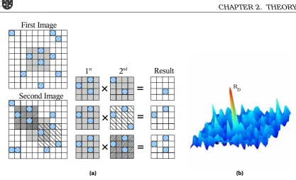
The basic principle of PIV consists of spatial cross-correlation of two consecutive im-ages. Thereby an instantaneous flow pattern is obtained of the entire photographed area. To obtain good resolution, the images are divided in so-termed interrogation zones. For each interrogation zone, individual correlation between the two images is performed. An example is given in figure2.3a, where a pattern on the first image (solid area) is compared to three equal sized areas on the second image (the solid, dashed and fine-dashed areas). This results in spatial cross-correlation peaks (figure2.3b) for every interrogation zone. The highest value indicates the most likely displacement of that par-ticular interrogation zone. There are several parameters that influence the displacement peakRD(x, y):

RD(x, y) =NI·FI(x, y)·FO·FT(x, y)·F∆(x, y) (2.3)

PIV only determines the movement in a 2D plane. Therefore, particles moving out of the plane (i.e. perpendicular to the field of view, FO) and particles moving out of the interrogated area parallel to the field of view (FI(x, y)) account for a loss of correlation. The error caused by these parameters can be minimized by decreasing the delay be-tween the two images. The shape of the peak is influenced by the shape of the particles (FT(x, y)) and the velocity distribution in the interrogation zone (F∆(x, y)). The spatial

cross-correlation of the images is calculated with equation2.4.

ˆ

R[x, y] = 1

NxNy Nx

X

i=1 Ny

X

j=1

(I0[i, j]− hIi) (I00[i+x, j+y]− hIi) (2.4)

Note that the overall image intensity hIiis subtracted from both images before cross-correlation takes place. This reduces the background cross-correlation.

First Image

Second Image

1

2

Result

(a)

R_D

(b)

Figure 2.3: (a) correlation of two images using a 4x4 interrogation area. Three correlation in-stances are shown, of which the bottom window shift shows the most likely particle relocation.(b)spatial cross-correlation plot. The most likely displacement is given by the high peak, called the dislocation peakRD.

2.3

Bubble behavior

2.3.1

Gas phase transport

When the superficial velocity is raised above the minimum bubble superficial gas ve-locity umb, bubbles start to form just above the distributor. In the case of Geldart B

particles, umb is found at a superficial gas velocity u0 slightly exceeding the minimum

fluidization velocity. At these conditions, bubbles start to form, causing circulation pat-terns of the solids[3]. On average, bubbles move as depicted in figure 2.1a, from the lower wall regions towards the center of the bed as they rise.

The two-phase theory of fluidization states that the excess gas flow, i.e. (u0−umf), is

visible as rising bubbles. The observed bubble flow ratio to the two-phase expected bubble flow can be expressed as:

ψ=

observed bubble flow excess flow from 2 phase theory

= φv,b (u0−umf)Abed

(2.5)

However, numerous experiments have shown that the observed bubble flow is less than the excess flow. Hence, the transport of gas through the bed must be described by addi-tional means besides bubbles. Geldart[19]_{proposes three mechanisms by which the gas}

moves through the bed; interstitial gas flow through the particle phase, gas flow by the rising bubbles and superimposed gas flow through bubbles. Geraet al.[20] _have

inves-tigated the through flow of gas between two interacting bubbles. They also found that the path between two bubbles taken by the gas has a lower porosity than elsewhere in the bed, which is attributed to the superimposed gas flow. For Geldart B particles and

2.3. BUBBLE BEHAVIOR

2.3.2

Bubble properties

Several relations have been proposed to describe bubble properties in a fluidized bed. Besides its size, the velocity of a bubble can be predicted, as well as parameters which define the shape of a bubble.

Bubble size

Bubbles grow due to gas entrainment and coalescence. Bubbles shrink due to gas leak-age and break up. Bubble size and growth depend strongly on the particle type that is used. Using very small particles restricts the maximum size of the bubbles rigorously (the roof collapses in small particle systems), whereas bubbles in Geldart B and D par-ticle systems seem to grow without limits[3]_.

The bubble diameter is commonly expressed as the equivalent diameter of a spherical bubble (for 3D beds) or a circular shape (in pseudo-2D systems). A number of correla-tions are found in literature to describe the bubble diameterdbin a fluidized bed[3;11;21].

The Darton relation gives the bubble diameter as a function of the height above the distributor plate:

in which4√A0 = 0.03m for a porous plate. This correlation is derived for 3D fluidized

beds and Geldart B particle types. Mori and Wen describe bubble growth as[3;11]_:

db=db,max−(db,max−db,0)·e

−0.3z

dbed _(2.7a)

in which the maximum bubble diameterdb,maxcan be calculated with eq.2.7b:

db,max= 0.65hπ

and the initial bubble diameterdb,0 above a porous plate distributor is expressed as:

db,0= 0.376 (u0−umf)2 (2.7c)

Alternatively, the Hilligardt-Werther correlation is described as followed:

db=db,0(1 + 27 (u0−umf))

using an initial bubble size of:

db,0=

Hilligardt-Werther (2.8) equations are valid for a 3D bubbling fluidized bed. Alterna-tively, one could use the relation of Shenet al.[23]_{. This relation is valid for a}

pseudo-2D fluidized bed, and was obtained from DIA experiments. Note that the equation is analogue to the Darton relation with a higher coefficient and different powers. Their experimental data and the proposed relation is given in figure2.4a. The correlation is given as:

db= 0.89 [(u0−umf)(z+ 3.0A0/t)]2/3g−1/3 (2.10)

(a)

Figure 2.4: (a)The relation of Shenet al.[23]fitted to experimental data(b)The radial distribution of bubble-gas flow. From Werther (2002)[1]_.

Bubble Rise Velocity

As bubbles grow, they rise faster through the bed. Depending on the bubble diameter, the terminal velocity of a single unhindered spherical-cap gas bubble can be expressed with the Davies and Taylor expression[3]:

ub=KBpgdb (2.11)

In 3D beds, the value of the bubble rise velocity constantKB is commonly set to0.711. The value forKB is still under debate for 2D cases. It is reported thatKB ≈0.50or even

0.41for 2D bubbles[24;25]_{. However, also higher constants are obtained, e.g. by Shenet} al. who derived a value of0.8 - 1.0[23]. It is found that equation 2.11describes bubble velocities within a 30% range. The large range is due to breakup and coalescence which alters the bubble diameter significantly[25]_.

The velocity of a swarm of bubbles can be described with an extended form of the Davies–Taylor expression (eq.2.11):

ub= (u0−umf) +KB

p

gdb (2.12)

In order to account for wall effects, Werther[1]_{proposed a relation that includes the bed}

diameter:

Another way to incorporate wall influences on the bubble rise velocity is to include a size-factor (SF) in the Davies–Taylor relation (2.11), as proposed by Collins (1967)[26]_:

ub=KB

p

gdb(SF) (2.14a)

which represents the rise velocity of a single, isolated bubble[27]_{. The size factor}

2.3. BUBBLE BEHAVIOR

The velocity of a bubble is also dependent on the presence of other bubbles. Krishna and Van Baten (2001) proposed a relation to include bubble acceleration imposed on a bubble by using the Davies-Taylor-Collins equation (2.14a) as a basis.

ub=u0b(AF) =KB

p

gdb(SF)(AF) (2.15a)

In this equationAF is the acceleration factor expressed as:

AF = 1.64 + 2.7722(u0−ug,p) (2.15b)

Here, ug,p equals the gas velocity through the particle phase interstitially. It is worth mentioning that the interstitial gas flow apparently does not depend on the size of the bubbles and distance between the bubbles. However, one would expect it based on the superimposed gas flow as discussed by Geraet al.[20]_.

Bubble shape

In A and B types of particles, the shape of a bubble is usually a spherical cap (at atmo-spheric pressure)[9]_{. Interaction between bubbles is known to change the properties of}

a bubble. Besides common bubble parameters such as velocity, direction and size, the shape of a bubble is also distorted as a result of its presence close to another bubble. A tailing bubble accelerates under influence of a leading bubble in the direction of the leader. In this process, the leading bubble is flattened whereas the tailing bubble is elongated in the direction of the leader as a result of increased gas flow in that direc-tion.

The shape of a bubble can be characterized with two different parameters. The first one is the aspect ratioAb, that can be described by the horizontal and vertical spandx

anddy, as shown in figure2.5:

Ab=dy

dx

(2.16)

The second shape characteristic parameter is the sphericity factor S. The sphericity is obtained by dividing the circumference of a circle with equivalent diameter db by the detected circumference (perimeter)P of a bubble.:

S =πdb

P (2.17)

d_y

d_x

0 0.6 0.9 1

Figure 2.6: (a)Sphericity distribution results of Limet al.[28]_{(b)Aspect ratio distribution results}

of Limet al.[28]

The distribution of these parameters was investigated by Lim et al.[28] _{and Caicedo et} al[29]_{. Results of Limet al. are given in figure 2.6. This figure shows that the majority}

of the bubbles have an aspect ratio of 1, whereas the mean sphericity is found to be about 0.9. These parameters were measured at 10 cm above the distributor plate at a superficial gas velocity of 4umf. Caicedo et al. however, find lower sphericity values of about 0.7 and aspect ratios mainly above 1. The difference with the work of Limet al. is the superficial velocity, which Caicedo et al. set to l.4umf. Apparently, a lower superficial gas velocity gives rise to vertically stretched bubbles. However, this would not be expected as bubble-bubble interaction is more likely to occur in systems with higher superficial gas velocity. Various bubble properties have been discussed in this section. These properties can be investigated by digital image analysis; an algorithm capable of analyzing a series of images in order to extract the information needed. Main issues on digital image analysis algorithms described in literature are outlined in the following section.

2.3.3

Digital Image Analysis

Digital image analysis (DIA) is performed to investigate bubble parameters such as the position, velocity and size from a series of digital images in a freely bubbling pseudo-2D fluidized bed. The obtained data are used to determine relations describing the bubble behavior by statistical analysis.

A DIA program generally obtains an image and preprocesses it. Consequently, it seg-mentates the two phases (emulsion and bubble phase) by comparing the gray level of every pixel with a threshold value. In a postprocessing step, bubble properties are de-termined.

The advantage of DIA is that it is capable of measuring at a high resolution, has a po-tential high degree of automation and the flow pattern is not disturbed by probes or sensors. However, similar to PIV, visual access to the bed is required. Therefore, images are taken from a pseudo-2D fluidized bed.

Pioneers in the field of DIA on fluidized beds are Lim and Agarwalet al.[28;30;31]_{. But also}

other groups[23;25]_{have described their algorithm in literature. This section outlines}

subse-2.4. PSEUDO-2D TO 3D

quent frames. The development of the DIA software used in this research is described in section3.2.

Phase segmentation step

Lim and Agarwal et al. place the light source behind a pseudo-2D bed. The bubbles they record are therefore seen as light objects, whereas the opaque particle phase is not illuminated. They used a threshold for the segmentation process, which was defined as the minimum between the peaks of a bimodal gray value histogram. For their algorithm, images should have high contrast between the phases and homogeneous lighting. Shen

et al.[23]_{determined a constant threshold by analysis of a whole image series. Muddeet} al.[25]_{used an adaptive threshold value, determined by analysis of the variation of gray}

values in the image. They preprocessed the images before segmentation is performed.

DIA postprocessing

The position of a bubble is usually set to the center of gravity and the size (projected area of the bubble) is equivalent to the adjacent bubble pixels. The position of a bubble on subsequent frames is used to measure the velocity. The bubble velocity measure-ment is based on the shift of the center of gravity between two consequent frames. The displacement of a bubble must be within a predescribed range. If multiple bubbles fulfill this criteria, the smallest positive displacement is used for the velocity measure-ment[25]_{. In most cases in literature, a video camera was used, which had a fixed frame}

rate of 25 fps (frames per second) with a fixed delay between the images of 40 ms or 20 ms. Between 2000[28] _{and 10000}[23]_{images were used for statistical analysis.}

Other parameters, such as the gas hold-up, the aspect ratio and the shape factor were also detected in the algortihms discussed[23;25;30]_{. As mentioned in section 2.3.2, the}

distribution of the shape factor and aspect ratio was measured[28;29]_{. However, the}

ve-locity dependence of the aspect ratio is not yet investigated, although it is proposed that the aspect ratio might be of significant influence on the bubble velocity[30]_{. It was also}

found that bubbles smaller than the depth of the pseudo-2D bed are not fully visible because they do not stretch from the front to the back wall, as pointed out by Limet al.[28]_{. Therefore, bubbles that are smaller than the bed depth, are not taken into}

ac-count.

DIA and PIV are used with images that are obtained from a pseudo-2D fluidized bed. In order to interpretate results for three dimensional reactor systems, the wall effects in a pseudo-2D systems are outlined in the following section.

2.4

Pseudo-2D to 3D

The geometry of a pseudo-2D fluidized bed restricts the multiphase flow in one dimen-sion, which influences the flow behavior. For example, bubbles in a pseudo-2D bed rise slower as compared to identical frontal diameter bubbles in a 3D bed[10;25]_{. Also, the}

observedumf is usually larger for a 2D bed as compared to a 3D bed. In this section,

first the effect on the particle phase will be discussed. Then a number of methods are given to convert bubble properties between the two geometries.

Particle phase

Compared to a cylindrical (3D) reactor, a pseudo-2D fluidized bed has a large internal surface area to volume ratio. Using a two-fluid model, Kobayashiet al.[32] _{showed that}

bed. Villa-Briongos et al.[33] _{provide a scaling method that is based on deterministic}

chaos theory. They define a geometry independent Kolmogorov entropy based on fluc-tuations at the bed surface, under the assumption that these flucfluc-tuations provide a measure for the hydrodynamics throughout the entire bed. It was found that for Gel-dart B and D type particles, the hydrodynamics of 2D and 3D systems are qualitatively comparable.

Concerning the porosity of the particle phase, Link assumes a relation to calculate the porosity in a 3D fluidized bed with data obtained from a pseudo-2D bed by:

ε3D= (ε2D) 3

2 _(2.18)

This relation is obtained analytically by assuming that the particle configuration in a 3D bed is equivalent to the particle configuration at the front plate of a 2D bed.

Bubble phase

Predicting the diameter of a bubble in a 3D bed with experimental pseudo-2D data is modelled in several ways. First of all, the Sauter Mean Diameter (SMD) of a pseudo-2D bubble could be used to transform the volume/surface ratio to a spherical bubble. The SMD is defined as:

SMD=d32=

in which i is the number of bubbles, ds is the surface diameter and dv is the volume diameter. In the case of bubbles in a pseudo-2D bed, it is argued that bubbles are of cylindrical shape, with the ’top’ and ’bottom’ of the cylinder found at the frontal and back plate. The surface area which is able to expand is the curved surface of this cylinder. The surface diameter ds can therefore be set to the area allowed to expand

through the bed:

in which t equals the depth of the column, anddb the diameter of the 2D bubble. The volume diameterdv can now be described as:

dv=

Geldart (1970)[19] _{has found that due to out-of-line coalescence, bubbles in a 3D bed}

typically grow larger than in a 2D bed under comparable conditions. The diameter can be calculated for an idealized case, without accounting for side-wall effects and out-of-line coalescence, with the data obtained from a pseudo-2D fluidized bed using images and probes simultaneously. The bubble concentration in a 2D bed and the point bubble frequency obtained from the probes describe a relation for the bubble concentration in a 3D bed:

2.4. PSEUDO-2D TO 3D

Chapter 3

Application Development

3.1

Introduction

Several programs have been developed to analyze, validate and post-process the experi-mental results. The programs are written in the C programming language. This chapter will discuss the development of these program and describe the way they programs work.

First, the development of the Digital Image Analysis (DIA) program is described in sec-tion 3.2. DIA is used to analyze digital images of the bed, separate the bubbles from the emulsion phase and determine bubble properties such as size, location and veloc-ity. A post-processing method to correct PIV measurements is proposed in section3.3. In section 3.4 the Stitch program is discussed. This program combines multiple time-averaged PIV vector plots for cases in which the bed could not be recorded as a whole. In section3.5, a program is described, which is able to determine if the proposed camera settings for PIV are adequate.

Because of the large amount of programs and methods used in this research, a Data Flow Diagram is given in the final section, presenting the strong interaction between the different programs.

3.2

Digital Image Analysis

Digital Image Analysis (DIA) is widely used to obtain detailed bubble property infor-mation in fluidized beds[23;25;28;30;31]_{. The obtained data, such as size, position and}

velocity, are used to determine correlations for bubble size, growth and velocity. Be-sides distinguishing between the bubble and emulsion phase, the program accounts for wall detection and removal, detection of the freeboard and eliminating distortions such as shadows and/or inhomogeneous lighting. In this section the main functions are discussed.

3.2.1

Preprocessing and phase segmentation

The basic function of the DIA program is its capability to separate the emulsion phase and bubble phase. DIA processes images in which the emulsion phase has a higher intensity and bubbles (background) have a lower intensity. The actual separation is performed by an adaptive intensity threshold, i.e. a cutoff value which determines for every pixel whether it represents the bubble or emulsion phase.

3.2. DIGITAL IMAGE ANALYSIS

(a) (b) (c) (d)

(e) (f) (g)

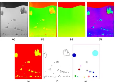
Figure 3.1: (a) An example of an original grayscale input image, (b) the representation of the image by the program after normalization(c) detection of the local average,(d) the original image corrected for inhomogeneous illumination(e)the binary frame result-ing from phase segmentation, (f) edge detection to obtain the circumference of a bubble(g)representation of the equivalent bubble diameter as circles

distribution, which is necessary for reliable phase separation. Note that, on the contrary to most DIA algorithms described in literature, the light source is not behind the bed, but in front of it. The reason is that the DIA program must also be able to process images obtained for PIV analysis and therefore, it is required that the dense phase is illuminated thoroughly.

DIA starts with importing a bitmap (.bmp) image into an intensity matrix Ii,j. Color images are transformed to grayscale, and the intensity of the image is normalized to

0.0 ≤ Ii,j ≤ 1.0. As an example, the photograph shown in figure 3.1a is imported into DIA. For a better visualization, a full color spectrum is assigned to numbers between 0 and 1 (i.e. after normalization), instead of the grayscale spectrum. The result is given in figure3.1b.

The walls of the reactor on the picture are automatically detected or manually assigned, and removed from the image, leaving the bed and freeboard for further analysis. The freeboard above the bed is automatically detected by a discrete edge detection algorithm (see figure3.1c, for further explanation see appendixB). This part of the image will be marked and disregarded in functions calculating the (local) average or normalization. An intensity gradient can be seen in figure 3.1b, caused by inhomogeneous lighting. This effect is removed by subtracting a (semi)-local average from the image, resulting in figure3.1d. Pixels within a predefined rangeraare averaged. See the expression below.

Avgi,j =

Px=i+ra

x=i−ra

Py=j+ra

y=j−raIx,y

r2 a

in which currentlyra is set to:

ra= 0.25Nx (3.1b)

in which i and j are the pixel coordinates and Nx is the image width in pixels. Note that for certain pixels near the edge of the image, it is inevitable that x ory points to a location outside the image borders. Of course, pixels outside the image borders are disregarded. Also, pixels on the freeboard are disregarded in this function.

The final preprocessing step accounts for smoothing the granular phase. The image is blurred using a 5×5 mask. This results in a more uniform phase separation because the edges of particles are filtered out. The histogram of the image is now bimodal due to the preprocessing steps.

Segmentation can take place, using an image dependent threshold T = 0.9× hIi, in which hIi is the average image intensity. Pixel intensities below T represent a bubble and are set to 0, other pixels are set to 1. Different threshold values were tested to obtain the best performance in phase segmentation. The result of phase segmentation is shown in figure3.1e.

The walls of the reactor display a shadow at the walls and bottom, causing these areas to be mistaken as bubbles. A function is implemented to remove these shadows. Now the phase segmentation is completed.

3.2.2

Bubble properties

Obtaining bubble information is performed in a postprocessing step. First, bubbles are numbered by tagging adjacent bubble pixels. By counting the total amount of pixels in a single bubble, the program determines the visible surface area Sb. The equivalent

bubble diameter is then determined by (see e.g. Muddeet al.[25]):

db=p4Sb/π (3.2)

The db can be used to draw equivalent circular bubbles (figure 3.1g). The position of a bubble is placed at its center of gravity. Using consecutive images, the velocity of a bubble can be determined if the bubble is also present on a previous image. Two bubbles on subsequent images are linked if the change in position and size of the bubble fulfills the following criteria: the bubble cannot grow or shrink more than 50% of its original size, and the bubble cannot move more than0.5db. If a bubble breaks up or if bubbles coalesce, the velocity of the new bubbles is set to zero.

The aspect ratio and sphericity of the bubbles are determined as discussed in section 2.3.2. A Sobel edge detection algorithm is used to obtain the bubble edges (figure3.1f), which are equivalent to the perimeter, needed for the sphericity. It was found that a

5×5convolution mask performed much better than a smaller mask.

The final step is to write the data to a text file which is used for further analysis.

3.2.3

Validation of DIA

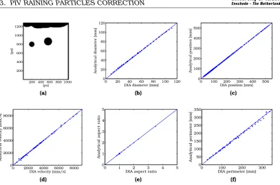
To validate the DIA measurements of bubble size, position, velocity, aspect ratio, perime-ter and the bubble tracking system, four image series were created and imported into DIA. DIA should be able to detect numerous shapes. Circles and rectangles were drawn on the images to verify that these shapes were being detected correctly. For these partic-ular shapes it is easy to obtain the surface area and circumference, needed for further validation.

3.3. PIV RAINING PARTICLES CORRECTION

[px]

[px]

200 400 600 800 1000 200

0 2000 4000 6000 8000 0

Figure 3.2: (a)An example of a synthetic image with known bubble properties to validate DIA. The other images are parity plots:(b)diameter;(c)Bubble position;(d)Bubble veloc-ity;(e)Bubble aspect ratio;(f)Perimeter (circumference).

3.3

PIV Raining Particles Correction

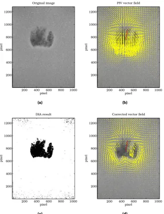
PIV produces instantaneous vector fields, based on the particle movement inside an interrogation zone. PIV however, does not determine how many particles are actually correlated in the interrogation zone, i.e. the amount of particles flowing in that par-ticular interrogation zone. A PIV post processing method is proposed in this section, correcting the original instantaneous PIV flow fields for the amount of particles in this interrogation zone.

For the correction, results of the DIA program (described in section3.2) are used. The program combining called CRiB, which is an acronym for ”Correction for Raining In Bubbles”.

3.3.1

Particle raining

the limits of AVGi,j±2·RMSi,j. However, it is argued that this type of filtering is

uncon-trolled, because the filter only depends on the velocity, and not the amount of particles on which the velocity is based. Therefore, valuable data may be disregarded or, perhaps even worse, erroneous vectors are still taken into account for the time-averaged result.

3.3.2

Correction outline

In order to determine whether a vector must be accounted for in the time-average result, the particle density must be determined for every PIV interrogation zone. Link[15] used a particle detection system to obtain the porosity of a spout-fluid bed using coarse par-ticles. A similar approach is used here, however the used particle type is much smaller. Although the particles on PIV images have to be individually distinguishable, the exact number of particles is hard to determine automatically for small particle systems. One may suggest using the average intensity of an interrogation zone as an estimate for the number of particles in that particular zone. However, a linear relation between the intensity and the packing degree cannot be assumed.

On the contrary, the binary frame provided by DIA can be used to classify every pixel in a single phase (figure3.1e). The frame is denoted as a matrixε∗_i,j, in which 0 represents the bubble phase, and 1 the emulsion phase. (Note that the values ofε∗_i,j are swapped as compared to the conventional porosity εi,j.) The matrix is used as a reference to

determine for every instantaneous vector whether it belongs to the bubble phase, and should thus be disregarded, or to the emulsion phase in which case no correction is needed, or somewhere in between.

This correction algorithm basically assumes that there are no particles present in a bubble. Also, it assumes that the emulsion phase has a constant density.

3.3.3

Correction algorithm

PIV vectors are computed based on an interrogation zone of size N×N pixels. All the pixels in that zone are averaged to obtain the correction factor ε∗ using the DIA infor-mation. The correction factor is multiplied with vectoru:

u∗i,j=ui,j×ε∗i,j (3.3a)

In this equation, u∗

i,j represents the corrected vector, and ui,j the original vector. By

using the average of the entire interrogation zone, vectors based on the bubble-particle interface are still partly considered, whereas the correction factor of an interrogation zone completely within a bubble is set to zero. On the other hand, an interrogation zone consisting of solely emulsion phase pixels leaves the original vector untouched.

Not all vectors on the corrected vector fields should account as a complete vector in the time-averaged result. For instance, imagine a vector based on an interrogation zone with ε∗_i,j = 0 (i.e. a bubble). The corrected velocity for the emulsion phase then gives

u∗

i,j = 0. It is undesired that this velocity is accounted in the time averaged result,

3.3. PIV RAINING PARTICLES CORRECTION

pixel

pixel Original image

200 400 600 800 1000

200 400 600 800 1000 1200

(a)

pixel

pixel PIV vector field

200 400 600 800 1000

200 400 600 800 1000 1200

(b)

pixel

pixel DIA result

200 400 600 800 1000

200 400 600 800 1000 1200

(c)

pixel

pixel Corrected vector field

200 400 600 800 1000

200 400 600 800 1000 1200

(d)

Figure 3.3:The yellow arrows denote particle phase movement. As a reference, the velocity of the bubble (0.34 m/s) is given in red.(a) An image pair of a single bubble is used to perform PIV calculations,(b)gives the PIV velocity vectors for the image pair,(c)

186 188 190 192 194

186 188 190 192 194 114

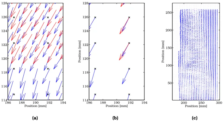
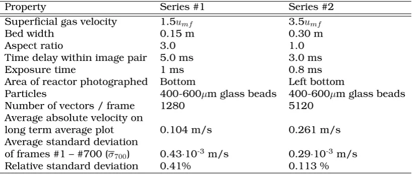
Figure 3.4: (a) A part of the overlap area of two time-averaged PIV sessions. The crosses indi-cate the interpolation grid points.(b)Based on four surrounding points of the same time-averaged vector field, vectors are calculated on the interpolation grid. If an in-terpolated vector can be derived from more than one time-averaged vector field, the resulting vectors are averaged.(c)The combination of two interpolated vector fields. The grid points at the left and top side cannot be calculated with these two time-averaged results.

considered partially in the time-averaged result. Therefore, the corrected time-averaged velocityuon positioni, jover Nf vector fields is calculated by:

u∗i,j=

The Stitch program combines multiple PIV time-averaged flow fields. This is necessary in situations in which the bed cannot be photographed as a whole, due to restrictions on the spatial resolution (see Appendix A). In these cases, PIV image series have to be recorded sequentially of different areas of the bed, which in total cover the full bed area.

Seemless stitching can only be performed when the time-averaged vector fields are fully developed. A new vector grid is created by bilinear interpolation of the original results. Multiple vectors on the interpolated grid, due to overlap of the original series, are averaged.

3.4.1

Outline of the Stitch Program

3.5. VERIFICATION OF IMAGE ACQUISITION SCHEME

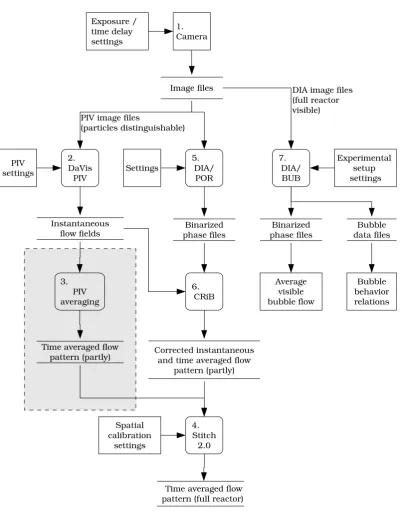
shifting of the camera. Therefore, the stitch program initializes by defining a new grid over the entire bed domain. A part of the overlap area is shown in figure 3.4a, and it can be seen that the two time-averaged results provide their vectors on a different grid. The program uses a bilinear interpolation scheme to derive vectors on the interpo-lated grid. This is performed for all original time-averaged vector plots independently. Overlapping vectors are now defined at the same location on the interpolated grid. Af-ter inAf-terpolation, the program deAf-termines which inAf-terpolation grid vectors are defined more than once (overlap), and averages their velocity components. The new vectors in the overlap area is given in figure 3.4b. Figure 3.4c gives the result of stitching two vector fields.

The result of the Stitch program was validated by synthetic vector plots. Furthermore, it must be mentioned that the bilinear interpolation algorithm used by the stitch pro-gram may not be used to obtain a higher resolution than originally obtained by PIV. Throughout this thesis, the number of vectors was significantly reduced.

3.5

Verification of Image Acquisition scheme

In this research, PIV is performed to obtain a time-averaged flow field of the emul-sion phase. The time-averaged result can be obtained from multiple instantaneous flow fields. These flow fields emerge from PIV image pairs. The Verification of Image Acqui-sition scheme-program (VIA) determines whether the number of image pairs, and timer and shutter settings used for PIV experiments are sufficient to produce reproducible time-averaged results. Basically, the program compares the accumulating average vec-tor length of an increasing number of frames, and compares it to an independently determined long-term average. The emerging instantaneous flow patterns all together must yield a constant time-averaged result, and should not be subject to change when taking more instantaneous flow patterns into account.

3.5.1

Algorithm

Instantaneous vector plots (frames) are obtained from the DaVis program after it has performed the PIV calculations. These files are loaded into a matrix with a size of Ni

frames times Nj vectors (frames are numbered with i, vectors are numbered with j).

The vector length `i,j is calculated with vector components in the x-direction (u) and

z-direction (v):

`i,j=qu2

i,j+v2i,j (3.5)

The accumulating average of the length of vectorjis the average of the length at current frameic, and all preceding frames{ic−1, ic−2, . . . ,1}.

`ic,j =

Pic

i=1`i,j

ic (3.6)

The deviation of this average value `i_c,j from a long term time-average (here denoted

by `∞,j) is used to estimate the reliability of the measurement series. `∞,j should be

measuredindependentlyat identical experimental conditions and over asufficiently long period, it accounts for the ’true’ average velocity for vectors at positionj. The standard deviation of the time average of frames {ic−1, ic−2, . . . ,1} compared to the long-term

average velocity can be defined as:

The program calculates the sum of standard deviations of all vectors in a frameic, and divides it by the number of vectors on that frame (Nj), yielding the average standard deviation up to a frameic.

σi_c=

Nj

X

j=1 σi_c,j

Nj

(3.8)

The program yields a file containingσi_c for alli, which can be plotted as a function of i. Note that this involves the deviation of the vector length, similar to the RMS value, and does not contain information on the direction of the vector.

3.5.2

Example

Two PIV experiments at different conditions were analyzed by the VIA program. In both cases, 4 image series were taken of 700 image pairs each. The superficial gas velocity was set at 1.5umf and 3.5umf. Other parameters can be found in table 3.1. From the

four imaging series, an average of three times 700 instantaneous vector fields was used to obtain the long term average flow pattern, and one series was used to calculate the accumulating average. Image pairs were taken at 4Hz, resulting in a total measurement time of 3 minutes.

It is shown that 700 instantaneous vector fields are yielding accurate time-averaged re-sults with a low standard deviation from the long-term average at different conditions. The evolution of the standard deviation over an increasing number of instantaneous vector plots, is given in figure3.5.

Figure3.5 also gives the deviation from the long-term average of the3.5umf measure-ment series corrected for raining particles. It was shown that the deviation decreases. This confirms the expectations because the relatively large velocity vectors of raining particles are filtered out, hence the vectors taken into account are of more uniform length.

It can be expected that for image series from the top of the bed (i.e. with the freeboard in the field of view), the standard deviation will be higher due to more rigorous particle displacement when a bubble erupts at the surface. For the experiments however, we are not interested in the movement of the particles in the freeboard area. Besides, the fact that the standard deviation does not vary much after a certain amount of images is of more importance than the absolute value of the eventual standard deviation, provided that the standard deviation is of course reasonably low (preferably in the magnitude of mm/s).

3.6

Data Flow Diagram

3.6. DATA FLOW DIAGRAM

Property Series #1 Series #2

Superficial gas velocity 1.5umf 3.5umf

Bed width 0.15 m 0.30 m

Aspect ratio 3.0 1.0

Time delay within image pair 5.0 ms 3.0 ms

Exposure time 1 ms 0.8 ms

Area of reactor photographed Bottom Left bottom

Particles 400-600µm glass beads 400-600µm glass beads

Number of vectors / frame 1280 5120

Average absolute velocity on

long term average plot 0.104 m/s 0.261 m/s

Average standard deviation

of frames #1 – #700 (σ700) 0.43·10-3 m/s 0.29·10-3m/s

Relative standard deviation 0.41% 0.113 %

Table 3.1:Minimum PIV time test parameters

0 100 200 300 400 500 600 700

10−5 10−4 10−3 10−2 10−1

Number of frames i_c

Average standard deviation [m/s]

1.5u_mf 3.5u_mf 3.5u

mf corrected

Figure 3.5:Evolution of the average standard deviation over an increasing number of instanta-neous vector plots taken into account to derive the time-averaged result. The mea-surements were performed atu0= 1.5umf and an aspect ratio of 3 in the 15 cm wide

bed, and3.5umf with an aspect ratio of 0.5 in the 30 cm wide bed, both with glass

beads of sizedp = 400−600µm. Also, the effect of correcting for raining particles is

Exposure / 

3.6. DATA FLOW DIAGRAM

from DaVis program (3), i.e. without correcting for raining particles (gray area). How-ever, this route is not used, as correctionhasto take place on current results.

Chapter 4

Experiments

4.1

Introduction

Experimental data are acquired by photographing a pseudo-2D fluidized bed. The ex-perimental setup will be discussed first in section 4.2.1. Obviously, the camera is an important part of the setup. The settings used for the camera are discussed in section 4.2.2. The images are imported into the appropriate program which performs the calcu-lations. PIV calculations are performed using commercial software. The settings of the PIV software are discussed in section 4.2.3. The glass beads used in the experiments were analyzed. The result is given in section4.2.4. Finally, an overview of the different investigated parameters is given in section4.3.

4.2

Experimental setup

4.2.1

Pseudo-2D fluidized bed

The setup contains two pseudo-2D beds with different bed widths which are operated separately. The wide bed has a width ofdbed=0.30 m, the small bed is 0.15 m wide. In both cases, the depth of the pseudo-2D bed is 0.015 m. The behavior of both phases is observed through the glass front plate.

The fluidizing gas is compressed air from the local air network. A buffer vessel is used to maintain a constant pressure. The gas inflow is supplied to the distributor by two inlets. Both inlet streams are controlled using two parallel mass flow controllers (MFC); for low gas flow rates, the 20 l/min MFCs are used. At higher superficial gas velocities, the 100 l/min MFCs are used. The MFC calibration was verified several times as ex-periments with the setup were spread over time and it was found that the calibration maintained to be valid during the experiments. In all cases, the left and right gas inlet were set at equal gas flow rates. The gas from both inlets is combined in a chamber below the fluidized bed, in which air is pre-distributed over the column width. At the top of this chamber, the distribution plate performs the actual gas distribution over the bed.

4.2. EXPERIMENTAL SETUP

61.2

20  l/min

100  l/min

PIV Computer

Mass flow  controllers Water vessel

Lights Humidity 

meter

Pseudo­2D  fluidized bed Adjustable 

camera setup

High speed  camera

Figure 4.1:A schematic representation of the experimental setup. The gas feed is set by mass flow controllers. The camera is placed in front of the bed and can move parallel to the bed both horizontally and vertically. Direct lighting is required for high quality images.

Accuracy of the gas flow

An error is made in the superficial gas flow due to changes in the environment. A deviation of the air temperature of 2◦_{C is found to cause an error in the gas flow of}

about 0.2%. Moreover, the MFCs can vary unknowingly by 0.1. This causes an error of about 0.3%. In total, the gas flow could therefore deviate by 0.5%.

4.2.2

Camera settings

A LaVision ImagerPro high-speed CCD (charge-coupled device) camera is used to record images from the bed. The camera has a maximum resolution of 1024×1280 pixels and contains 2GB of internal memory. An IEEE 1394 FireWire connection is used for data transfer. The camera shutter is controlled by an oscillator connected to the computer. Motion blurring can be prevented by setting a short exposure time. Consequently, the amount of light that reaches the sensor is reduces. Therefore, two 500 W Halogen lights on each side of the setup are used to illuminate the bed. Also, the aperture of the camera can be used to achieve a high contrast on the images, at the cost of a loss of depth of field.

PIV images

of a pair. Using this scheme, the camera is able to record for 3 minutes. Whether the scheme yields a truthful time-average flow field was investigated in section (3.5).

DIA images

Bubble behavior experiments are recorded from a larger distance, to obtain a full view of the entire bed. Therefore, the CCD sensor size is adjusted to contain solely the bed. By declining the resolution of the sensor, images require less memory and therefore, more images can be recorded. The number of images recorded varies between 1424 images (full sensor utilized) up to over 10000 images. Most series are recorded twice under similar conditions. This data will be used to verify the reproducibility of the results. In order to track bubbles, images are recorded with a uniform time delay rather than in pairs. The time delay was set to 10 ms. A delay of 50 ms causes bubbles to move too far between the images, which caused trouble with the tracking system in the DIA program. Using a delay of 2 ms on the other hand, results in a short total measurement time, which is not desired.

4.2.3

PIV Settings

PIV was performed using the DaVis software from LaVision. Correlation of interrogation windows was performed in multi-pass mode; first, a ballpark estimate is made by an interrogation window of 128×128 pixels. Consequently the window size was decreased to 32×32 pixels with 50% window overlap to obtain the eventual resolution. Spatial cross-correlation patterns (e.g. figure 2.3b) were checked visually in a random way to verify whether the correlation peak RD exceeded the random correlation significantly,

i.e. whether the dislocation could be determined with high precision.

For PIV measurements, the maximum resolution of the camera is used, to cover an area as large as possible whilst keeping particles distinguishable. As stated in the PIV design rules (Appendix A), a single particle has to be represented in diameter by at least 3-4 pixels. Although the photographed area may vary slightly due to repositioning the camera, the recordings generally cover 0.12×0.15 m. The number of image series for a single measurement varies between 1 and 15, depending on the size of the bed. For the wide bed, three image series were recorded in lateral direction and in axial direction, up to five series were required. The small bed could be recorded from wall to wall, but depending on the aspect ratio and superficial gas velocity, several image series above each other were required. The image series were recorded with an overlap area of at least 0.02 m. After correction for the overlap of image series, a single vector field attributes approximately 58×74 vectors to the whole flow field.

4.2.4

Particles

The particles used in the experiments are glass beads, considered as model-particles. The density of the particles isρglass= 2500kg m-3_{, which indicates that a particle size as}

low as∼100µm could be chosen to remain in the Geldart B range (figure2.2.1). Due to the fact that PIV images should encapsulate a single particle in at least 3–4 pixels (see appendixA), a diameter range of400 ≤dp ≤600 µm is chosen. Particles in olefin poly-merization reactors range from 0.25-1mm[1]_{, and therefore these particles are within}

the range of the project scope.

The glass beads are produced by SiLibeads, with an indicated particle diameter range from 0.4 to 0.6 mm. This was verified by laser diffraction, using a Sympatec HELOS system. A cumulative distribution function shows the diameter of two samples in figure 4.2a. It is found that the average diameter is about 485µm.

4.3. SUMMARY OF OPERATING CONDITIONS

300 400 500 600 700 0

Superficial gas velocity [m/s]

Pressure drop [mmH

2

O]

(b)

Figure 4.2: (a)Cumulative distribution function of the particle diameter of two samples analyzed by laser diffraction. The markers denote the actual measurements. It can be found that the average diameter is about 480 - 490µm. (b) Experimental determination ofumf by pressur