Acute Myelogenous Leukemia Detection in Blood Microscopic Images
using Different Wavelet Family Techniques
B.k.Lakshmikanth
1, Dr.P.Abdul khayum., M.Tech.,Phd
21
PG Student, Department of ECE, G. Pulla Reddy Engineering College (Autonomous), Kurnool, AP, India
2Professor, Department of ECE, G. Pulla Reddy Engineering College (Autonomous), Kurnool, AP, India
---***---Abstract:
Image segmentation is considered the most critical step in image processing and helps to analyze, infer and make decisions especially in the medical field. Analyzing digital microscope images for earlier Acute Myelogenous leukemia (AML) diagnosis and treatment require sophisticated software and hardware systems. The need for automation of leukemia detection arises since current methods involve manual examination of the blood smear as the first step toward diagnosis. In this paper presents selected mathematical methods used for image segmentation and application of wavelet transform for the following segments classification by multiresolution decomposition of segments blood cell images. The Haar wavelets transform and Daubechies wavelet transform approaches has been adopted here and used for feature extraction allowing its use for image denoising and resolution enhancement as well. Feature classification is then achieved by self-organizing neural networks .A proposed method has been verified for simulated structures and then gives the better segmentation accuracy and Precision for analysis of microscopic images
Keywords- Acute Myelogenous leukemia(AML),Wavelet Transform, Haar Wavelet Transform, Daubechies Wavelet Transform, Feature Extraction, Neural Network, Accuracy and Precision.
I. INTRODUCTION
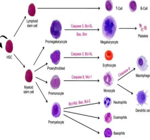
Hematopoiesis is the deterministic process of blood cell formation taking place in the bone marrow [1]. Mature blood cells are produced by a tightly controlled mechanism from hematopoietic stem cells (HSCs) residing in the bone marrow. The distinct leukocytes comprising granulocytes, monocytes, macrophages, natural killer cells and lymphocytes are
essential for the defense against pathogens and foreign invaders, erythrocytes play a pivotal role in the transportation of oxygen to remote organs, and platelets confer the process of blood clotting.
Figure 1: Hematopoiesis
Leukemia is a type of cancer caused by abnormal increase of the white blood cells. According to [1] leukemia can be classified into acute and chronic. Acute leukemia spreads very rapidly and has to be treated promptly rather than chronic leukemia that does not have to be treated promptly. Acute leukemia can be either lymphoblastic (ALL) or myelogenous (AML), based on affected cell type. Chronic leukemia can be either lymphoblastic (CLL) or myelogenous (CML). Acute Myelogenous leukemia (AML) is considered the prime focus of this work, which has a higher expectation of survival rate compared to ALL.
The focus of this thesis is primarily set on the genetic and epigenetic delineation of AML pathogenesis. AML is characterized by the accumulation of immature hematopoietic cells of the myeloid family in the bone marrow lacking the ability to differentiate towards functional granulocytes or monocytes and in rare cases also affecting the development of erythrocytes and megakaryocytes. The term AML specifies a broad spectrum of haematological malignancies and could be considered heterogeneous evidenced by the multitude of underlying abnormalities conferring variegated projection and response to therapy.
Figure 2:Acute Myelogenous leukaemia
AML is a heterogeneous disease with an incidence of approximately 3.8 cases per 100.000 individuals per year with a median age of 70 at presentation.13 Additionally, myelodysplastic syndrome (MDS)18 and myeloproliferative neoplasm (MPN) 19 are pre-leukemic disease entities which can progress towards AML. The first clinical symptoms observed at AML on set are infections, fatigue, haemorrhage and more rarely extra medullary involvement such as gingival hyperplasia, i.e., abnormal increased size of the gum, in cases of acute myelomonocytic or monoblastic leukemia. 20 The symptoms are the result of impaired normal haematopoiesis due to the accumulation of leukemic blasts in the bone marrow, precluding the production of functional mature blood cells. The dysfunction and abnormal distribution of malignant blood cells could readily explain the symptoms; infections (lack of granulocytes), fatigue (lack of erythrocytes), haemorrhage (lack of platelets), gingival hyperplasia (infiltration of malignant blood cells).
1.2. Mutational Landscape and Patterns In AML
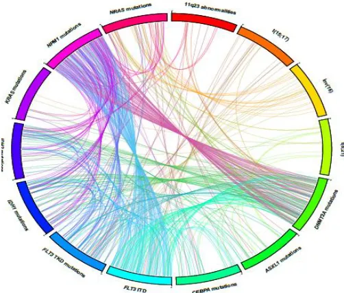
The initiation of AML is not conferred by a single aberration as observed in the core binding factor (CBF) leukaemia’s i.e. AML with chromosomal abnormalities [2]. Detailed studies have demonstrated that combinations of genetic alterations are necessary for the development of explicit leukaemia. These genetic grazes can be dichotomized on size, e.g., large cytogenetic events (translocation, inversions, duplications, deletions, and amplifications), and small genetic lesions (mutations and small insertions and deletions). These combinatorial mutational patterns reflect the heterogeneous nature of AML (Figure 3).
Figure 3: Molecular heterogeneity of AML
thresholding were employed to segment WBCs from the blood smear image. The work in [13] employed contour signature to identify the irregularities in the nucleus boundary. The work in [14] employed selective filtering to segment leukocytes from the other blood components. A watershed segmentation algorithm to segment nucleus from the surrounding cytoplasm of cervical cancer images was proposed by Nallaperumal and Krishnaveni [15]. The work in [16] presented an unsupervised color segmentation to bring out the WBCs from acute leukemia images.
This paper is structured as follows. Section II focuses in detail on the process overview of the existing method. The proposed Daubechies and Haar Wavelet Decompositions method is detailed in Section III. Sections IV present the experimental results of the classifier system based on the features extracted. Section V contains conclusions and future work.
II. EXISTING METHOD
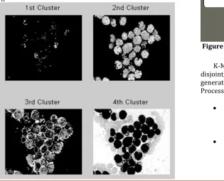
2.1. K-means Cluster Segmentation
Clustering algorithms essentially perform the same function as classifier methods without the use of training data. Thus, they are termed unsupervised methods. In order to compensate for the lack of training data, clustering methods iterate between segmenting the image and characterizing the properties of the each class. In a sense, clustering methods train themselves using the available data. Three commonly used clustering algorithms are the K-means or ISODATA algorithm, the fuzzy c-means algorithm, and the expectation-maximization (EM) algorithm.
Figure 4: K-means Cluster Image (K=4)
The K-means clustering algorithm clusters data by iteratively computing a mean intensity for each class and segmenting the image by classifying each pixel in the class with the closest mean. The number of classes was assumed to be three, representing (from dark gray to white) cerebrospinal fluid, gray matter, and white matter. The fuzzy c-means algorithm generalizes the K-means algorithm, allowing for soft segmentations based on fuzzy set theory. The EM algorithm applies the same clustering principles with the underlying assumption that the data follows a Gaussian mixture model. It iterates between computing the posterior probabilities and computing maximum likelihood estimates of the means, covariances, and mixing coefficients of the mixture model. Although clustering algorithms do not require training data, they do require an initial segmentation (or equivalently, initial parameters). The EM algorithm has demonstrated greater sensitivity to initialization than the K-means or fuzzy c-means algorithms. Work on improving the robustness of clustering algorithms to intensity in homogeneities in MR images has demonstrated excellent success.
Figure 5: Block Diagram of K-means Cluster Classification
K-Means clustering generates a specific number of disjoint, flat (non-hierarchical) clusters. It is well suited to generating globular clusters. Thus the K-Means Algorithm Process in very shortly
The dataset is partitioned into K clusters and the data points are randomly assigned to the clusters resulting in clusters that have roughly the same number of data points,
If the data point is closest to its own cluster, leave it where it is and if the data point is
not closest
to its own cluster, move it into the closest cluster,
Repeat the above step until a complete pass through all the data points’ results in no data point moving from one cluster to another. At this point the clusters are stable and the clustering process ends,
The choice of initial partition can greatly affect the final clusters that result, in terms of inter-cluster and intra-cluster distances and cohesion.
The algorithm assumes that the data features form a vector space and tries to find natural clustering in them. The points are clustered around cancroids µ𝑖∀𝑖=
1 … . 𝑘which are obtained by minimizing the objective. V=∑𝑘
𝑖=1 ∑𝑥𝑗€𝑠𝑖(𝑥𝑖−µ𝑖)2
Where there are k clusters Si, i = 1,2, ……, k and is the cancroids or mean point 𝑥𝑗€𝑠𝑖of all the points .
K-means fairly simple to implement and image segmentation are impressive. As can be seen by the results, the number of partitions used in the segmentation has a very large effect on the output. The algorithm also runs quickly enough that real-time image segmentation could be done with the K-Means algorithm
Figure 6: AML Classification of Existing Method
III. PROPOSED METHOD
In this paper The Discrete Wavelet Transform (DWT) techniques are used .i.e. Haar wavelet transform
and Daubechies wavelet transform approaches has been adopted here.
3.1. Discrete Wavelet Transform
The wavelet transform (WT) has gained widespread acceptance in signal processing and image compression. Because of their inherent multi-resolution nature, wavelet-coding schemes are especially suitable for applications where scalability and tolerable degradation are important. Wavelet transform decomposes a signal into a set of basis functions. These basis functions are called wavelets. Wavelets are obtained from a single prototype wavelet y (t) called mother wavelet by dilations and shifting:
Where a is the scaling parameter and b is the
shifting parameter
Figure 7: 1D- Discrete Wavelet Transform Image
columns. The lowest resolution level LL consists of the approximation part of the original image. The remaining three resolution levels consist of the detail parts and give the vertical high (LH), horizontal high (HL) and high (HH) frequencies. Figure shows 1D-wavelet decomposition of an image.
3.2. Project Implementation
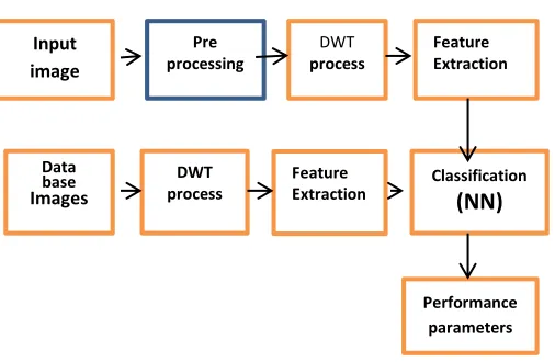
Figure 8: AML Classification of Proposed Method
3.2.1. Image Acquisition
The first stage of any vision system is the image acquisition stage. Image acquisition in image processing can be broadly defined as the action of retrieving an image from some source, usually a hardware-based source, so it can be passed through whatever processes need to occur afterward. Performing image acquisition in image processing is always the first step in the workflow sequence because, without an image, no processing is possible. The image that is acquired is completely unprocessed and is the result of whatever hardware was used to generate it, which can be very important in some fields to have a consistent baseline from which to work. One of the forms of image acquisition in image processing is known as real-time image acquisition. This usually involves retrieving images from a source that is automatically capturing images. Real-time image acquisition creates a stream of files that can be automatically processed.in pre-processing stage sum noise is occurred. So that noise can be removed by using median filter
3.2.2. Haar wavelet Process
The first DWT was invented by Hungarian mathematician Alfredhaar. For an input represented by a
list of numbers, the Haar wavelet transform may be considered to pair up input values, storing the difference and passing the sum. This process is repeated recursively, pairing up the sums to provide the next scale, which leads to differences and a final sum. The Haar wavelet is also the simplest possible wavelet. The technical advantage of the Haar wavelet is of signals with sudden transitions, such as monitoring of tool failure in machines.
Figure 9: Sub band Representation in Haar wavelet Transform
The Haar wavelet's mother wavelet
function can be described as
Its scaling function can be described as
Input image
Pre processing
DWT process
Feature Extraction
Extracti
on
Database
Images
DWT process
Feature
Extraction Classification
(NN)
Figure 10: AML Sub bands for Haar wavelet Method
3.2.3. Daubechies Wavelet Process
The Daubechies wavelets, based on the work of Ingrid Daubechies, are a family of wavelets defining a discrete wavelet transform and characterized by a maximal number of vanishing moments for some given support. With each wavelet type of this class, there is a scaling function (called the father wavelet) which generates an orthogonal multiresolution analysis.
The Daubechies D4 transform has four wavelet and scaling function coefficients. The scaling function coefficients are
ℎ
0=
1+√34√2ℎ
1=
3+√34√2ℎ
2=
3−√34√2
ℎ
3=
1−√34√2Each step of the wavelet transform applies the scaling function to the the data input. If the original data set has N values, the scaling function will be applied in the wavelet transform step to calculate N/2 smoothed values. In the ordered wavelet transform the smoothed values are stored in the lower half of the N element input vector. The wavelet function coefficient values are:
G0=h3 G1=-h2 G2=h1 G3=-h0
Each step of the wavelet transform applies the wavelet function to the input data. If the original data set has N values, the wavelet function will be applied to calculate N/2 differences (reflecting change in the data). In the ordered wavelet transform the wavelet values are stored in the upper half ofthe N element input vector.
The scaling and wavelet functions are calculated by taking the inner product of the coefficients and four data values. The equations are shown below.
Daubechies D4 scaling functions:
𝑎𝑖= ℎ0𝑠2𝑖+ ℎ1𝑠2𝑖+1+ ℎ2𝑠2𝑖+2+ ℎ3𝑠2𝑖+3
a[i]= ℎ0s[2i]+ℎ1s[2i+1]+ℎ2s[2i+2]+ℎ3s[2i+3];
Daubechies D4 wavelet function:
𝑐𝑖= 𝑔0𝑠2𝑖+ 𝑔1𝑠2𝑖+1+ 𝑔2𝑠2𝑖+2+ 𝑔3𝑠2𝑖+3
Figure 11: Signal Representation in Daubechies wavelets
Transform
Each Iteration in the wavelet transform step calculates a scaling function value and a wavelet function value. The index i is incremented by two with each iteration, and new scaling and wavelet function values are calculated.
Figure 12: AML Sub bands for Daubechies wavelet Method
3.2.4. Features Extraction
Feature Extraction starts from an initial set of measured data and builds derived values (features) intended to be informative, non-redundant, facilitating the subsequent learning and generalization steps, in some cases leading to better human interpretations. Feature extraction is related to dimensionality reduction. When the input data to an algorithm is too large to be processed and it is suspected to be redundant (e.g. the same measurement in both feet and meters, or the repetitiveness of images presented as pixels), then it can be transformed into a reduced set of features (also named features vector). This process is called feature extraction. The extracted features are expected to contain the relevant information from the input data, so that the desired task can be performed by using this reduced representation instead of the complete initial data.
Feature extraction involves reducing the amount of resources required to describe a large set of data. When performing analysis of complex data one of the major
problems stems from the number of variables involved. Analysis with a large number of variables generally requires a large amount of memory and computation power or a classification algorithm which over fits the training sample and generalizes poorly to new samples. Feature extraction is a general term for methods of constructing combinations of the variables to get around these problems while still describing the data with sufficient accuracy. For example; with an 8 grey-level image representation and a vector t that considers only one neighbour, we would find; Entropy, Energy, Contrast, Correlation Coefficient and Homogeneity.
Local Binary Pattern: The concept of Local Binary Patterns
(LBP) was introduced for texture classification. The LBP combines the structural and statistical image analysis approaches into a single high efficiency transformation which is invariant with respect to monotonic gray scale transformations and scaling. In the LBP method each pixel is replaced by a binary pattern which is derived from the pixel's neighbourhood. Each gray scale pixel P of an image is used as a centre of a circle with radius r. The number of samples M determines the amount of points that are taken uniformly from the contour of the circle. These points are interpolated from adjacent pixels if needed. The sample points are compared against the pixel P one by one with a simple comparison operation which result a binary zero if the centre point is larger than the current sample point and one otherwise. When doing this operation for example clockwise from a certain starting point the result will be a binary pattern with length M. [4]3.2.5. Training Process
3.2.5.1. Neural Network
The first artificial neuron was produced in 1943 by the neurophysiologist Warren McCulloch and the logician Walter Pits. An Artificial Neural Network (ANN) is an information processing paradigm that is inspired by the way biological nervous systems, such as the brain, process information. The key element of this paradigm is the novel structure of the information processing system. It is composed of a large number of highly interconnected processing elements (neurons) working in unison to solve specific problems. ANNs, like people, learn by example. An ANN is configured for a specific application, such as pattern recognition or data classification, through a learning process. Learning in biological systems involves adjustments to the synaptic connections that exist between the neurons.
complex to be noticed by either humans or other computer techniques. A trained neural network can be thought of as an "expert" in the category of information it has been given to analyse. This expert can then be used to provide projections given new situations of interest and answer "what if" questions.
Figure 13: Architecture of Neural Network
Finally NN can be classified AML is normal or AML is
abnormal
IV. EXPERIMENTAL RESULTS
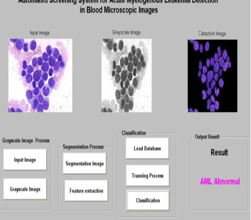
Results of a selected part of the real image representing the microscopic image of crystals are presented in Figure. Image segmentation using wavelet transform is able to detect most of image segments even though the problem of fault class boundaries can arise in some cases.
Figure14: AML Classification of Proposed Method
Performance Evaluation:
In the proposed method the performance evaluation is done through statistical analysis, for this first calculate True Positive, False Positive, False Negative and True Negative. From this, Sensitivity, Specificity, Accuracy, Precision and F-measure are calculated.
Sensitivity=TP/ (TP+FN)
Specificity=TN/ (TN+FP)
Accuracy= (TP+TN)/ (TP+FP+TN+FN)
Precision=TP/ (TP+FP)
F-measure= (2* Precision* Sensitivity) /
(Precision + Sensitivity)
Performance
parameters
LBP WITH
OUT LBP
Kmeans+DWT
Sensitivity 95.19 99.94 60
Specificity 84.19 76.03 50
Accuracy 97.48 76.04 50.0998
Precision 93.7 76.06 11.95
F-measure .944 .8638 2.34375
Table 1:Comparision Table for Existing and Proposed
Bargraph of various parameters for existing and proposed
methods
Bargraph of various parameters for existing and proposed
methods
V. CONCLUSION:
The paper presents some possibilities of image segmentation and classification using wavelet transform. It
is possible to summarize that wavelet transform provide many possibilities of detection of image segment features owing to its multiresolution properties and the possibility to choose different wavelet functions(Haar wavelets and Daubechies wavelet) appropriate for a given problem as well. Segments boundary signals were used for image classification even though there it is possible to use two dimensional wavelet transform for detection of patterns of individual segments texture, two. Methods discussed in the paper have been applied to analysis of shapes of microscopic images of crystals. Similar methods can be used in other applications in a wide range of interdisciplinary problems of texture analysis including biomedical imaging, processing of satellite images, communications and remote earth observations.
Future Work:
The future work can be implement with other algorithms related to this process when perceive used methodologies have some constraints. Further research will focus on collection of more samples to yield better performance and building an overall system for cancer classification
References:
[1]. G.. C.C.Lim, "Overview of Cancer in Malaysia," Japanese Jomal of Clinical Oncology, Department of Radiotherapy and Oncology, Hospital Kuala Lumpur, 2002.
[2].Golub TR, Slonim DK, Tamayo P, et al. Molecular classification of cancer: class discovery and class prediction by gene expression monitoring. Science. 1999;286(5439):531-537.
[3].F. Scotti, “Automatic morphological analysis for acute leukemia identification in peripheral blood microscope images,” in Proc. CIMSA, 2005, pp. 96–101.
[4].Q. Liao and Y. Deng, “An accurate segmentation method for white blood cell images,” in Proc. IEEE Int. Symp. Biomed. Imaging, Atlanta, GA, USA, 2002, pp. 245–248. [5].P. Bamford and B. Lovell, “Method for accurate unsupervised cell nucleus segmentation,” in Proc. Eng. Med. Biol. Soc. Conf., 2001, vol. 3, pp. 2704–2708.
[6].N. Sinha and A. G. Ramakrishnan, “Blood cell segmentation using EM algorithm,” in Proc. 3rd Indian Conf. Compute. Vis., Graph., 2002, pp. 445–450.
[7].R. D. Labati, V. Piuri, and F. Scotti, “ALL-IDB: The acute lymphoblastic leukemia image database for image processing,” in Proc. IEEE ICIP, Brussels, Belgium, Sep. 11– 14, 2011, pp. 2045–2048.
[8].M. Sezgin and B. Sankur, “Survey over image thresholding techniques and quantitative performance
0 20 40 60 80 100 120
SensitivitySpecificity Accuracy Precision FMeasure
evaluation,” J. Electron. Imaging, vol. 13, no. 1, pp. 146–165, Jan. 2004.
[9].K. Nallaperumal and K. Krishnaveni, “Watershed segmentation of cervical images using multiscale morphological gradient and HSI color space,” Int. J. Imaging Sci. Eng., vol. 2, no. 2, pp. 212–216, Apr. 2008.
[10].R. Adollah, M. Mashor, N. Nasir, H. Rosline, H. Mahsin, and H. Adilah, “Blood cell image segmentation: A review,” in Proc. IFMBE. Berlin, Germany: Springer-Verlag, 2008, ch. 39, pp. 141–144.
[11].F. Scotti, “Robust segmentation and measurement techniques of white cells in blood microscope images,” in Proc. IEEE Conf. Instrum. Meas. Technol., 2006, pp. 43–48. [12].C. C. Chang and C. J. Lin, “LIBSVM: A library for support vector machines,” ACM Trans. Intell. Syst. Technol., vol. 2, no. 3, p. 27, Apr. 2011.
[13].S. Mohapatra, D. Patra, and S. Satpathi, “Image analysis of blood microscopic images for acute leukemia detection,” in Proc. IECR, 2010, pp. 215–219.
[14].S. Mohapatra, S. Samanta, D. Patra, and S. Satpathi, “Fuzzy based blood image segmentation for automated leukemia detection,” in Proc.ICDeCom, 2011, pp. 1–5. [15]. S. Mohapatra, D. Patra, and S. Satpathi, “Automated cell nucleus segmentation and acute leukemia detection in blood microscopic images,” in Proc. ICSMB, 2010, pp. 49–54. [16]. R. Rangayyan, Biomedical Image Analysis. Series Title: Biomedical Engineering. Boca Raton, FL, USA: CRC Press, Dec. 2004.