Speed Control of Servo Motor Using Optimized Artificial Multilayer Neural Network Based PID Controller

Speed Control of Servo Motor Using

Optimized Artificial Multilayer Neural

Network Based PID Controller

Lalithamma GA1, Dr.P.S. Puttaswamy2

Associate Professor, Dept. of E&E, SJBIT, Bangalore, India1

Professor, Dept. of E&E, PESCE, Mandya, India2

ABSTRACT: The DC servo motors are extensively used in the industries. Due to overhead of maintaining is high for DC servo motors the trend is switching towards AC servo motors. The AC servo motors plays a important role in industries for driving the motors and its applications can be extended to drive the wheels of the robots, caterpillars etc. the controller is essential to make the decisions when there is variations in the parameters like friction, required amount of torque to drive the load etc. The centre of attention of the research is to design the direct torque (DTC) control paradigm using Artificial Neural Network, it contains many hidden layer to provide the efficient results for variations in the parameters and speed. The results are simulated in the Mat lab, Simulink and compared the results with different algorithm. It shows that neural network is able to enhance the speed of the motors for various load conditions. This system can be adopted in robotic industries and various other fields to take decisions on its own to drive the motor for different speed.

KEYWORDS:AC servo motor, neural network, parameter variations, direct torque control.

I. INTRODUCTION

PID Controller is a general control loop feedback mechanism (controller) widely used in industrial control systems. PID

controller when used improves overall time response of the system. Controller is an element which accepts the error in

some form and decides the proper corrective action. The controller is the heart of the control system. The accuracy of the entire control system depends on the sensitive of controller to the error detected and the action for those errors. Before incorporating any controllers to the system tuning to the required machine is essential, mainly to operate in specified mode. The instructions followed in tuning the controller to the system will vary, few methods follow mathematical models, error and trial methods etc. but these possess own advantage and disadvantages therefore the solution to this problem is through coding i.e. software structure are imposed on the PID tuning for excellent controlling. There are two types of controller namely continuous and discontinuous controllers the main difference between two are the continuous controllers vary its output smoothly in accordance with the error occurred in the system.

The continuous controller has three types

P-Proportional control mode: The output of the Proportional control models simple and proportional to the error e(t). I-Integral Control mode:In Integral mode the value of the controller output P(t) is changed at a rate which is

proportional to the actuating error signal e(t).

D-Differential control mode:In Derivative mode the error is a function of time and at a particular instant it can be zero.

wavelet based Elman neural network, they worked on improving the tracking performance. The approximate error is determined by using the adaptive bound estimation algorithm. [2] The result is simulated using the Mat lab and it clearly shows that controller works efficiently during the non-linear conditions.

Lalithamma.G.A has presented a method to control the servo motor using PID controlling, tuning the controller using the neural network. This paper extends the work presented in [4] and presents a methodology called as direct torque (DTC) control paradigm using the neural network is developed for optimal speed control in servo motors. In the research work the predominant emphasis has been made on studying and developing different neural network algorithms and their suitability for servo controls applications. Ultimately a Multi-Layer Artificial Neural Networks (ANN) system has been designed and trained for modeling the plant parameter variations. Enhancements in the speed control performance have been presented for smaller variations and larger variations in the motor parameters and the load conditions. [4] The real-time plant’s properties are unpredictable, unable to provide the accurate control lines to the plant which in-turn decreases the performance. [5]

II. ARTIFICIAL NEURAL NETWORK

By the literature survey it is clear that the ANN will provide better results for designing the controller. The ANN will select the optimum solution to the specified case, the tuning of the controller is performed by hidden layer and the decision is pushed to PID. The application of the neural network is vast used to determine the operation point, efficient power factor in electrical field and in image processing it is used for identifying the tumors, veins, texture, object detection and still more.

ANN is the type of machine learning process, the developer will extract the features and fed to the system through the labels. Due to this property the ANN can be applied in the field of object count, medical applications, biometric security system, voice controlled devices etc. During the training phase the weights are provided to the hidden layer according to standards defined from users. This process is repeated till the tested samples are matched with the pre-defined input sets. Neural network based PID controller implementation and its computational task involved is so small that the on line adaptation becomes easy.

The Fig1 shows the general training structure of the ANN.

Fig.1. Training Structure of the ANN System

The weight of the network is assigned for input to hidden layer, and furthermore, hidden to output later. From the input

layer to hidden layer weights are denoted as













The hidden layer to output layers weights are represented as





2.1 Neural Network Architecture

Fig 2: Multi-layer neural network architecture

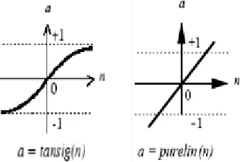
Fig 3: Neuron Model, single input and multi input neurons

Fig 4: Neuron transfer functions, hyperbolic tangent sigmoid (left) and pure linear (right)

2.2 Neural Network Algorithms

This section discusses some of the neural network algorithms used for the training of the designed neural network.

2.2.1 Levenberg-Marquardt algorithm

This algorithm was designed to approach second order training speed without having to compute the Hessian matrix [8]. When the performance function has the form of a sun of squares, then the Hessian matrix can be approximated as: H=JTJ (1)

And the gradient can be computed as:

G=JTe (2)

matrix in the following update:

Xk+1=Xk-[JT+uI]-1JTe (3)

When the scalar μ is zero, this is the Newton’s method using the approximate Hessian matrix. When μ is large, it becomes the gradient descent with a small step-size. The scalar μ is decreased after each successful step and is increased only when a tentative step would increase the performance function. Hence the performance function is always reduced at each iteration [9].

2.2.2 Bayesian regulation back-propagation

It updates the weight and bias values according to Levenberg-Marquardt optimization [9]. It minimizes a combination of squared errors and weights, and then determines the correct combination so as to produce a network that generalizes well. The process is called Bayesian regularization. Bayesian regularization minimizes a linear combination of squared errors and weights. It also modifies the linear combination so that at the end of training the resulting network has good generalization qualities. This Bayesian regularization takes place within the Levenberg-Marquardt algorithm.

2.2.2 Bayesian regulation back-propagation

It updates the weight and bias values according to Levenberg-Marquardt optimization [9]. It minimizes a combination of squared errors and weights, and then determines the correct combination so as to produce a network that generalizes well. The process is called Bayesian regularization. Bayesian regularization minimizes a linear combination of squared errors and weights. It also modifies the linear combination so that at the end of training the resulting network has good generalization qualities. This Bayesian regularization takes place within the Levenberg-Marquardt algorithm.

2.2.3 Cyclic Order Training

This algorithm trains a network with weight and bias learning rules with incremental updates after each presentation of an input. Inputs are presented in cyclic order. For each epoch, each vector (or sequence) is presented in order to the network with the weight and bias values updated accordingly after each individual presentation.

2.2.4 BFGS quasi-Newton back-propagation

Newton's method is an alternative to the conjugate gradient methods for fast optimization. The basic step of Newton's method is: Xk+1=Xk-Ak-1gk (4)

Where, A-1k the Hessian matrix (second derivatives) of the performance index at the current values of the weights and biases .

Newton's method often converges faster than conjugate gradient methods. Unfortunately, it is complex and expensive to compute the Hessian matrix for feed forward neural networks. There is a class of algorithms that is based on Newton's method, but which does not require calculation of second derivatives. These are called quasi-Newton (or secant) methods. They update an approximate Hessian matrix at each iteration of the algorithm. The update is computed as a function of the gradient. The quasi-Newton method that has been most successful in published studies is the Broyden, Fletcher, Goldfarb, and Shanno (BFGS) update. This algorithm requires more computation in each iteration and more storage than the conjugate gradient methods, although it generally converges in fewer iterations. The approximate Hessian must be stored, and its dimension is n x n, where n is equal to the number of weights and biases in the network.

2.2.5 Conjugate gradient algorithm

In basic back-propagation algorithm, weights are adjusted in the steepest descent direction. In the conjugate gradient algorithm, a search is performed in conjugate directions providing a faster convergence. In most of the conjugate gradient algorithms, the step size is adjusted at every iteration. All conjugate gradient algorithms start by searching in the steepest descent direction in first iteration and then perform a line search to determine the optimal distance to move along the current search direction. The next search direction is determined such that it is conjugate to previous search directions.

2.2.6 Resilient back-propagation algorithm

The use of sigmoid function in the hidden layers causes a problem in using the steepest descent to train a multilayer network. The resilient back-propagation training algorithm eliminates these effects of magnitude of the partial derivatives. The derivative sign determines the direction of the weight update. The update value of each weight and bias is increased by a factor whenever the derivative of the performance function has the same sign for two successiveiterations. The update value is decreased by a factor whenever the derivative with respect to weight changes sign from the previous iteration. The update value does not change if the derivative is zero.

2.2.7 One step secant back-propagation

requires slightly more storage and computation per epoch than the conjugate gradient algorithms. It can be considered a compromise between full quasi-Newton algorithms and conjugate gradient algorithms.

2.2.8 Scaled conjugate gradient back-propagation

This algorithm updates weight and bias values according to the scaled conjugate gradient method but does not perform a line search at each iteration.

2.2.9ABC

Artificial bee colony (ABC) algorithm is a recently proposed optimization technique which simulates the intelligent foraging behaviour of honey bees. A set of honey bees is called swarm which can successfully accomplish tasks through social cooperation. In the ABC algorithm, there are three types of bees: employed bees, onlooker bees, and scout bees. The employed bees search food around the food source in their memory; meanwhile they share the information of these food sources to the onlooker bees. The onlooker bees tend to select good food sources from those found by the employed bees. The food source that has higher quality (fitness) will have a large chance to be selected by the onlooker bees than the one of lower quality. The scout bees are translated from a few employed bees, which abandon their food sources and search new ones.

In the ABC algorithm, the first half of the swarm consists of employed bees, and the second half constitutes the onlooker bees.

The number of employed bees or the onlooker bees is equal to the number of solutions in the swarm. The ABC generates a randomly distributed initial population of SN solutions (food sources), where denotes the swarm size.

Let represent the solution in the swarm, Where is the dimension

size. Each employed bee generates a new candidate solution in the neighborhood of its present position as equation below:

Where

is a randomly selected candidate solution ( ),   is a random dimension index selected from the set 

, and is a random number within . Once the new candidate solution is generated,

a greedy selection is used. If the fitness value of is better than that of its parent , then update with ; otherwise keep unchangeable. After all employed bees complete the search process; they share the information of their food sources with the onlooker bees through waggle dances. An onlooker bee evaluates the nectar information taken from all employed bees and chooses a food source with a probability related to its nectar amount. This probabilistic selection is really a roulette wheel selection mechanism which is described as equation below:

Where is the fitness value of the solution in the swarm. As seen, the better the solution , the higher the

probability of the food source selected. If a position cannot be improved over a predefined number (called limit) of cycles, then the food source is abandoned. Assume that the abandoned source is , and then the scout bee discovers a

new food source to be replaced with as equation below:

Where is a random number within based on a normal distribution and , are lower and

upper boundaries of the dimension. 2.2.10 Back propagation

Backpropagation, an abbreviation for "backward propagation of errors", is a common method of training artificial neural networks used in conjunction with an optimization method such as gradient descent. The method calculates the gradient of a loss function with respect to all the weights in the network. The gradient is fed to the optimization method which in turn uses it to update the weights, in an attempt to minimize the loss function.

networks, made possible by using the chain rule to iteratively compute gradients for each layer. Backpropagation requires that the activation function used by the artificial neurons (or "nodes") be differentiable.

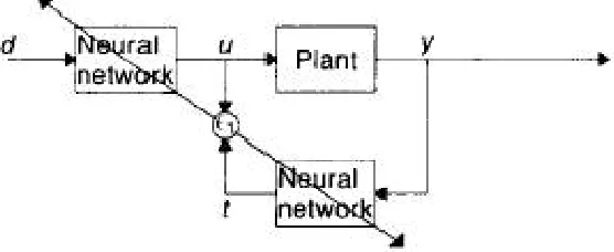
The Fig 5 illustrates the feed forward controller, implemented as neural network architecture, with its output U

driving the plant. The desired response of the plant is denoted by dandy its actual output by y.

Fig 5 Indirect learning architecture.

The neural controller should act as the inverse of the plant, producing from the desired response d a signal U that drives the output of the plant to y = d. The goal of the learning procedure, therefore, is to select the values of the weights of the network so that it produces the correct d - U mappings at least over the range of d's in which we plan to operate the plant.

Suppose that the feed forward controller is successfully trained so that the plant output y=d. Then the network used as the feed forward controller will approximately reproduce the plant input from y (i.e., t=U). Thus, training of the network by adapting its weights might be considered to minimize the error = U - t using the architecture as illustrated above, because, if the overall error E = d - y goes to zero, so does c l. The positive features of this arrangement would be the fact that the network can be trained only in the region of interest since it is started with the desired response d and all other signals are generated from it. Here it can be analysed that it is advantageous to adapt the weights in order to minimize the error directly at the output of the network. Unfortunately, this method, as described, is not a valid training procedure because minimizing cl does not necessarily minimize E. For instance, simulations with a simple plant showed that the network tends to settle to a solution that maps all d's to a single U = uo, which, in turn, is mapped by the plant to t = U for which E, is zero but obviously E is not. This training method remains interesting, however, because it could be used in conjunction with one of the procedures described below that minimize E.

III. SPECIALIZED LEARNING ARCHITECTURE

The Fig 6 represents a specialized learning architecture for training the neural controller to operate properly in regions of specialization only. Here the training involves using the desired response, d, as input to the network. The network has been trained to find the plant input, U that drives the system output, y , to the desired d. This has been accomplished by using the error between the desired and actual responses of the plant to adjust the weights of the network using a steepest descent procedure; during each iteration the weights are adjusted to maximally decrease the error. This procedure requires knowledge of the Jacobian of the plant.

Fig 6 Specialized learning architecture

IV. SERVO MOTOR

This section explains the speed control of the servo motor using Multilayer ANN and the Fig.2 shows the Simulink model of the proposed system. Direct torque control (DTC) is one method used in variable frequency drives to control the torque (and thus finally the speed) of three-phase AC electric motors. This involves calculating an estimate of the motor's magnetic flux and torque based on the measured voltage and current of the motor.

Stator flux linkage is estimated by integrating the stator voltages. Torque is estimated as a cross product of estimated stator flux linkage vector and measured motor current vector. The estimated flux magnitude and torque are then compared with their reference values. If either the estimated flux or torque deviates from the reference more than allowed tolerance, the transistors of the variable frequency drive are turned off and on in such a way that the flux and torque errors will return in their tolerant bands as fast as possible. Thus direct torque control is one form of the hysteresis or bang-bang control.

Torque and flux can be changed very fast by changing the references. High efficiency & low losses - switching losses are minimized because the transistors are switched only when it is needed to keep torque and flux within their hysteresis bands. The step response has no overshoot. No coordinate transforms are needed; all calculations are done in stationary coordinate system. No separate modulator is needed; the hysteresis control defines the switch control signals directly. There are no PI current controllers. Thus no tuning of the control is required. The switching frequency of the transistors is not constant. However, by controlling the width of the tolerance bands the average switching frequency can be kept roughly at its reference value. This also keeps the current and torque ripple small. Thus the torque and current ripple are of the same magnitude than with vector controlled drives with the same switching frequency. Due to the hysteresis control the switching process is random by nature. Thus there are no peaks in the current spectrum. This further means that the audible noise of the machine is low. The intermediate DC circuit's voltage variation is automatically taken into account in the algorithm (in voltage integration). Thus no problems exist due to dc voltage ripple (aliasing) or dc voltage transients. Synchronization to rotating machine is straightforward due to the fast control; Just make the torque reference zero and start the inverter. The flux will be identified by the first current pulse. Digital control equipment has to be very fast in order to be able to prevent the flux and torque from deviating far from the tolerance bands. Typically, the control algorithm has to be performed with 10 - 30 microseconds or shorter intervals. However, the amount of calculations required is small due to the simplicity of the algorithm. The current measuring devices have to be high quality ones without noise because spikes in the measured signals easily cause erroneous control actions. Further complication is that no low-pass filtering can be used to remove noise because filtering causes delays in the resulting actual values that ruin the hysteresis control. The stator voltage measurements should have as low offset error as possible in order to keep the flux estimation error down. For this reason, the stator voltages are usually estimated from the measured DC intermediate circuit voltage and the transistor control signals. In higher speeds the method is not sensitive to any motor parameters. However, at low speeds the error in stator resistance used in stator flux estimation becomes critical.

required, an error signal is generated which then causes the motor to rotate in either direction, as needed to bring the output shaft to the appropriate position. As the positions approach, the error signal reduces to zero and the motor stops.

4.2 MATLAB Modelling

Neural Network design is done using the Neural Network Toolbox of MATLAB. A feed-forward back-propagation neural network is designed with 4 hidden layers of neural network. First layer is used for tuning the controller and rest three layers are used for controlling the speed of the servo motor.

Three different single output, multiple input neural networks are designed to be trained for tuning the proportional, integral and derivative gains of the pid controller based on the motor parameter variations. each neural network is trained for the same set of training parameters using OPTIMIZED ARTIFICIAL neural network. the advantage of training and tuning three different neural networks is that the mean square error parameter used as a performance metric is better minimized when three independent networks are tuned as compared to a single network with multiple outputs.

The neural network takes in the motor parameter variations and the dynamic load conditions as the input and generates the PID controller gains as the output. An input matrix with different input parameter values is fed to the neural network and the neural network is trained using varied optimized artificial neural network based training schemes.

V. RESULT AND DISCUSSION

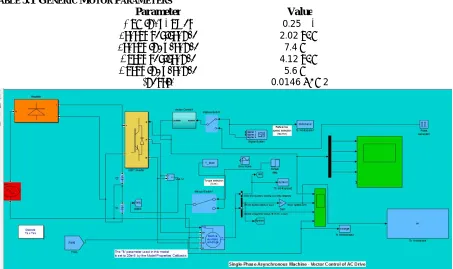
The overall system or simulation framework has been designed using MATLAB development platform and a 0.25HP AC servo motor has been used for simulating system model. The nominal motor parameters taken into consideration of system implementation are given as follows:

TABLE 5.1 GENERIC MOTOR PARAMETERS

Parameter Value

0.25

2.02 ℎ

7.4

4.12 ℎ

5.6

0.0146 2

Fig 8: Simulink Model for servo motor control

Fig 9 Nominal Speed Response for different loads

The speed of the system for various load conditions is shown in the Fig 9. The graphs clearly shows that the time required to meet the specified speed.

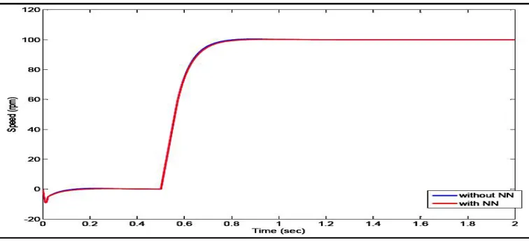
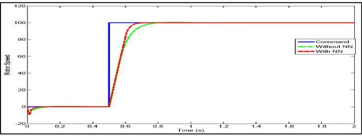
Fig 10 Comparison of response with and without neural network tuning (lesser parameter variations)

With the non-linear characteristics the response of the system varies with and without the software for tuning the controller to ensemble the same for the plant as shown in Fig 10.

When there is larger variation in the load to match up it the speed of the motor should be varied this is accomplished using the Neural network. The Fig 11 shows the importance of the Neural network.

Fig 12 Speed Response for BFGS quasi-Newton back propagation

The BFGS quasi-Newton back propagation is used during the training phase which helps on providing the operating point for motor speed. The Fig 12 shows that the neural network will smoothly change the speed of the motor.

Fig 13 Speed Response for Bayesian regulation back propagation

The Bayesian regulation back propagation which helps on providing the operating point for motor speed. The Fig 13 shows that the neural network will smoothly change the speed of the motor.

The cyclic order which helps on providing the operating point for motor speed. The Fig 14 shows that the neural network will smoothly change the speed of the motor.

Fig 15 Speed Response for Scaled conjugate gradient back propagation algorithm

The Scaled conjugate gradient back propagation which helps on providing the operating point for motor speed. The Fig 15 shows that the neural network will smoothly change the speed of the motor.

Fig 16 Speed responses for different NN algorithms

The Fig 16 shows the different neural network will smoothly change the speed of the motor.

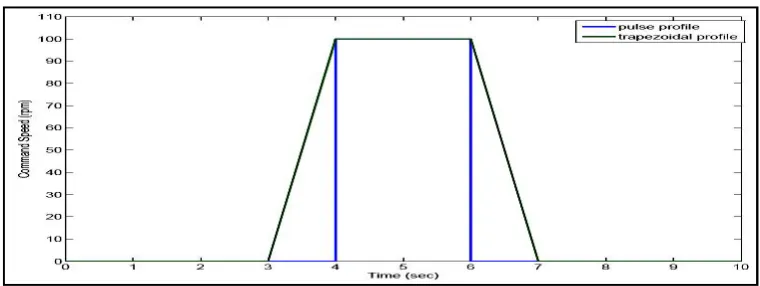
Fig 17 shows the command speed profiles for study of system during the presence of noise when the input pulse is trapezoidal or pulse one.

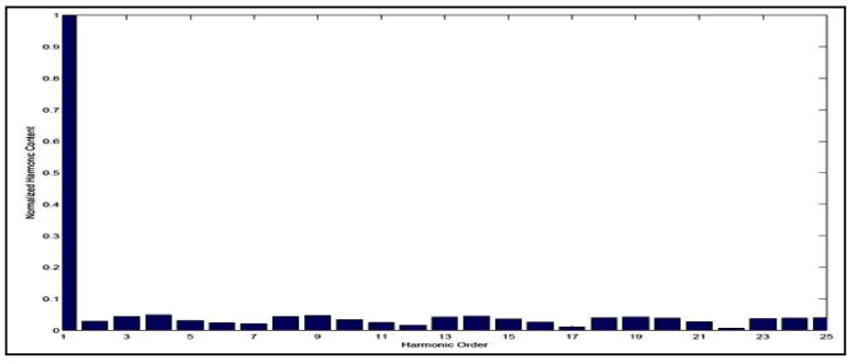
Fig 18 Harmonic content in command torque for rectangular pulse profile.

For the rectangular pulse as the input to the system the generated noise in the torque of the system is as shown in the Fig 18.

Fig 19 Harmonic content in motor speed for rectangular pulse profile

For the rectangular pulse as the input to the system the generated noise in the torque of the system is as shown in the Fig 19.

For the trapezoidal pulse as the input to the system the generated noise for the speed of the system is as shown in the Fig 20.

The harmonic content is higher for the rectangular speed profile as compared to the trapezoidal speed profile. The harmonic order is not affected by the neural algorithm.

The applicability of neural networks for servo control applications is demonstrated. Speed control of servo motor is presented with different training algorithms. The optimized artificial neural networks are suitable for the servo motor speed control.

VI. CONCLUSION

algorithms and their suitability for servo controls applications. Ultimately a Multi-layer Artificial Neural Networks (ANN) system has been designed and trained for modelling the plant parameter variations. Enhancements in the speed control performance have been presented for smaller variations and larger variations in the motor parameters and the load conditions. The speed control of servo motor has been analyzed using varied optimized artificial neural network based training schemes.

REFERENCES

[1] Kun Liu, Mulan Wang Jianmin Zuo,”Optimal PID Controller for Linear Servo-SystemUsing RBF Neural Networks”the Natural Science Fundamental Research Project for Universities of Jiangsu Province(08KJB460003),

[2] Fayez F. M. El-Sousy,”Intelligent Optimal Recurrent Wavelet Elman Neural Network Control System for Permanent-Magnet Synchronous Motor Servo Drive”,IEEE TRANSACTIONS ON INDUSTRIAL INFORMATICS, VOL. 9, NO. 4, NOVEMBER 2013

[3] Wang Panhai,”Hybrid Stepping Motor Position Servo System with On-line Trained Fuzzy Neural Network Controller”,0-7803-7474-61021S17.00 02002 IEEE

[4] Pyoung-Ho kim, Sa-Hyun sin, Hyung-Lae baek, Geum-Bae Cho, Speed control of AC servo motor neural networks. [5] S.N. Sivanandam , S.N. Deepa “Principles of soft computing”,

[6] Lalithamma G A, P S Puttaswamy and Kashyap D Dhruve. Article: Multi-layer Neural Network for Servo Motor Control. International Journal

of Computer Applications 71(14):32-37, June 2013. Published by Foundation of Computer Science, New York, USA

[7] K.J. Hunt, D. Sbarbaro, R. Zbikowski, P.J. Gawthrop, “Neural Networks for Control Systems: A Survey, Automatica”,pp. 1083-1122, 1992. [8] Hagan, Martin T., Howard B. Demuth, and Mark H. Beale. Neural Network design. Boston London: Pws Pub., 1996

[9] More J J, in Numerical Analysis, Lecture notes in Mathematics 630 (Springer Verlag, Germany) 1997, 105-116

[10] Ozgur Kisi, Erdal Uncuoglu, “Comparison of three back-propagation training algorithms for two case studies”, Indian Journal of Engineering & Materials Sciences, Vol 12 Oct 2005, pp 434-442.