Western University Western University
Scholarship@Western
Scholarship@Western
Electronic Thesis and Dissertation Repository
10-3-2013 12:00 AM
Computation Sequences for Series and Polynomials
Computation Sequences for Series and Polynomials
Yiming ZhangThe University of Western Ontario
Supervisor
Robert M. Corless
The University of Western Ontario
Graduate Program in Applied Mathematics
A thesis submitted in partial fulfillment of the requirements for the degree in Doctor of Philosophy
© Yiming Zhang 2013
Follow this and additional works at: https://ir.lib.uwo.ca/etd
Part of the Dynamic Systems Commons, Non-linear Dynamics Commons, Numerical Analysis and Computation Commons, and the Partial Differential Equations Commons
Recommended Citation Recommended Citation
Zhang, Yiming, "Computation Sequences for Series and Polynomials" (2013). Electronic Thesis and Dissertation Repository. 1683.
https://ir.lib.uwo.ca/etd/1683
Computation Sequences for Series and
Polynomials
(Thesis Format: Integrated-Article)
by
Yiming Zhang
Graduate Program in Applied Mathematics
A thesis submitted in partial fulfillment
of the requirements for the degree of
Doctor of Philosophy
The School of Graduate and Postdoctoral Studies
The University of Western Ontario
London, Ontario, Canada
Abstract
Approximation to the solutions of non-linear differential systems is very useful when the exact solutions are unattainable. Perturbation expansion replaces the system with a sequences of smaller problems, only the first of which is typically linear. This works well by hand for the first few terms, but higher order computations are typically too demanding for all but the most persistent. Symbolic computation is thus attractive; however, symbolic computation of the expansions almost always encounters intermediate expression swell, by which we mean exponential growth in subexpression size or repetitions. A successful management of spatial complexity is vital to compute meaningful results.
This thesis contains two parts. In the first part, we investigate a heat transfer problem where two-dimensional buoyancy-induced flow between two concentric cylinders is studied. Series expansion with respect to Rayleigh number is used to compute an approximation of a solution, using a symbolic-numeric algorithm. Computation sequences are used to help reduce the size of intermediate expressions. Up to 30th order solutions are computed. Accuracy,
validity and stability of the computed series solution are studied.
In the second part, Hilbert’s 16th problem is investigated to find the
Keywords: perturbation theory, large expression management, computa-tion sequences, heat transfer, free conveccomputa-tion, concentric cylinders, singular-ities, Quotient-Difference method, Hilbert’s 16th problem, limit cycles, focus
Co-Authorship Statement
Chapter 2 is co-authored with Rob Corless, and has been submitted for publi-cation. Rob Corless provided guidance through this work, and supervised the research. Rob Corless also reviewed and revised drafts of the paper.
Chapter 3 is co-authored with Rob Corless, Pei Yu, Marc Moreno Maza and Changbo Chen, which is accepted for publication. Rob Corless proposed the subject and supervised through out the whole period. He also reviewed the final draft of the paper. Pei Yu provided the guidance on Hilbert’s 16th
Acknowledgements
First of all, I would like to thank Rob Corless who guided me through this four wonderful years of my life and together we journey through the beautiful arts of applied mathematics. He has been helping me on every aspect of my research work. He shows great patience and trust, and he is always supportive and encouraging. It would not be possible for me to finish this thesis without his inspiration and constant help.
Within the department, I would like to thank Pei Yu for pouring his knowl-edge of dynamical system to me, and his willingness to help me whenever I meet problems. He devoted large amount of time on reviewing and rewriting almost every part of my draft work on the Hilbert 16th problem. There would be no such a paper without his contribution. I would like to thank Greg Reid for his very interesting super symmetry seminars. We had much fun marching to the field of super symmetry. I am thankful for David Jeffrey’s insightful discussions on the Painlev´e transcendents. Even though that work couldn’t ended as a paper, but I get a much deeper understanding of singularity struc-tures of PDEs. I also want to thank Chris Essex for sharing me his knowledge on teaching, who trusted me on taking his position to give lectures when he is occupied.
to thank Rong Xiao for his help on writing and compiling Mapleprocedures. Back at Brock, I want to thank Thomas Wolf who introduce me to the area of computer algebra. If it wasn’t for him, I would never had the opportunity to meet Rob and pursue my Ph.D. at Western.
Contents
Abstract ii
Co-Authorship Statement iv
Acknowledgements v
List of Tables viii
List of Figures ix
1 Introduction 1
1.1 Motivation . . . 1
1.2 Outline . . . 5
2 High-accuracy series solution for two-dimensional convection in a horizontal concentric cylinder∗ 10 2.1 Introduction . . . 10
2.2 Model Equations . . . 12
2.3 Solution by computation sequences: Perturbation in Rayleigh number . . . 14
2.3.1 Direct integration method . . . 16
2.3.2 The method of undetermined coefficients . . . 20
2.4 Cost of computation . . . 26
2.5 The accuracy of the series solution . . . 27
2.5.1 Stability of the solution . . . 35
2.6 Conclusions . . . 36
3 An application of regular chain theory to the study of limit
cycles† 40
3.1 Introduction . . . 40
3.2 Incremental solving . . . 44
3.3 The regular chains method . . . 46
3.3.1 Some definitions and examples for triangular decompo-sition . . . 47
3.3.2 Triangular decomposition algorithm . . . 50
3.3.3 A method based on modular techniques for computing triangular decomposition . . . 52
3.3.4 Isolating real roots of a regular chain . . . 56
3.4 Limit cycle and focus value . . . 57
3.5 Application to limit cycle computation . . . 59
3.5.1 Generic quadratic system . . . 60
3.5.2 A special cubic system . . . 64
3.6 Conclusion . . . 70
4 Concluding Remarks 76 A Proof of the shape of the general form . . . 79
B QD algorithm . . . 89
C Perturbation method and multiple time scale algorithm . . . . 92
D An example of focus value computation . . . 95
E Flaws in the paper of Lloyd and Pearson . . . 98
F Maple input for the quadratic example . . . 100
G Maple input for the cubic example . . . 101
Curriculum Vitae 106
†A version of this chapter has been accepted by the International Journal of Bifurcation
List of Tables
2.1 Table form ofT1
3, where, theK’s are coefficients of homogeneous
solution,C’s are coefficients of particular solution. For example,
K1 is the coefficient of K1r−1, where α =−1 and β = 0; C3 is
the coefficient of C3r−1ln(r), where α=−1 and β = 1. . . 22
2.2 Table form of R1
3. R’s are dummy variables representing the
coefficients of each term. For example, R2 is the coefficient of
R2r−5ln(r), where α=−5 and β = 1. . . 23
2.3 Accuracy analysis on the examples with nearby defects . . . . 31 2.4 Nearest pole locations of Rayleigh numberA, starting from the
origin. . . 32
A1 The non-zero component of theTm
k table. In side the boundary, the×represents some non-zero coefficientCTm
k ,α,β, while outside
the boundary all elements are zeros. . . 81 A2 The ∇2Tm
List of Figures
2.1 Sketch of the concentric cylinders . . . 13 2.2 Computation routine . . . 18 2.3 Left figure is the growth of number of terms in Tk and ψk
(O(k3)); the right one is the growth of number of entries in
the computation sequence for Tk and ψk (O(k6)). . . 27 2.4 Left figure is the log plot of residuals onTk and φk with R = 2
P = 0.02 k ≤ 30, the right one is the log of magnitude of Tk and φk with same parameter. . . 28 2.5 Residual ofT30. . . 29
2.6 The singularites and zeros of R = 2, P = 0.02 case (left), and
R= 2, P = 0.7 case (right) in the complex plane . . . 31 2.7 The stream contours ofR = 2, P = 0.7 case . . . 33 2.8 The stream contours ofR = 7/6, P = 0.2 case . . . 34 2.9 The ratios of k∆T,∆ψk
kRe(r,θ),Se(r,θ)k, whereA= 2000, R= 2 and P = 0.7 36
Chapter 1
Introduction
1.1
Motivation
The integration of multivariate non-linear differential systems is a very impor-tant but challenging subject in computer algebra. Exact solutions of many such systems, especially those with complicated nonlinear terms, are beyond the reach of today’s techniques. A popular workaround in computer algebra is to solve a nearby problem as an approximation with good accuracy. Perturba-tion theory is one such technique, which has a long history, and still remains popular [15, 23, 20, 22]. Other works on perturbation theory in practice in-clude [25, 24, 13, 16]. Due to their complicated structure, it is very natural to use computer algorithms to solve perturbation problems which usually involve the handling of large expressions. Thanks to the advances in both hardware and software techniques, we are able to compute perturbation expansions for systems that could not be solved before. In chapter 2, we use perturbation theory to solve the systems describing the two-dimensional heat convection of a fluid contained in two concentric cylinders. In chapter 3, we use pertur-bation theory to compute focus values which helps to identify the number of limit cycles on Hilbert’s 16th problem. In both applications, large expression
management techniques such as computation sequences and modular methods are the key technique.
ex-panded with respect to some parameter to form the series expansions. For example, to find the root of
x3+x−ε (1.1)
that goes to zero as ε→0.
We can expandx into Taylor series of ε, as follows:
x:=X k≥1
akεk (1.2)
By substitution, we obtain a sequence of equations for the ak,
a1−1 = 0
a2 = 0
a31+a3 = 0
3a21a2+a4 = 0
2a22a1+a1(2a1a3+a22) +a3a21+a5 = 0 · · ·
(1.3)
We solve these equations one after another and obtain the sequence of the coefficients {a1, a2, a3,· · · } as
{1, 0, −1, 0, 3, 0, −12, 0, 55, 0, −273, 0, 1428, 0, −7752, · · · }. (1.4) Therefore we arrive at the following approximation to the solution using the perturbation series:
can determine the radius of convergence directly. Here, the ak can be written as
ak:=
0 if k is even,
(−1)m
2m+1 3m
m
if k is odd, (1.6)
where m= (k−1)/2. Then the radius of convergence is lim k→∞ ak
ak+1
= limk→∞
s
a2k+1
a2k+3
= limm→∞
s
am
am+1 = lim m→∞ s 3m m
2m+ 1
2m+ 3
3m+3
m+1
= lim m→∞
s
(2m+ 3)(m+ 1)(2m+ 1)(2m+ 2) (2m+ 1)(3m+ 1)(3m+ 2)(3m+ 3) = 2/3√3
≈0.385.
(1.7)
If we setdε/dx to zero, which is 3x2+ 1 = 0, we obtainx=±i/√3. At these
points dx/dε = ∞, therefore ε = ∓i/3√3±i/√3 = ±2/3√3i, are the exact locations of the singularities, which match the radius of convergence. If we feed the series to Maple, it returns
∞
X
m=0
(−1)m 2m+ 1
3m
m
ε2m+1
=3εcosh 2 3arccosh( 3 2 √
3ε)
+2
√
3 9
−3− 81 4 ε
2sinh 2
3 arcsinh 3 2 √ 3ε q
1 + 274 ε2
,
translating of the perturbation expansion will quickly run out of memory. We consider the spatial complexity to be the number one issue to overcome.
parameter ε should be used in. To deal with this problem, singularity detec-tion techniques such as the Quotient-Difference (QD) algorithm (please see appendix B), are needed to ensure the validity of such solutions. In the previ-ous example, we input the series solution to the QD algorithm, the estimated nearest pole location is 0.395 which is within 3% of the true value.
1.2
Outline
In the first part of this thesis, we investigate the heat transfer of fluids con-tained in the annulus between two horizontally placed concentric cylinders. Two dimensional flow behavior for free convection∗ is studied. We used the
perturbation expansion with respect to Rayleigh numberA, following the work of Mack & Bishop [19] who computed series solution of the second order by hand. Corless et al. pushed the series solution to 10th order [7]. They
intro-duced computation sequences to simplify the intermediate expression swell. However at this order not many conclusions could be drawn firmly. We ex-tended the work of Corless et al. [7], optimized the computation sequences
and reprogrammed the symbolic-numerical solver, thereby pushing the result to 16th order. The solver applies a simplified direct integration method.
Dur-ing the computation of order kth solution, the algorithm computes particular
solutions according to each term of the inhomogeneous parts. The solutions are collected after all terms of the inhomogeneous parts are taken into con-sideration and then combined with the general solutions. At this point the coefficients in many terms of the solution are very complicated. We use new symbols to substitute these coefficients, and record the evaluation relation of these symbols in the computation sequences. These coefficients are not evalu-ated until the end of the symbolic stage when the desired order solutions are computed symbolically.
For a second, greatly improved algorithm, we recognized the pattern of solution of each order and summarized it into a general form. Applying the general form we designed a more efficient algorithm using the method of
known coefficients. This greatly reduces the size of intermediate expressions. The new algorithm decreased the spatial complexity from O(n7) to O(n4),
where the solution is truncated at nth order. We take advantage from this
efficiency and successfully computed solution to the 30th order. With this
high order solution, reliable information of the system can be extracted. As pointed out by Y.F Chang [8], 30th order solutions allow good estimates of
nearby singularities and their properties. Thereafter the series provides the range on Rayleigh number A, where within the range the solutions are valid. The QD method [14, 3, 9, 10, 1] is the main technique used here to detect singularities. Comparing to other methods, such as Pad´e approximants [3], the QD method has many advantages. It does not require information on the singularity structure a priori. It can handle the cases where defects† happen.
It works well with a small radius of convergence, where singularities are very close to the origin.
The errors of the computed series solutions are estimated using residual tests. The stability of the solution is also analyzed by perturbing the sys-tem with additional nonlinear terms. We observed the difference between the solutions and original ones compared to the size of the additional terms.
In the second part of the thesis, normal form theory and perturbation expansion are used to identify the number of limit cycles of quadratic and cubic planar polynomial systems. We investigated Hilbert’s 16th problem,
which asks for an upper bound of number on the limit cycles for a system in the form of
˙
x=F(x, y), y˙ =G(x, y), (1.9) whereF(x, y) andG(x, y) are degreek polynomials of variablesx andy, with real coefficients. The problem is narrowed to the case of small-amplitude limit cycles bifurcating from a center at the origin. In this case, the number of such limit cycles can be obtained by focus value computations. This problem has been solved for generic quadratic systems [4], where at most three such limit cycles could exist. For cubic systems, James and Lloyd obtained [18] a
†A defect in Pad´eapproximants is the case where a nearby singularity is accompanied
special cubic system with eight limit cycles. Yu and Corless [2009] showed the existence of nine limit cycles with the help of a numerical method for another special cubic system. We will symbolically compute the case of 9 limit cycles. In this work, the focus values are computed using perturbation theory on multiple time scales. The parameters of the system becomes the variable of the output focus values, which are multivariate polynomial equations. The real solutions of these equations will provide possible condition that the system consists certain number of limit cycles.
In order to find thenlimit cycles in a cubic system, there must be at leastn
Bibliography
[1] Allouche, H. and Cuyt, A. (2010). Reliable root detection with the QD-algorithm: When Bernoulli, Hadamard and Rutishauser cooperate. Applied numerical mathematics, 60(12):1188–1208.
[2] Aubry, P., Lazard, D., and Moreno Maza, M. (1999). On the theories of triangular sets. Journal of Symbolic Computation, 28(1-2):105–124.
[3] Baker, G. and Graves-Morris, P. (1996). Pad´e approximants, volume 59. Cambridge University Press.
[4] Bautin, N. (1952). On the number of limit cycles appearing with variation of the coefficients from an equilibrium state of the type of a focus or a center. Matematicheskii Sbornik, 72(1):181–196.
[5] Boyd, J. P. (2001). Chebyshev and Fourier spectral methods. Courier Dover Publications.
[6] Boyd, J. P. (2009). Large-degree asymptotics and exponential asymptotics for Fourier, Chebyshev and Hermite coefficients and Fourier transforms. Journal of Engineering Mathematics, 63(2-4):355–399.
[7] Corless, R. M., Jeffrey, D. J., Monagan, M. B., and Pratibha (1997). Two perturbation calculations in fluid mechanics using large-expression manage-ment. Journal of Symbolic Computation, 23(4):427–443.
[8] Corliss, G. and Chang, Y. (1982). Solving ordinary differential equations using taylor series. ACM Transactions on Mathematical Software (TOMS), 8(2):114–144.
[9] Cuyt, A. (1983). The QD-algorithm and multivariate Pad´e-approximants. Numerische Mathematik, 42(3):259–269.
[10] Cuyt, A. (1986). Multivariate Pad´e approximants revisited. BIT Numer-ical Mathematics, 26(1):71–79.
[11] Darboux, G. (1917). Principes de g´eom´etrie analytique. Paris.
[12] Deprit, A., Henrard, J., and Rom, A. (1970). Lunar ephemeris: Delau-nay’s theory revisited. Science, 168(3939):1569–1570.
[14] Henrici, P. (1974). Applied and Computational Complex Analysis: Vol.: 1.: Power Series, Integration, Conformal Mapping, Location of Zeros. Wiley New York.
[15] Hinch, E. (1991). Perturbation methods, volume 6. Cambridge University Press.
[16] Iooss, G. and Joseph, D. D. (1980). Elementary stability and bifurcation theory. Undergraduate Texts in Mathematics, New York: Springer, 1980, 1.
[17] Li, X., Moreno Maza, M., and Pan, W. (2009). Computations modulo regular chains. InProceedings of the 2009 international symposium on Sym-bolic and algebraic computation, pages 239–246. ACM.
[18] Lloyd, N. and Pearson, J. (2012). A cubic differential system with nine limit cycles. Journal of Applied Analysis and Computation, 2(3):293–304.
[19] Mack, L. and Bishop, E. (1968). Natural convection between horizontal concentric cylinders for low rayleigh numbers. The Quarterly Journal of Mechanics and Applied Mathematics, 21(2):223–241.
[20] Minorsky, N. (1991). Nonlinear Oscillations. Litton Educational Publish-ing, INC.
[21] Moreno Maza, M. (1999). On triangular decompositions of algebraic va-rieties. Technical report, TR 4/99, NAG Ltd, Oxford, UK.
[22] Nayfeh, A. H. and Mook, D. T. (2008). Nonlinear oscillations. Wiley. com.
[23] O’Malley, R. E. (1991). Singular perturbation methods for ordinary dif-ferential equations, volume 89. Springer-Verlag New York.
[24] Rand, R. H. and Armbruster, D. (1987). Perturbation methods, bifurca-tion theory and computer algebra, volume 65. Springer-Verlag New York.
Chapter 2
High-accuracy series solution for
two-dimensional convection in a
horizontal concentric cylinder
∗
2.1
Introduction
Heat transfer via natural convection in horizontal concentric cylinders has attracted much attention, due to its wide practical application and interest-ing dynamical behavior. Followinterest-ing the first comprehensive study by Liu, et al.(1961) [17] using air as the fluid, many experiments were conducted in the
1960’s by Bishop & Carley [5], Grigull & Hauf [12] and Lis [16] with different diameter ratio of cylinders and different Grashof number. Powe et al.[19, 20]
summarized their results on the convective flow of air and categorized the flow pattern into steady flow, oscillatory flow, three-dimensional spiral flow and multicellular flow. Labonia & Guj [15] conducted experiments using large Rayleigh numberA∈[0.9E5,3.3E5] and observed chaos (as one might expect nowadays).
In terms of computational studies, Mack and Bishop [18] applied a per-turbation expansion in the Rayleigh number A and obtained a series solution of second order. They suggested an approximation for a limiting value Alim above which their solution was not to be trusted; by implication, it was
sidered trustworthy forA < Alim. We will pursue this solution method to very high order in this present work, and give reliable accurate estimates forAlim. Custer & Shaughnessy [8] investigated very low Prandtl number P fluids using a double perturbation expansion in powers of the Grashof and Prandtl numbers. Kuehn & Goldstein [14] conducted both experimental and numerical (finite difference) studies for air and for water. Fant et al. [11] explored the
limiting case of zero Prandtl number using a so-called high Rayleigh number small gap asymptotic expansion. Yoo [21] gives a dual steady solution using a finite difference method. Desrayaud et al. reported a multi-cellular steady
state solution with small radius ratioR = 1.14 using a finite difference method [10] For a more comprehensive review please refer to [3].
Most numerical studies are conducted using finite difference methods. Each study chooses some specified settings of Prandtl number (type of the fluent), Rayleigh number (heat difference of the cylinders) and radius ratio (shape of the concentric cylinder). In the case of series solution, Mack & Bishop [18] gave a second order series solution valid for low Rayleigh number A. Further, their estimate of the upper limit of validity of their solution, which they called
Alim, was of unknown reliability. They used a perturbation expansion with respect to Rayleigh number to obtain the steady state solution of the stream and heat equations. Corlesset al. [7] investigated the problem in a computer
algebra point of view. In [7] the series solution of the problem was extended to 10th order by computer algebra using the then-novel technique of Large Expression Management. The principal concern of that work was efficient computer algebra.
In this article, we will extend that series solution to very high order in the Rayleigh number for arbitrary values of the parameters. The choice of parameters do influence the accuracy of the series solution, which will be discussed in section 5. We provide a reliable method for assessing precisely how small A must be for the solution to be valid.
generated from the double expansions. The pattern of the symbolic solution is recognized as some general form, and applied to develop a much more efficient algorithm using the method of unknown coefficients.
The current approach generates a symbolic program that, given values for Prandtl number P, and radius ratio R, can evaluate all terms up to O(A30)
exactly or in arbitrary high precision. Error analysis for the latter is discussed in section five as well. At this high order, reliable techniques for detecting and locating singularities become available. Here, we use the Quotient-Difference (QD) method to identify the structure of the singularities of the computed series solution, and thereafter provide an estimate on the validity of the serious solution.
2.2
Model Equations
Following the discussion of Mack and Bishop [18], the model contains two equations:
∇4ψ =A·L(T) + 1
P ·r
∂(∇2ψ, ψ)
∂(r, θ) , (2.1)
∇2T = 1
r
∂(T, ψ)
∂(r, θ) , (2.2)
where ψ is the stream function, T is temperature, P is the Prandtl number and A is the Rayleigh number, and
L(T) = sin(θ)∂T
∂r +
cos(θ)
r ∂T
∂θ , ∂(T, ψ)
∂(r, θ) =
∂T ∂r
∂ψ ∂θ −
∂T ∂θ
∂ψ ∂r ,
∇2 = ∂
2
∂r2 +
1
r ∂ ∂r +
1
r2
∂2
∂θ2, ∇ 4 =
∇2(∇2).
r′
o
r′
i
T′
i
T′
o
θ
Figure 2.1: Sketch of the concentric cylinders
quantities (all dimensional quantities are marked with primes).
r= r
′
r′
i
, r′ ∈[ri′, ro′], T = T
′ −T′
o
T′
i −To′
, T′ ∈[Ti′, To′], ψ = ψ
′
α′ ,
P = ν
′
α′ ,
A= gβ
′
ν′α′(T ′
i −To′)r3i .
(2.3)
Herer′
i is the radius of the inner cylinder,r0′ is the radius of the outer cylinder,
and their ratio is R = r′0
r′
i. We define r =
r′
r′
i, where r
′
i ≤ r′ ≤ r′o such that 1≤r≤R. T′
i and To′ represent the temperature of inner and outer boundary respectively. α′ = k′
ρ′C′
p is the fluid thermal diffusivity, k
′ is the thermal
con-ductivity, ρ′ is the density and C′
P is the specific heat capacity. ν′ is the fluid kinematic viscosity, g′ is the acceleration due to gravity andβ′ is coefficient of
The equation (2.1) and (2.2) obey the following boundary conditions:
T(1, θ) = 1, (2.4)
T(R, θ) = 0, (2.5)
ψ(1, θ) =ψ(R, θ) = ∂(ψ)
∂(r)(1, θ) =
∂(ψ)
∂(r)(R, θ) = 0, (2.6)
∂T
∂θ(r,0) =ψ(r,0) = ∂2ψ
∂θ2(r,0) = 0, (2.7)
∂T
∂θ(r, π) =ψ(r, π) = ∂2ψ
∂θ2(r, π) = 0. (2.8)
The boundary condition (2.4) and (2.5) define the temperatures of the annulus boundaries. The condition (2.6) ensures no flow passes through the boundaries. The initial conditions (2.7) and (2.8) define the flow to be symmetric with respect to the vertical line ofθ = 0 andθ =π.
2.3
Solution by computation sequences:
Per-turbation in Rayleigh number
Assume that T and ψ can be expanded in a convergent power series with respect to the Rayleigh number A,
T =
∞
X
j=0
AjTj(r, θ), (2.9)
ψ =
∞
X
j=1
Ajψj(r, θ). (2.10)
Substitute these power series in to equations (2.1) and (2.2), and isolate the coefficients of the same powers of A. This yields two infinite sets of equations,
∇2Tk = 1
r
k−1 X
j=0
∂(Tj, ψk−j)
∇4ψk= 1
P ·r
k−1 X
j=1
∂(∇2ψ
j, ψk−j)
∂(r, θ) +L(Tk−1), k = 1,2,3, . . . (2.12) According to the series expansion, the boundary conditions become
T0(1, θ) = 1, (2.13)
T0(R, θ) = 0, (2.14)
Tj(1, θ) =Tj(R, θ) = 0, j = 1,2,3, . . . , (2.15)
∂Tj
∂θ (r,0) = ∂Tj
∂θ (r, π) = 0, j = 0,1,2, . . . , (2.16) ψj(1, θ) =
∂ψj
∂r (1, θ) = ψj(R, θ) = ∂ψj
∂r (R, θ) = 0, j = 1,2,3, . . . , (2.17) ψj(r,0) =
∂2ψ
j
∂θ2 (r,0) =ψj(r, π) =
∂2ψ
j
∂θ2 (r, π) = 0, j = 1,2,3, . . . . (2.18)
We further expand ψk and Tk in Fourier series with respect to θ,
Tk(r, θ) = k
X
m=0
Tkm(r) cos(mθ), k= 0,1,2, . . . , (2.19)
ψk(r, θ) = k
X
m=0
ψkm(r) sin(mθ), k= 1,2,3, . . . , (2.20) to remove theθdependence. In the Fourier series, the odd numbered terms are zero if k is even, and even numbered terms are zero if k is odd. Substituting the Fourier series into equations (2.11) and (2.12) yields two infinite sequences of ordinary differential equations for functions Tm
k (r) and ψkm(r) which only depend on r. These new equations are of Euler type:
d2
dr2 +
1 r d dr − m2 r2
Tkm(r) =Rmk(r), (2.21)
d2
dr2 +
1 r d dr − m2 r2 d2
dr2 +
1 r d dr − m2 r2
where the inhomogeneous parts Rm
k(r) and Skm(r) are in terms of lower order
Tm
k (r) and ψkm(r), and always have the form
P
Cirαlnβ(r). Cii = 0,1,2· · · form a computation sequence, because each of them is defined in terms of previously computed Ck orKℓ, where k, ℓ < i. The general solutions of these Euler type equations are summations of homogeneous solutions and particular solutions. The homogeneous solutions are as follows,
TH,mk =
K1+K2ln(r) if m = 0,
K1r−m+K2rm if m 6= 0,
(2.23)
ψH,mk =
K1+K2ln(r) +K3r2+K4ln(r)r2 if m= 0,
K1/r+K2r+K3r3+K4ln(r)r if m= 1,
K1r−m+K2r−m+2+K3rm+K4rm+2 if m6= 0, m6= 1,
(2.24)
whereK1,K2,K3andK4 are unknown coefficients directly solvable the
bound-ary conditions. The particular solutions given the inhomogeneous parts in terms of Cα,βrα(ln(r))β are always computable. We use Maple to do the bookkeeping of the inhomogeneous terms and compute the particular solu-tions of the equasolu-tions (2.21) and (2.22). Observe that in (2.22) the operator (drd22 +
1
r d dr −
m2
r2 ) is applied twice, so a program that computes the particular
solution of (2.21) can be used to find the solution of (2.22) as well. In the fol-lowing section we will give an algorithm that computes the particular solution of (2.21).
2.3.1
Direct integration method
Equation (2.21) can be integrated using substitutions and an “integrating fac-tor”. For an inhomogeneous term in general form Crα(ln(r))β, we have
r2 d
2
dr2 +r
d dr −m
2
By linearity we may take C = 1 without loss of generality. We apply the substitution x= lnr to factorize the operator on T.
( d
2
dx2 −m
2)T = ( d
dx +m)( d
dx −m)T =e
αxxβ . (2.26) The equation is separated into two similar ones,
( d
dx +m)v =e
αxxβ , (2.27)
( d
dx −m)T =v , (2.28)
and (2.27) is integrated first (order does not matter since these operators commute†). The second substitution v = ueαx is introduced such that v′ =
(u′+αu)eαx and (2.27) becomes
du
dx + (α+m)u=x
β . (2.29)
Suppose α+m6= 0, (2.29) is integrated using the integration factor e(α+m)x,
u=e−(α+m)x
Z
xβe(α+m)xdx=e−(α+m)x
β
X
k=0
γke(α+m)xx(β−k)= β
X
k=0
γkx(β−k), (2.30) where γ0 = α+1m, γj = −γj−1α(β+−mj+1), j = 1,2, . . . , β. Thus, according to
v =ueαx and x= ln(r),
v =eαx
β
X
k=0
γkx(β−k) = β
X
k=0
γkrαln(r)(β−k),
γ0 =
1
α+m, γj =−
γj−1(β−j + 1)
α+m , j= 1,2, . . . , β .
(2.31)
†That is, we could equally well have chosen to integrate instead the pair (d
dx−m)u= eαxxβ followed by (d
T0
0 ψ11 ψ22 ψ31 ψ24 ψ15 ψ62
T1
1 T20 ψ33 ψ44 ψ35 ...
T2
2 T31 T40 ψ55 ...
T3
3 T42 T51
T4
4 T53
T5 5
k=0 k=1 k=2 k=3 k=4 k=5 k=6
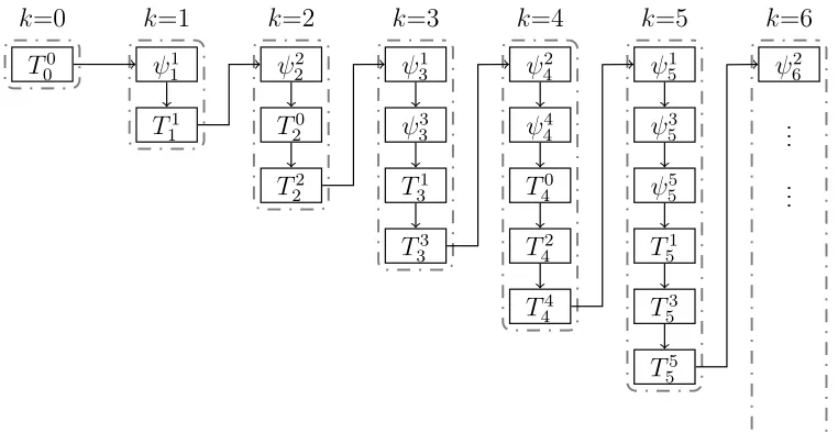
Figure 2.2: Computation routine
For the special caseα+m= 0, equation (2.29) degenerates intou′ =xβ which has the solution
u= 1
β+ 1x β+1,
v = 1
β+ 1x
β+1eαx = 1
β+ 1ln(r) β+1rα.
(2.32)
Observe that v is also in the form of PCrαlnβ(r), so (2.28) can be solved similarly to obtain T which is the particular solution of (2.21).
A Maple procedure has been written to systematically solve Tm
k and ψkm following a specific order of the equations (see Figure 2.2). The solution of
T0
0(r) is computed when the program starts. Then for each higher orderk >0,
ψm
k are computed first followed by Tkm, where m is increasing.
unknown coefficients.
The first several symbolic solutions generated by our program are printed here:
T00=K1+K2ln(r)
ψ11=
K3
r + 1/16K2r
3ln (r) +K
6rln (r)−1/32C1r3+K5r
T1
1 = −1/4
C4
r −1/2 K2K3
ln (r)r+ 1 128K
2
2r3ln (r) + 1/4C3ln (r)r+ 1/4K2K6r(ln (r))2
− 1
512C2r
3+K 8r
ψ22=K10−
1 128C16r
2
−92161 C17r4+
K9
r2 −
1
122881/PK2
2r6(ln (r))2
+ 1
147456C11r
6ln (r)
−35389441 C12r6+
1 128C15r
2ln (r)
−641 C9r2(ln (r))2+
1 2304C13r
4ln (r)
−3841 C7r4(ln (r))2
T20=
1 24576K2
3r6(ln (r))2
−2949121 C18r6ln (r) +
1
884736C19r
6+ 1
512K2
2K
6r4(ln (r))3
+ 1 2048C20r
4(ln (r))2
−40961 C21r4ln (r)−
1 16384C22r
4+ 1/16K
2K62r2(ln (r))3
+ 1 128C23r
2(ln (r))2
+ 1 512C24r
2ln (r)
−20481 C25r2+ 1/16C26(ln (r))2
−1/24K2K3K6(ln (r))3+ 1/8K2K3 2
ln (r) r2 + 1/8
C27
r2 +K13+K14ln (r)
T22= −1/32C37+K16r2−
1
331776C32r
4+ 1
64 C40
r2 −
1 384C33r
2(ln (r))3
− 1
768K2
2K
6r4(ln (r))3
+ 1/16C38ln (r)
r2 −
1 196608K2
3
1/Pr6(ln (r))2−1/16C36ln (r)−3/16K2K3K6(ln (r))2
+ 1
2359296C28r
6ln (r)
−566231041 C29r6− 1
1024C35r
2ln (r) + 1
512C34r
2(ln (r))2
−552961 C31r4ln (r)− 1
4608C30r
4(ln (r))2
· · · ·
The unknown constants K1, K2, . . .s are introduced when computing the
general solutions of the homogeneous equations, and they are efficiently com-putable from boundary conditions. The C′s are introduced during the
R, Prandtl number P and previously defined C′s and K′s. Maple does all
the bookkeeping of the evaluation information contained in computation se-quences of these unknown constants. Each time a symbolic solution of certain
Tm
k or ψkm is computed, the coefficients of the rαln(r)β terms are examined. Those coefficients that contain more than one monomial are substituted using a newC, and recorded in the appropriate computation sequence. In this way, the size of the input for the direct solving procedure are kept under control, which makes it possible to compute symbolic solutions to higher orders.
During the computation process, some K may share the same value as C, but we only keep their relationship and never substitute using theC, since the computational efficiency gained by doing so will be offset by more complicated bookkeeping.
This algorithm successfully computed solution to the 18th order, which
contains totally 111557 terms, 560 K′s, 83286 C′s, used about 22 hours and
41140.2MB memory.
2.3.2
The method of undetermined coefficients
With a careful investigation and verification we found the pattern of the sym-bolic solutions of each order, so that we can attack the expression swell in the intermediate steps. For k ≥1,Tm
k and ψmk obey the following general form‡
Tkm =
−m/2 X
α=−k/2
1+2Xα+k
β=0
CTm k ,2α,βr
2αlnβ
r+ m/2 X
α=−m/2+1
k−m/2+α+1 X
β=0
CTm k ,2α,βr
2αlnβ
r
+
3k/2−1 X
α=m/2+1
k+1 X
β=0
CTm k ,2α,βr
2αlnβr+ k
X
β=0
CTm k ,3k,βr
3klnβr ,
(2.33)
‡The uncommon half integers inαare used to summarize the even and odd case equations
ψkm =
−m/2−1 X
α=−k/2+1 2αX+k−1
β=0
Cψm k,2α,βr
2αlnβr+ m/2 X
α=−m/2
k−m/2+α
X
β=0
Cψm k,2α,βr
2αlnβr +
3k/2 X
α=m/2+1
k
X
β=0
Cψm k,2α,βr
2αlnβr .
(2.34) For a proof of this general form, please refer to Appendix A.
Using (2.33) and (2.34), we designed a new algorithm that starts from the known form of the symbolic solution and evaluates the coefficients according to that. Similar to the direct integration method, the coefficients are still distinguished, where the K’s are general solution coefficients, and the C’s are particular solution coefficients. This is not shown in the above general form, but is used in the algorithm to construct the Tm
k and ψkm. It is natural to distinguish K and C, since when the solutions are substituted to (2.21) and (2.22), the terms that contain K’s vanish and those contain C’s equal the inhomogeneous terms. Therefore, K’s are evaluated using the boundary conditions and C’s are computed using the unknown coefficient method.
In the new algorithm, solutions of Tkm, ψKm and their corresponding right hand sides Rm
k, Skm are stored in tables. The table structure helps to demon-strate how the terms containing C’s are mapped to the inhomogeneous parts. We also take advantage from less storage space and faster accessing time in-stead of using an explicit polynomial data structure. In the tables, the row index isα and column index isβ which are powers ofr and ln(r) respectively. The entries are the corresponding coefficients C or K. The procedure only needs to write down the coefficients of each entry other than the whole ex-pression containing rαln(r)β. To demonstrate the table structure, we take the
equation
d2
dr2 +
1
r d dr −
1
r2
rα\ln(r) β
β= 0 β = 1 β= 2 β= 3 β= 4
α=−3 C1 C2 0 0 0
α=−1 K1 C3 C4 C5 0
α= 1 K2 C6 C7 C8 C9
α= 3 C10 C11 C12 C13 C14
α= 5 C15 C16 C17 C18 C19
α= 7 C20 C21 C22 C23 C24
α= 9 C25 C26 C27 C28 0
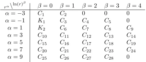
Table 2.1: Table form of T1
3, where, the K’s are coefficients of homogeneous
solution, C’s are coefficients of particular solution. For example,K1 is the
co-efficient ofK1r−1, whereα=−1 andβ = 0;C3is the coefficient ofC3r−1ln(r),
where α=−1 andβ = 1. as an example where
T1
3 =K1r−1+K2r+C1r−3+C2r−3ln2(r) +C3r−1ln(r) +C4r−1ln2(r) +C5r−1ln3(r)
+C6rln(r) +C7rln2(r) +C8rln3(r) +C9rln4(r) +C10r3+C11r3ln(r) +C12r3ln2(r)
+C13r3ln3(r) +C14r3ln4(r) +C15r5+C16r5ln(r) +C17r5ln2(r) +C18r5ln3(r)
+C19r5ln4(r) +C20r7+C21r7ln(r) +C22r7ln2(r) +C23r7ln3(r) +C24r7ln4(r)
+C25r9+C26r9ln(r) +C27r9ln2(r) +C28r9ln3(r),
(2.36)
and
R13=R1r−5+R2r−5ln(r) +R3r−3+R4r−3ln(r) +R5r−3ln2(r) +R6r−1+R7r−1ln(r)
+R8r−1ln2(r) +R9r−1ln3(r) +R10r+R11rln(r) +R12rln2(r) +R13rln3(r) +R14rln4(r)
+R15r3+R16r3ln(r) +R17r3ln2(r) +R18r3ln3(r) +R19r3ln4(r) +R20r5+R21r5ln(r)
+R22r5ln2(r) +R23r5ln3(r) +R24r5ln4(r) +R25r7+R26r7ln(r) +R27r7ln2(r)
+R28r7ln3(r),
(2.37)
are written in Table 2.1 and Table 2.2 respectively.
In order to compute the inhomogeneous coefficients C’s, the solution is substituted into (2.35). A term Crαln(r)β in Tm
rα\ln(r) β
β= 0 β = 1 β= 2 β= 3 β= 4
α=−5 R1 R2 0 0 0
α=−3 R3 R4 R5 0 0
α=−1 R6 R7 R8 R9 0
α= 1 R10 R11 R12 R13 R14
α= 3 R15 R16 R17 R18 R19
α= 5 R20 R21 R22 R23 R24
α= 7 R25 R26 R27 R28 0
Table 2.2: Table form of R1
3. R’s are dummy variables representing the
coef-ficients of each term. For example, R2 is the coefficient of R2r−5ln(r), where
α=−5 and β = 1. (d2
dr2 +
1
r d dr −
1
r2) operator into
d2
dr2 +
1 r d dr − 1 r2
(Crαln(r)β)
=C(α2−m2)rα−2ln(r)β + 2Cαβrα−2ln(r)β−1+Cβ(β−1)rα−2ln(r)β−2.
(2.38) Therefore, the elements in row α of the Table 2.1 will be mapped into row
α−2 of Table 2.2. This mapping can be written into a matrix form. For instance, we write the C’s in the fourth row (α = 3) of Table 2.1 as a vector
C=< C10, C11, C12, C13, C14 >T, and the fourth row (α= 1) of Table 2.2 into
a vectorR =< R10, R11, R12, R13, R14 >T. Then the mapping has the matrix
formM1C=R, where
M1 =
α2−m2 0 0 0 0
2αβ α2−m2 0 0 0
β(β−1) 2α(β+ 1) α2−m2 0 0
0 (β+ 1)(β) 2α(β+ 2) α2−m2 0
0 0 (β+ 2)(β+ 1) 2α(β+ 3) α2−m2 , (2.39)
α = 3, β = 1 and m = 1. This linear system can be generalized for any row of Tm
k and Rmk table. Suppose that there are j nonzero elements in row α of given Tm
α−2 row in Rm
k will have the same matrix form M1C=R, where
M1 =
α2−m2 0 0 0 0 0
2αβ α2 −m2 0 0 0 0
β(β−1) 2α(β+ 1) . .. 0 0 0
0 (β+ 1)(β) . .. ... 0 0
0 0 . .. ... α2−m2 0
0 0 0 . .. 2α(β+j−2) α2−m2 , (2.40)
and β is the powers of ln(r) of the first element in the α row ofTm k table. We can store the solutions of the linear system M1C = R for further
numerical evaluation. However, it is not efficient to do so. A better way that consumes less space is to store the matrixM1 and vectorR. When evaluating
C’s, the vectorR is substituted as numerical values. Similarly, (d2
dr2 +
1
r d dr −
1
r2)(
d2
dr2 +
1
r d dr −
1
r2) maps Cr
αln(r)β into
d2
dr2 +
1 r d dr − 1 r2 d2
dr2 +
1 r d dr − 1 r2
(Crαln(r)β) =(α2−m2)((α−2)2−m2)rα−4lnβr
+2(α2−m2)(α−2)β+ 2αβ((α−2)2−m2)rα−4lnβ−1r
+(α2−m2)β(β−1) + 4α(α−2)β(β−1) +β(β−1)((α−2)2−m2)rα−4lnβ−2r
+ (4α−2)β(β−1)(β−2)rα−4lnβ−3r+β(β
−1)(β−2)(β−3)rα−4lnβ−4r
(2.41) Therefore, the row α inψm
k table is mapped into α−4 row in the Skm table. A similar linear system can be constructed as M2C= S, where Cis the vector
consisting of j elements from row α inψm
Sm
k table. The matrix M2 has the following form,
M2 =
a1 0 0 0 0 0 0 0
b1 a2 0 0 0 0 0 0
c1 b2 a3 0 0 0 0 0
d1 c2 b3 . .. 0 0 0 0
e1 d2 c3 . .. ... 0 0 0
0 e2 d3 . .. ... ... 0 0
0 0 e3 . .. ... ... aj−1 0
0 0 0 . .. ... ... bj−1 aj
, (2.42) and
ai=(α2−m2)((α−2)2−m2),
bi=(α2−m2)2(α−2)(β+i−1) + 2α(β+i−1)((α−2)2−m2), ci=(α2−m2)(β+i−1)(β+i−2) + 4α(α−2)(β+i−1)(β+i−2)
+ (β+i−1)(β+i−2)((α−2)2−m2), di=(4α−2)(β+i−1)(β+i−2)(β+i−3), ei=(β+i−1)(β+i−2)(β+i−3)(β+i−4).
(2.43)
Here i = 1,2, . . . , j and β is the power of ln(r) in the first element in the α
row of ψm k table.
With the help of the table structure, evaluating the inhomogeneous coeffi-cients now turns into the process of solving a series of small linear system. We computed the condition number for all the matricesM’s up to 30thorder. The
average condition number is around 3.7 and maximum one is 10.4. Therefore, solving such linear systems numerically gives accurate solutions.
The new algorithm successfully computed series solution to the 30th order,
2.4
Cost of computation
Despite the space management techniques being used here, the size of the solutions and the corresponding computation sequences grow very fast. For example, in the direct integration method, T8 contains 715 terms with 67092
entries contained in the computation sequence for those terms;ψ8 contains 496
terms with 19796 entries in its corresponding computation sequence. Demon-strated in the left graph of Figure 2.3, the growth in number of terms isO(k3)§
In the right graph of Figure 2.3, the number of entries in the computation se-quence used in each order Tk and ψk have a growth rate of O(k6)¶. In fact, the construction of the coefficients in Tk and ψk involves O(k6) operations. Each operation using exact rational arithmetic has a cost that depends on the length of the integers involved, but for this problem the growth is modest and at 10th order the longest integers are about 100 digits long. Therefore a
solution truncated at order N, for example computing TN =PkN=0AkTk(r, θ) has spatial complexity O(13+ 23+· · ·+N6) = O(N7).
The difference between the size of kth order solutions and the number of
entries involved to compute them means the intermediate expressions during the kth order computation are much larger than the actual size of the same
order solution. In fact, there are many terms that share the same monomial of rαlnβ(r) in the intermediate expression. If these terms can be condensed without the loss of information, the solution process could be much improved. The new algorithm using unknown coefficients is motivated by this intention. In the new algorithm, solutions are constructed using the general form (2.33) and (2.34). The redundant computations in the first algorithm are eliminated since the coefficients C of the solutions have one to one mappings with the coefficients R in the corresponding right hand sides. Solving theC’s in the new algorithm does not involve the integration process which produces the redundant terms; instead it only requires the evaluation of several linear systems. For each Tm
k or ψkm there are 2k lower triangular matrices that need
§It can be directly computed from the general form.
Figure 2.3: Left figure is the growth of number of terms inTk and ψk (O(k3)); the right one is the growth of number of entries in the computation sequence for Tk and ψk (O(k6)).
to be solved, where the maximum size of the matrices isk×k. The spatial cost of computing Tm
k or ψmk is then O(2k×k2) which is O(k3). Then a solution truncated at orderN, has spatial complexity O(13+ 23+· · ·+N3) = O(N4).
Compared to the complexity of the direct integration method which isO(N7),
the new algorithm is seen to be much better.
2.5
The accuracy of the series solution
Both of the algorithms are based on the series expansion with respect to Rayleigh numberA, where
T =
∞
X
k=0
AkTk(r, θ), ψ =
∞
X
k=1
Akψk(r, θ).
Recall that in the above symbolic-numerical approaches, each Tk and φk are computed or written down symbolically in first step. These symbolic so-lutions are exact, since they strictly satisfy the equations (2.11), (2.12), and corresponding boundary conditions. The round off errors are introduced dur-ing the evaluation on the unknown coefficients K’s and C’s. Since higher order solutions dependent on lower order ones, the error accumulates during the evaluation process.
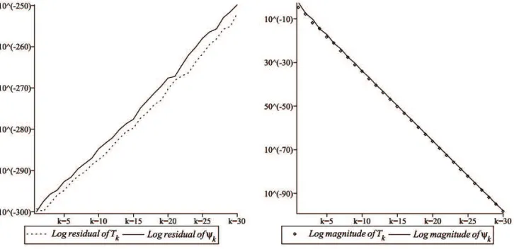
Figure 2.4: Left figure is the log plot of residuals on Tk and φk with R = 2
P = 0.02k≤30, the right one is the log of magnitude of Tk andφk with same parameter.
We use the residual of equation (2.11) and (2.12) where the numerical solutions are substituted in, to estimate the numerical error. For Nth order truncated solutionsTbN and ψbN, the residuals are defined as
εψk :=∇
4ψb
N −A·L(TbN)− 1
P ·r
∂(∇2ψb
N,ψbN)
∂(r, θ) ,
εTk :=∇
2Tb
N − 1
r
∂(TbN,ψbN)
∂(r, θ) .
(2.44)
In the left graph of Figure 2.4, thelog residual ofTkand φk are plotted for the
R= 2, P = 0.02 case. Note that the residuals are functions inr andθ, a local maximum of the residual is computed in the range of 1≤r≤R, 0≤θ ≤π. From Figure 2.4 we can see that the residuals are very small, and the errors are slowly adding up. In Figure 2.5, the residual ofT30 is computed withr ∈[1,2]
and θ ∈ [0, π]. The residual oscillates with in a bound when θ variates, but increases dramatically when r increase. However, the maximum size of the residual is very small.
Figure 2.5: Residual of T30.
convergence is determined by the nearest pole in the complex plane. Therefore, the pole locations of the series solution needs to be identified.
A possible way of obtaining the pole locations is by Pad´e approximants [4]. Pad´e approximants provides a rational function approximation based on the series expansion. The denominator of the approximation gives the information on pole locations. However, since the numbers of the poles and their structures are not known, it is hard to distinguish between the poles and noise. Pad´e approximants also faces severe difficulty when a defect happens where a pole is accompanied by a nearby zero [1]. Unfortunately, based on the results from the Pad´e approximants, the computed series solutions has many defects (as shown in Figure 2.6).
The QD method is used here to locate the nearby poles of the series ex-pansion with respect to the Rayleigh number A. The QD algorithm does not require any information on the poles a priori [13, 2, 9]. Unlike the Pad´e ap-proximants, it provides a mechanism that extracts pole location from the series inputk. Further more, the defect of nearby pole and zero have no significant
influence on QD method.
In order to demonstrate the performance of the QD algorithm on the defect, 10 input equations with a pole and a nearby zero are constructed as the input. The equations used to generate the series are as follows,
ex(x−0.999·10(−k))
x−1·10(−k) , k= 1,2, . . . ,10, (2.45)
wherekcontrols how close the defect is from the origin, and 1·10(−k)is the
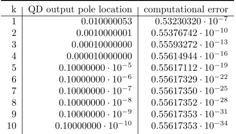
ex-act location of the pole. The distance between the defects and origin decreases by 10(−1) for each k. The noise ex is multiplied which doesn’t affect the na-ture of poles and zeros. Each of the equations in (2.45) is then expanded into Maclaurin series to the 10th order, which are the input of the QD algorithm. The computed pole locations and errors of the QD algorithm are presented in Table 2.3. Apparently, a defect near the expansion point has no impact on the ability of the QD algorithm to accurately locate the pole. In addition
k QD output pole location computational error 1 0.010000053 0.53230320·10−7
2 0.0010000001 0.55376742·10−10
3 0.00010000000 0.55593272·10−13
4 0.000010000000 0.55614944·10−16
5 0.10000000·10−5 0.55617112·10−19
6 0.10000000·10−6 0.55617329·10−22
7 0.10000000·10−7 0.55617350·10−25
8 0.10000000·10−8 0.55617352·10−28
9 0.10000000·10−9 0.55617353·10−31
10 0.10000000·10−10 0.55617353·10−34
Table 2.3: Accuracy analysis on the examples with nearby defects
the QD algorithm is very accurate even when the radius of convergence of the series expansion is almost zero. It has been shown [13] that the accuracy of the QD algorithm will only suffer when there are multiple poles in the same location or share the same moduli, for example: an essential singularity. In this case, the essential singularities can be mapped to nonessential singularities by logarithmic derivative.
Figure 2.6: The singularites and zeros of R = 2, P = 0.02 case (left), and
R= 2, P = 0.7 case (right) in the complex plane
2/(R−1) P = 0.02 P = 0.7 P = 7
2 125 2272 2880
3 441 5570 9433
4 1142 21193 39545
5 2460 69229 96243
6 4716 176510 196394
7 8367 239256 356767
8 14052 488791 597300 9 22599 904625 941098 10 34988 1163326 1414369 11 52315 1705722 2046395 12 75768 2418297 2869505
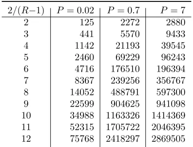
Table 2.4: Nearest pole locations of Rayleigh number A, starting from the origin.
can also use the equivalent conductivity, which is independent ofras the input. It has been shown by Mack & Bishop [18], the equivalent conductivity
keq = 1−A2
ln(R)∂T2
∂r |r=1
−A4
ln(R)∂T4
∂r |r=1
− · · · , (2.46) consists of the only terms that contributes to the overall heat transfer. The three different input series gives similar results as expected. We chose the series solution ofT as the input whereθandrare chosen randomly from the interval
θ ∈[0, π] andr∈[1, R]. The distance between the nearest pole and the origin is presented in Table 2.4, where Prandtl number is set to p = 0.02, p = 0.7 and p = 7 meaning mercury, air and water respectively. The corresponding radius ratio 2/(R−1) changes from 2 to 12. Comparing to the example of Mack & Bishop [18] where R = 2, P = 0.02, the QD algorithm returns 125 as the nearest conjugate pair of poles around the origin (A= 0). This is smaller than the 170 using only the second order series solution in Mack & Bishop’s estimation.
solutions within the radius. We now finally present some streamlines and isotherms that we believe to be highly accurate.
Figure 2.7: The stream contours of R = 2, P = 0.7 case
Figure 2.8: The stream contours of R = 7/6, P = 0.2 case
three clockwise rotating cells near the saddle points.
2.5.1
Stability of the solution
A more important (and traditional) question: is the computed solution stable? If we perturb equation (2.1) into,
∇4ψ =AL(T) + 1
P ·r
∂(∇2ψ, ψ)
∂(r, θ) +εf(r, θ), (2.47) and T =Te0+εTe1,ψ =ψe0+εψe1, thenTe1 and ψe1 can be computed by solving
the following new system,
∇4ψe1 =A
∂L ∂T(Te0)
+ 1
P ·r
"
∂(∇2ψe 0,ψe1)
∂(r, θ) +
∂(∇2ψe 1,ψe0)
∂(r, θ) #
+εf(r, θ), (2.48)
∇2Te1 =
1
r
"
∂(Te0,ψe1)
∂(r, θ) +
∂(Te1,ψe0)
∂(r, θ) #
, (2.49)
This system is more complicated than the original system. A faster way is to change the basic solution T0
0 to T00 +εf symbolically, for example f =
(r−1)(R−r)rαln(r)β such that it still obeys the boundary conditions. Then we generate the solutions as T =T0+ε∆T and ψ =ψ0+ε∆ψ. We substitute
these solutions back to the original system and compute the residual containing
ε
εRe(r, θ) =∇4ψ−AL(T)− 1
P ·r
∂(∇2ψ, ψ)
∂(r, θ) , (2.50)
εSe(r, θ) =∇2T − 1 r
∂(T, ψ)
∂(r, θ) , (2.51)
The solution is stable if k∆T,∆ψk ≈ kRe(r, θ),Se(r, θ)k. It is ill-conditioned if
k∆T,∆ψk ≫ kRe(r, θ),Se(r, θ)k. In the case of A= 2000, R = 2 and P = 0.7, the maximum ratio of k∆T,∆ψk
kRe(r,θ),Se(r,θ)k is around 0.07, which means the solution is
Figure 2.9: The ratios of k∆T,∆ψk
kRe(r,θ),Se(r,θ)k, whereA= 2000, R= 2 and P = 0.7
2.6
Conclusions
Computation sequences and the discovery of a general form expression im-prove the algorithm so that we can compute very high order series solutions. Obviously the method used here is slower than numerical methods. Still, with such solutions, much more information can be extracted, such as the singu-larity structures, and therefore the radius of convergence. The accuracy and stability of the series solutions are also verified.
the algorithm takes many steps to go around a pole on the real axis especially when there are nearby poles on the complex plane. Moreover, we lose the economical general form expression, which is valid only near A = 0. On the plus side, one can still guarantee accuracy using analytic continuation by using small steps and computing the residual. If the overall errors can be controlled then much more interesting results could be discovered, such as going around poles using different paths, and a better understanding of the solution. This will be examined in future work.
Within the radius of convergence, the series solution computed here offers a useful reference for the existing results computed from pure numerical methods such as the finite difference method. Due to its high accuracy many details of the flows can be obtained. The high order solution give us the chance to observe the singularity structures more clearly, which could be used as an “map” for future work. Algorithms such as analytic continuation will certainly benefit from this.
Finally, the spatial management techniques, especially computation se-quences can be applied to other similar problems which use perturbation series to describe the solutions. At the most simple, the same problem with different boundary conditions. We have only investigated the simplest of these. For flow in porous media, other boundary conditions are of interest. We remark that the technique of computation sequences is by no means restricted to this PDE, however.
Bibliography
[1] Abd-Elall, L., Delves, L., and Reid, J. (1970). A numerical method for locating the zeros and poles of a meromorphic function. Numerical methods for nonlinear algebraic equations, pages 47–59.
[2] Allouche, H. and Cuyt, A. (2010). Reliable root detection with the QD-algorithm: When Bernoulli, Hadamard and Rutishauser cooperate. Applied numerical mathematics, 60(12):1188–1208.
review of buoyancy-induced flow transitions in horizontal annuli. Interna-tional Journal of Thermal Sciences, 49(12):2231–2241.
[4] Baker, G. and Graves-Morris, P. (1996). Pad´e approximants, volume 59. Cambridge University Press.
[5] Bishop, E. and Carley, C. (1966). Photographic studies of natural convec-tion between concentric cylinders. InProc. Heat Transfer Fluid Mech. Inst, volume 6, pages 63–78.
[6] Boyd, J. P. (2001). Chebyshev and Fourier spectral methods. Courier Dover Publications.
[7] Corless, R. M., Jeffrey, D. J., Monagan, M. B., and Pratibha (1997). Two perturbation calculations in fluid mechanics using large-expression manage-ment. Journal of Symbolic Computation, 23(4):427–443.
[8] Custer, J. and Shaughnessy, E. (1977). Thermoconvective motion of low Prandtl number fluids within a horizontal cylindrical annulus. Journal of Heat Transfer, 99:596.
[9] Cuyt, A. (2008). Handbook of continued fractions for special functions. Springer.
[10] Desrayaud, G., Lauriat, G., and Cadiou, P. (2000). Thermoconvective instabilities in a narrow horizontal air-filled annulus. International journal of heat and fluid flow, 21(1):65–73.
[11] Fant, D., Prusa, J., and Rothmayer, A. (1988). Unsteady multicellular natural convection in a narrow horizontal cylindrical annulus. In AIAA, ASME, SIAM, and APS, National Fluid Dynamics Congress, volume 1, pages 1922–1934.
[12] Grigull, U. and Hauf, W. (1966). Natural convection in horizontal cylin-drical annuli (tests for measuring heat-transfer coefficients in horizontal annulus filled with gas and visualization of flow). In International Heat Transfer Conference, 3 RD, CHICAGO, ILL, pages 182–195.
[14] Kuehn, T. and Goldstein, R. (1976). An experimental and theoretical study of natural convection in the annulus between horizontal concentric cylinders. Journal of Fluid Mechanics, 74(04):695–719.
[15] Labonia, G. and Guj, G. (1998). Natural convection in a horizontal con-centric cylindrical annulus: oscillatory flow and transition to chaos. Journal of Fluid Mechanics, 375:179–202.
[16] Lis, J. (1966). Experimental investigation of natural convection heat transfer in simple and obstructed horizontal annuli. In Proceeding of the 3rd International Heat Transfer Conference, volume 2, pages 196–204.
[17] Liu, C., Mueller, W., and Landis, F. (1961). Natural convection heat transfer in long horizontal cylindrical annuli. International Developments in Heat Transfer, (117):976–984.
[18] Mack, L. and Bishop, E. (1968). Natural convection between horizontal concentric cylinders for low rayleigh numbers. The Quarterly Journal of Mechanics and Applied Mathematics, 21(2):223–241.
[19] Powe, R., Carley, C., and Bishop, E. (1969). Free convective flow patterns in cylindrical annuli. Journal of Heat Transfer, 91:310.
[20] Powe, R., Carley, C., and Carruth, S. (1971). A numerical solution for natural convection in cylindrical annuli. Journal of Heat Transfer, 93:210.
Chapter 3
An application of regular chain
theory to the study of limit
cycles
∗
3.1
Introduction
In the field of dynamical systems, an interesting topic is the study of the number of limit cycles of a given system. For example, Hilbert’s 16th problem asks for an upper bound of the number of limit cycles for the system
˙
x=F(x, y), y˙ =G(x, y), (3.1) whereF(x, y) andG(x, y) are degreek polynomials of variablesx andy, with real coefficients. No results are established for generic cubic systems.
In the case of finding small-amplitude limit cycles bifurcating from an ele-mentary center or a focus point based on focus value computation, the problem has been completely solved only for generic quadratic systems [3], which can have three limit cycles in the vicinity of such a singular point. For cubic systems, James and Llyod obtained [25] a formal construction, via symbolic computation, of a special cubic system with eight limit cycles. In [52], Yu and Corless showed the existence of nine limit cycles with the help of a numerical
∗A version of this chapter has been accepted by the International Journal of Bifurcation
method for another special cubic system.
Very recently, Lloyd and Pearson [32] claimed to be the first to obtain a formal construction, via symbolic computation, of a new cubic system with nine limit cycles. A key step of their derivation is to show that two bivariate polynomials R1 and R2 have real solutions. They found that the resultant of
R1 andR2 had a real solution and then concluded thatR1 and R2 would have
a real common solution. This is not always true. In fact, the existence of a real solution of the resultant of two bivariate polynomials does not necessarily imply the existence of a common real solution for the original two polynomial equations. For example, given R1 = y2 +x+ 1 and R2 = y2 + 2x+ 1 with
x < y, the resultant of R1 and R2 in y is x2, which has a real solution x= 0.
However the two equations R1 = R2 = 0 actually do not have common real
solutions. In addition, a similar flawed conclusion was made by the authors when they were claiming that the existence of real solutions for R1 =R2 = 0
was implying the existence of real solutions for a trivariate polynomial systems Ψ1 = Ψ2 = Ψ3 = 0. Therefore, the proof given by Lloyd and Pearson in [32]
is not complete. (For a more complete explanation, please refer to Appendix E.)
In the present paper, we formally prove that a specific cubic dynamical system has nine limit cycles. Our strategy is as follows. Given a cubic dy-namical system, we reduce the fact that this system has (at least) nine limit cycles to testing whether a given semi-algebraic set is empty or not. This test is based on a symbolic procedure capable of producing an exact representation for each real solution of any system of polynomial equations and inequalities. Once one such real solution has been found, then this procedure can be halted and non-emptiness has been formally established. Therefore, our approach does not have the flaws of [32].
The symbolic computation of small limit cycles involves finding the com-mon roots of a non-linear polynomial system consisting of n focus values