Behaviors and Characteristics Study of the Electron Beam for
Lens System in a Scanning Electron Microscope
Mohammed A. Hussein Mohanad Q. Kareem, University of Kirkuk University of Kirkuk College of agriculture / Hawija College of Science Dept. of mechanization and agricultural equipment Dept. of physics
[email protected] [email protected]
Abstract
This work aims to study the behaviors and characteristics of the electron beam within the optical column in a thermionic scanning electron microscope (SEM) and the focusing capability using a numerical computation and an optics-based calculation. The beam spot size is estimated by theoretical calculation. Investigate the SEM performance for various design parameters through a numerical analysis and an optics-based calculation, a combination of two approaches gives more detailed information than a single approach in investigating an extremely small beam spot by demagni cation through the magnetic lens system in a SEM column. Keywords: Magnetic lens; Scanning electron microscopy; Thermionic emission; Numerical analysis; Beam trajectory.
1. Introduction
Represents a scanning electron microscope (SEM) is one the most
share due to its effectiveness over the cost. An actual resolution of SEM is 50 times larger than the theoretical limit because of irregular electron gun size, aberration, energy spread, etc. Therefore, new generation of SEMs is focused on improvement an electron beam source to give high brightness and low energy spread, and an electron lens system with less aberration.
To enhance the resolution of SEM Compared with the optical microscope, we use accelerated electrons of extremely short wavelength less than 0.01nm. While optical microscope use a visible light source in the range of 300– 700nm wavelength, a SEM uses The electrons being accelerated by high voltage applied on the lament, , and being focused on the specimen surface by electro-magnetic lenses [5]. The SEM are similar to an optical microscope in the structure and principle. For focusing light rays in the optical microscope use us the Optical lenses instead of electromagnetic lenses in a SEM. Fundamental difference appear in a SEM. The electromagnetic lens consist of an electric coil pass through it the current, generates magnetic ux within a concentrated small volume by [6]. We can decrease the wavelength of an
electron beam by increasing the acceleration voltage applied on the emitted beam source, which is useful to the image resolution. There are many parameters constrains the enhancement of SEM resolution. Design a poor beam source as well as an improper lenses arrangement.
numerical analysis uses widely to facilitate the design of the electron lenses therefore munro used a finite element method from first order to analyze electron lenses.[7] By the Lorentz force The magnetic ux associated with acceleration voltage makes the electron beam travel along optical column and be focused at a focal point. The is by there are various factors effect on the focusing such as an electric current applied on the coil, geometry and arrangement of the lenses in the optical column, and acceleration voltage.
subsequent lenses should be controlled within of nanometer. The other, chromatic aberration should be decreased, by placing a specially designed stigmator and the electron beams emitted from a lament must be suf ciently stabilized.
In this work, we focus on the design of the lens system by employing a numerical analysis and geometrical optics for the SEM. Through these analyses, beam focusing characteristics and the resulting lens aberrations can be estimated. The beam trajectory analysis under various selections of the lenses by simulating the SEM system using an Munro software [7], providing a guideline in designing an ef cient SEM.
2. Numerical analysis of the electron optical system
The schematic diagram of
thermionic SEM, as shown in Fig. 1 illustrate consist of an optical column, devices to improve the beam focusing characteristics, and a detector collecting secondary electrons emitted from the specimen. Electromagnetic lens to focus the electron beam spot. If the lens system is not appropriately designed or misaligned, the shape of abeam spot will be a bad shape or blurry. Therefore, a precise analysis of the beam focus is required to ensure a high-performance SEM in terms of small beam spot size and less aberration. we consider two methods: a numerical analysis using abeam tracing program M21and a calculation based on a geometric optics. Therefore, a combination of the calculation and the numerical analysis gives a strong basis for an optimal design of the lens system in a SEM.
3. Background of the numerical analysis
Using M21 software from numerical analysis we performed An electron beam trajectory under the magnetic fields on three lenses. Firstly, analyze of distribution of the electromagnetic eld for the designed lenses each magnetic flux is distributed around the lens and the magnitude is enough to deflect the electron beams. As the electron beams pass through three electromagnetic lenses, the nal beam spot is formed after demagnification through the subsequent lenses, of which diameter is determined by the ratio of the focal lengths to the displacements among lenses.
Here, we introduce a principle of the electron beam tracing by using the governing equations. The equations describing the electromagnetic field generated by the magnetic enses are given by the Maxwell’s equations as follows:
∇ ∗ 𝐸 = −𝜕𝐵
𝜕𝑡 (1)
∇ ∗ 𝐻 = 𝐽 (2)
∇. 𝐷 = 𝜌 (3)
∇. 𝐵 = 0 (4)
Where E is the electric eld intensity, B is the magnetic ux density, D is the electric ux density, H is the magnetic eld intensity, J is the current density, and r is the electrical resistivity. If we set the magnetic vector potential A given by Eq. (5), the distribution of A can be expressed as Eq. (6), by uniting Maxwell’s equations: 𝐵 = ∇ ∗ 𝐴 (5)
1 𝜇𝛻 ∗ ∇ ∗ 𝐴 − 𝜌 𝜕𝐴 𝜕𝑡 = 0 (6)
Where m is the permeability of the material. The distribution of A is then calculated by minimizing the vibrational functional [9]: 𝐹 = ∫ 𝜔[1 𝜇(∇ ∗ 𝐴). (∇ ∗ 𝐴) − 𝐽. 𝐴]𝑑𝜔 = 0 (7)
Based on the calculated magnetic elds, the electron beam tracing under the formed magnetic elds on each lens is performed by solving the paraxial ray Eq. (7): 𝑟∥ (𝑧) + 𝑒 8𝑚𝑣𝐵 2(𝑧)𝑟(𝑧) = 0 (8)
where e/m is the charge/mass ratio of the electron and V is the beam voltage .
4. Magnetic lens system
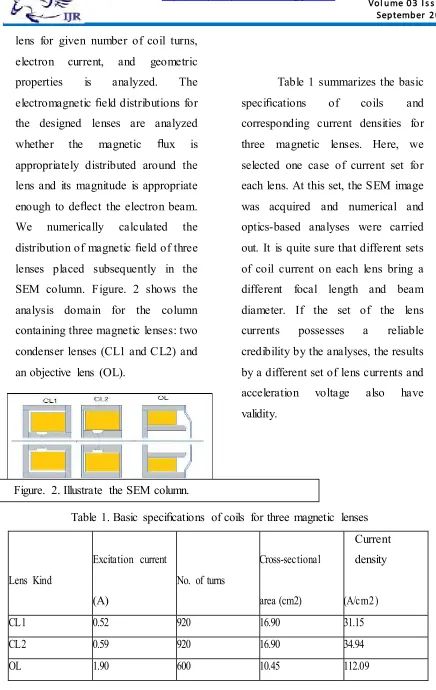
lens for given number of coil turns, electron current, and geometric properties is analyzed. The electromagnetic eld distributions for the designed lenses are analyzed whether the magnetic ux is appropriately distributed around the lens and its magnitude is appropriate enough to de ect the electron beam. We numerically calculated the distribution of magnetic eld of three lenses placed subsequently in the SEM column. Figure. 2 shows the analysis domain for the column containing three magnetic lenses: two condenser lenses (CL1 and CL2) and an objective lens (OL).
Table 1 summarizes the basic speci cations of coils and corresponding current densities for three magnetic lenses. Here, we selected one case of current set for each lens. At this set, the SEM image was acquired and numerical and optics-based analyses were carried out. It is quite sure that different sets of coil current on each lens bring a different focal length and beam diameter. If the set of the lens currents possesses a reliable credibility by the analyses, the results by a different set of lens currents and acceleration voltage also have validity.
Table 1. Basic speci cations of coils for three magnetic lenses
Lens Kind
Excitation current
No. of turns
Cross-sectional
Current density
(A) area (cm2) (A/cm2)
CL1 0.52 920 16.90 31.15
CL2 0.59 920 16.90 34.94
OL 1.90 600 10.45 112.09
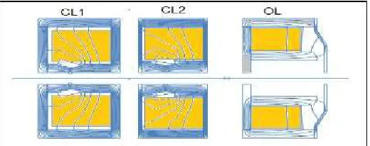
Figure. 3 illustrates the distribution of magnetic ux in the column, showing that the magnetic elds are concentrated around the pole piece regions of the three magnetic lenses. Figure. 4 represent the variation of the axial component of magnetic ux (Bz) along the axial distance from the electron gun. It is found that the magnetic ux shows peak at the narrow-spaced pole-piece locations. Detailed results of three peak values are compared in Table 2. It is noted that the amount of the peak ux of the OL is smaller than those of two condenser lenses because the
OL has a larger gap of pole piece in order to install magnetic de ectors inside the lens. Even if coil currents on CL1 and CL2 are closely imposed, the corresponding magnetic uxes on both lenses show a large difference. This implies that the magnetic ux on CL2 is affected by magnetic ux on CL1 because the length to the pole piece of CL2 from the end line of CL1 is shorter than that of CL1 from the start line of CL1. These analysis results are then connected to the ray tracing analysis to predict the beam trajectory.
Figure 3. Distribution of the magnetic potential in the column.
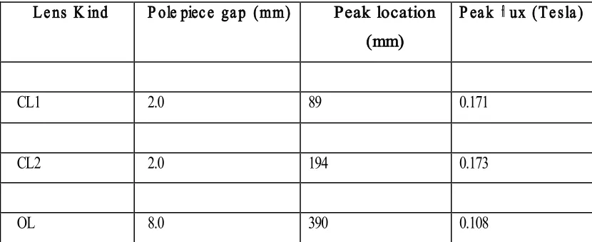
Table 2. Summary of electromagnetic analysis of magnetic lenses
Le ns K ind P ole piec e ga p (mm) Peak location (mm)
P ea k ux (Te sla )
CL1 2.0 89 0.171
CL2 2.0 194 0.173
OL 8.0 390 0.108
5. Electron beam trajectory
A ray tracing of electron beams is then performed by taking into account the calculated magnetic eld. Fig. 5 represents the estimated beam trajectory by solving the ray tracing equation, showing that three crossovers are formed by three magnetic lenses.
Table 3 summarizes the beam tracing results for the three lenses. The focal lengths are obtained by calculating the distances from the refracting position to the crossing position at each lens. Comparison of these results will be discussed in the next section.
Table 3 summarizes the beam tracing results for the three lenses
Lens Kind Beam refraction position Zp(mm)
Position of plane image Zi(mm)
Focal length F(mm)
CL1 89.33 93.975 4.42
CL2 194.33 198.937 4.40
OL 361.92 372.950 10.34
As the electron beam is focused by the subsequent lenses arrangement and acceleration
secondary electrons from the specimen. The secondary electrons are dedicated to the SEM image, which is determined by the amount of secondary electrons emitted from the surface of the specimen.
The amount of secondary electrons increases as the beam spot size is
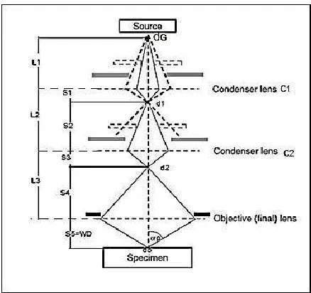
small as possible to have strong current density. Thus, the beam spot size and uniform beam shape are crucial to obtain a high focused image. The beam spot size is approximately computed by employing a geometric optics which explains the demagni cation process formed by lenses (Fig. 6).
R(mm)
Z(mm)
Figure. 5. Ray tracing results from the beam source to the image plane.
Figure. 6. Schematic diagram for focusing lenses.
The numerical analysis by commercial program, demonstrated in
all necessary information on beam characteristics. The beam intensity and the brightness are some of the characteristics not provided by numerical analysis. A calculation by geometric optics on the lens system supplements this weakness.
So far, we assumed that each magnetic ux Bz(z) of the three lenses shows a symmetric shape, which makes the computation of the focal length simple as Eq. (11). However, even if the ux distributions of other two lenses keep almost symmetric bell shapes, the magnetic ux of the object lens is bell shaped but not symmetric: the left side of the shape is gentler than the right side. It limits the direct use of Eq. (10), hence a more precise calculation of magnetic ux is required. Here we adopt a numerical integration to obtain the focal lengths from the magnetic ux for three lenses, which is shown in eq. (10) .The results of focal lengths for each lens by numerical integration are shown in Table 4. We can see slightly different results compared with the results obtained by simple bell-shaped assumption on the magnetic ux. For a simple calculation, the focal length
computation based on the bell-shaped magnetic ux is still acceptable.
The axial magnetic ux is determined through a numerical analysis as introduced in the previous section. This implies that a different set of coil currents or pole piece shapes generates different magnetic ux, yielding a different focal length in the lens. Since the SEM consists of three lenses focusing the electron beam consecutively, the total demagni cation of a three-lens system yields a nal focused spot d0:
𝑑𝑜 =𝑓1 𝑓2 𝑓3
𝑝1 𝑝2 𝑝3𝑑𝑐 (9)
1
𝑓=
𝑒
8𝑚𝑉∫ 𝐵𝑧
2 +∞
−∞
𝑑𝑧 (10)
𝑓 = 2𝑎
𝜋𝑘2 𝑓𝑜𝑟 𝑘
2 ≪ 1 (11)
𝑑𝑜 = (4𝐼𝑃 𝜋2𝛽)
1 2𝛼𝑝−1
(12)
of 50 V and the virtually focused beam diameter are estimated. According to the analysis, the beam diameter at the cathode after being focused by the biased voltage and acceleration voltage of 20 kV turns out to be around 33 mm.
Viewing Eq. (9), it is noted that once all focal lengths and displacements are determined the nal probe diameter can be determined and the demagni cation through three lenses is also computed.
Table 4. Comparison of the focal lengths Lens Kind Analytical solution
(mm)
Analytical with numerical integral (mm)
CL1 5.11 7.65
CL2 6.45 7.62
OL 14.65 15.67
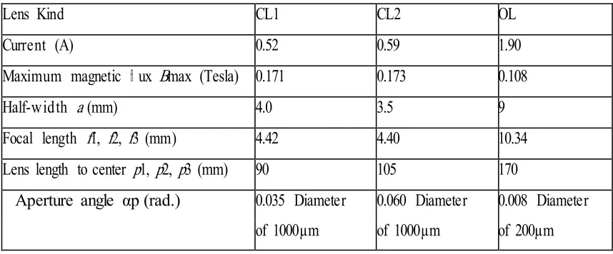
The probe diameter is estimated by employing Eq. (9) with the help of formed by the focal lengths computed from Eq. (10).
Table 5. Computation of focal lengths, aperture angles, and estimated probe diameter for given coil currents and acceleration voltage of 20 kV.
Lens Kind CL1 CL2 OL
Current (A) 0.52 0.59 1.90
Maximum magnetic ux Bmax (Tesla) 0.171 0.173 0.108
Half-width a (mm) 4.0 3.5 9
Focal length f1, f2, f3 (mm) 4.42 4.40 10.34
Lens length to center p1, p2, p3 (mm) 90 105 170
Aperture angle αp (rad.) 0.035 Diameter 0.060 Diameter 0.008 Diameter of 1000µm of 1000µm of 200µm
beam tracing and focusing in a lens system contributes to an optimal design of the lens system in an SEM before manufacture. This analysis necessary To secure a highly demagni ed beam spot. the focal lengths formed by the magnetic ux on magnetic lenses, which are generated by the coil current and the shape of pole piece, were investigated. To obtain a minimized probe beam spot, the demagni cation ratio on each lens should be as large as possible unless the lenses have undesirable aberrations. Employed both numerical analysis program and optics calculation to analyze the focal length. Two ways were reciprocal in terms of being able to extract complementary parameters and they showed a quite satisfactory agreement. When two ways are integrated, rather than a single way, in the early stage of lens system design can be easily obtained for the desired focal length and other parameters. From the a numerical analysis and geometric optics, The probe diameter, which is an important factor in SEM performance, can be estimated. The
validity of the numerical analysis and optics-based computation for the lens system is proved by measuring the probe diameter that results in the estimation of the probe diameter.
References
[1].J.I. Goldstein, D.E. Newbury, P. Echlin, D.C. Joy, C. Fiori, E. Lifshin, (1981)," Scanning Electron Microscopy and X-Ray Microanalysis", Plenum .Press, New Yor .
[2].A. Khursheed, (2000)," Magnetic axial eld measurements on a high resolution miniature scanning electron microscope", Rev. Sci. Instrum. 71 (4).Pp 1712–1715.
[3].T.H.P. Chang, M.G.R. Thomson, M.L. Yu, E. Kratschmer, H.S. Kim, K.Y.Lee, S.A.Rishton, S. Zolgharnain, (1996)," Electron beam technology-SEM to micro column", Micro- electron. Eng. 32.Pp113–130.
Res. A 427. Pp 109–120.
[5].P.W. Hawkes,(1982), Magnetic Electron Lenses, Springer, Berlin, Heidelberg, New York,
[6].A.S.A. Alamir, (2003), A study on effect of current density on magnetic lenses, Optik 114 (2).Pp 85–88.
[7].E.Munro,(1975),"A set of computer programs for calculating the properties of electron lenses", Cambridge University, Eng., Dept., Report CUED/B-ELECT/TR 45.. [8].J.J. Bozzola and L.D. Russell
,(1999),"Electron Microscopy", 2nd
Edition Copyright by Jones and Bartlett Publishers , Inc.
![Figure. 1. Schematic structure of the thermionic SEM. [8]](https://thumb-us.123doks.com/thumbv2/123dok_us/7786550.1288382/3.595.108.461.519.757/figure-schematic-structure-thermionic-sem.webp)