Experimental approach to Pole Placement problem of State Feedback Control for Quadrotor Stabilization in Hovering Mode

Experimental approach to Pole Placement

problem of State Feedback Control for

Quadrotor Stabilization in Hovering Mode

Tengis Tserendondog1, Batmunkh Amar2

PhD Student, Dept. of Electronics, School of Information and Communication Technology, Ulaanbaatar, Mongolia1

Professor, Dept. of Electronics, School of Information and Communication Technology, Ulaanbaatar, Mongolia2

ABSTRACT: The state feedback control requires an approach to locate poles of closed loop system. When the number of poles becomes more than two, the problem of locating the poles becomes more complicated. This article represents some experimental results of pole choice approach for closed loop to place the multiple poles of characteristic equations of quadcopter for developing state feedback control for stabilizing the quadrotor in hovering mode. Results of the chosen locations of the poles,which are based on the requirements for the quality and behaviour of the system, were tested in MATLAB simulation, as well as the results of implementation of the approach in real model are discussed here. However, this article does not examine control of positions, thus this problem will be our next task.

KEYWORDS:Stability, Pole Placement, BLDC Motor, Quadrotor.

I.INTRODUCTION

Any quadcopter or quadrotor can be considered as one of most complex unmanned flying systems ever made by man. Among them a quadrotor takes important role due to its optimality, wide range of applications [1]. Briefly, quadcopter is an air vehicle with four rotors equipped with propeller and uniformly located along a circle. The machine mass is concentrated at the centre of the circle. Each motor produces some force acting on the vehicle as lifting thrust. Rotational direction of two rotors located diagonally is clockwise and other two’s direction is counter clockwise. Rotational direction of the rotors is not changed in time but their rotational velocity is changed according to the movements in 3D space. Direction of movement of a quadcopter is controlled by differences of four rotor’s speed which are the control inputs for the model. A lot of physical effects act on the real system such as aerodynamic effects, gravity, gyroscopic, friction and inertial counter torques. To design a quadrotor, first, a mathematical model of a quadrotor should be created. Then, basing on the mathematical model, a 6DOF control system should be designed. At the end, designed control system should be implemented as a code in a microcontroller for a real quadcopter [2]. A mathematical model of a quadrotor consists of describing rigid body dynamics, kinematics of fixed and body reference frames and forces applied to the quadcopter using Euler equations, Newton-Euler approach or Lagrange approach [2-5]. Thearticles describe open system mathematical models of a quadcopter based on state space approach and must be noted that in each of the articles have been used PID feedback control [3-9]. In this work we use state feedback control and it requires solution of multiple pole placement problem and the task becomes more complex when the number of poles equals to twelve for the quadcopter model [10-15].

II. MODELLING

In most cases relationship between inputs and outputs are described by mathematical model of the plant. Below shown brief derivation of dynamic equations of the quadcopter.

A. Equations of quadrotor dynamics

The motion of the quadrotor can be divided into two subsystems which include rotational subsystem (roll, pitch and yaw) and translational subsystem (altitude and x and y position). The rotational equations of motion are derived in the body frame using the Newton-Euler method with the following general formalism [6-8, 21, 22].

̇+ × + = (1)

HereJ-quad rotor’s diagonal inertia matrix, ω- angular body velocities, -gyroscopic moments due to rotors' inertia, and -moments acting on the quadrotor in the body frame. Total moments acting on the quadrotor become

= =

( − )

( − )

( − + + )

(2)

=

( − )

(( − )

( + − − )

(3)

Where, Kfand KM are the aerodynamic force and moment constants respectively and ωiis the angular velocity of i-th rotor. Each rotor causes an upwards thrust force Fi and generates a moment Mi with direction opposite to the direction of rotation of the corresponding rotor i.

B. State space representation

As was described before, control of quadcopter carried out using PID control method, but in this article we consider usage of state feedback control and its simulation in MATLAB and implementation of the method. As known, one of main advantages of state space method is modelling of multiple-input and multiple-output control system [23-27]. Defining the state vector of the quadrotor to be, which is mapped to the degrees of freedom of the quadrotor in the following manner. Note that in this paper we does not investigate position control.

= [ ]

or

= [ ̇ ̇ ̇]

The state vector contains all the information that is needed to compute the future behaviour, allowing the controller to be memory less. As seen from the equations [1-9] for the quadcopter that the state matrix elements consist of sine, cosine functions which mean the mathematical model is nonlinear and necessary to linearize [24, 27]. It is known that at small angles ( −25°_{< < 25°) the functions ( )≈ and ( )≈1. It follows that the}

rotation matrix R equals to the identity matrix. Considering above situation and summarizing all information described in the previous section the dynamic equations for the quadcopter hover mode can be written in the following state space form. The rotational equation of motion can be derived as,

0 0

0 0

0 0

̈

̈

̈

+

̇

̇

̇

×

0 0

0 0

0 0

̇

̇

̇

+

̇

̇

̇

× 0

0 = (4)

After decomposing the state space equation, (4), would be derived state variables for the open loop system as (5).

̇ = ̇ =

̇ = ̈ = ( − )⁄ = = ( − )

̇ = ̈ = ( − ) = = ( − )

̇ = ̇=

̇ = ̈ = ( − + − )⁄ = = ( + − − ) (5)

Where, , , , are square of angular velocity of each rotor which controls the corresponding rotor speed,

, , are radius of quadcopter circle, constants, is mass of the object and is gravity constant and , , are inertia for each axis respectively. [ ̇] = [ ̇ , ̇ … ̇ ] - the first derivative of state variables, [ ] = [ , , . . . , ] - the internal states.The matrix form of (5) is (6).

⎣ ⎢ ⎢ ⎢ ⎢ ⎡ ̇_̇ ̇ ̇ ̇ ̇ ⎦ ⎥ ⎥ ⎥ ⎥ ⎤ = ⎣ ⎢ ⎢ ⎢ ⎢

⎡0 1 0 0 0 0_{0 0 0 0 0 0}

0 0 0 1 0 0 0 0 0 0 0 0 0 0 0 0 0 1 0 0 0 0 0 0⎦

⎥ ⎥ ⎥ ⎥ ⎤ ⎣ ⎢ ⎢ ⎢ ⎢ ⎡ ⎦ ⎥ ⎥ ⎥ ⎥ ⎤ + ⎣ ⎢ ⎢ ⎢ ⎢ ⎢ ⎢

⎡0 0 0 0

0 − 0

0 0 0 0

0 0 −

0 0 0 0

− _{− ⎦}⎥ ⎥ ⎥ ⎥ ⎥ ⎥ ⎤ (6)

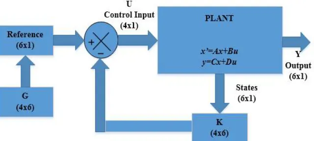
We are now able to design linear controller of the quadrotor system using matrices A, B and C we have found. Any controller design procedure is based on information how inputs and outputs of the plant are connected. Figure 1 illustrates block scheme of the closed loop system with state feedback.

Fig. 1. Block scheme of the state feedback

III.QUADCOPTER STABILIZATION VIA POLE PLACEMENT

From Fig.1 the control input, u, consists of 4 angular velocities, [ ], of rotors and it is formed by the sum of reference input multiplied by the gain matrix G and internal states multiplied by the feedback matrix K. Feedback gain matrix K

would be defined after pole placement procedure of the characteristic equation of the system. The procedure of pole placement set such that the rise time, overshoot and settling time are set in the same manner as in [9-16]. For the system the state feedback control references are pitch, roll angles equal to zero. Using state feedback law the relationship between plant input, u, and reference, ref, is written as (7).

= ∙ − (7)

The system on the figure demonstrates quadcopter structure with input = [ ] and reference = [ ] . To get full correspondence of feedback and reference input there must be some relation, G, that is expressed as follows.

=− ( − ) (8)

̇= ( − ) +

= (9)

So, linear model of the quadrotor system has 12 states, then we expect to find 12 poles of the system. In our test we did not consider positions, so we need to find 6 poles only. Also it is necessary to discretize the model as if it was a real model based on digital microcontroller system. Using corresponding MATLAB functions equations (7), (8), (9) are converted into discrete time form of (10).

= exp( [ ])

= c2d(K)

= ( − )

[ + 1] = ( − ) [ ] + [ ]

[ ] = [ ] (10)

where Pdis poles on Z plan, Ad, Bd, Cd, Kd, Gd are discrete time matrices and x[n], y[n], u[n]are values of the states, outputs and control inputs at n-thtime step correspondingly.

Pole placement method is a method, where for the designed controller should be changed poles of characteristic equation of the mathematical model so that the system desired characteristics such as a settling time, an overshoot and steady state error must be met. Thus, pole placement procedure has three steps. First step is obtaining the denominator from transfer function of the mathematical model of the system to get characteristic equation of the poles. Next is calculation of desired poles basing on requirements of the system. Last step is calculation of feedback coefficients that change poles of the mathematical model to desired ones.

The main problem of state feedback control is the choice of closed loop pole locations. For multiple input systems it is not easy to relate elements of the control matrix K to the positions of the closed loop poles. As such, there is no unique solution K for a set of poles, and choosing the optimum K-values is not trivial. It is known that poles of the system must be chosen in the left half of s plane to insure stability. The procedure of pole placement set such that the rise time, overshoot and settling time are set in the same manner as in [11] using well known formulas (11) under the given conditions.

= ( ⁄ )

( ( ⁄ ))

≈ (11)

IV.SIMULATION AND EXPERIMENTAL RESULTS

We can choose any of many variants of the arrangement of poles using the criterion of dominant poles. From this it follows that positions of the poles can be chosen arbitrarily, but sufficiently small, so that the elements of the matrix K

are reasonable in values. Choosing the values for the poles, it should be borne in mind that the values of the poles can not be too close to each other, otherwise we can face numerical problems when trying to solve this problem. But the real parts of the poles can not be too far from zero, otherwise it would make the controller too complicated in terms of the necessary control inputs.

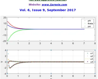
A.Simulation

Fig. 2.Roll (phi), pitch (theta), yaw (psi) angles in the upper graph. Lifting force (u1, u2, u3, u4)

B. Experiments

Our mission is to use state feedback control by pole placement method and make the quadcopter to hover in mid-air. Table 1 below shows constants and values of technical parameters of the quadrotor used for our simulation and experiments and in Fig.3 shown quadcopter designed in our laboratory.

Table I.Quadcopter constants and values

Formula Units Values

g=9.81 [m/s^2 ] gravity constant

m=0.09 [kg] mass of motor

M=0.8-(4m) [kg] mass of body

l=0.22 [m] length of arm

a=0.02 [m] body, inside radius

b=0.22 [m] body, outside radius

Ix=1/2 M(a^2+b_2 )+2l^2 m [kg m^2] inertia in x axes

Iy=1/2 M(a^2+b_2 )+2l^2 m [kg m^2] inertia in y axes Iz=1/2 M(a^2+b_2 )+4l^2 m [kg m^2] inertia in z axes

F=Kt ω^2 [N] force produced by propeller

Ct=0.1154 thrust coefficient

q=1.225 [kg/m^3 ] air density coefficient Dp=0.256 [m] diameter of propeller

Kt=Ct (ρD^4)/(4π^2 ) [kg m^2 〖rad〗^2 ] Force coefficient

M=Km ω^2 [Nm] moment produced by propeller

Cp=0.0743 drag coefficient

Km=Ct (ρD^5)/(8π^2 ) [kg m 〖rad〗^2 ] moment coefficient

Fig. 3. The experimental environment of the quadrotor system

The controller needs feedback information such as positions, orientations and the appropriate parameters (e.g. linear angular velocity) that are measured by sensors. We use MPU-6050 chip that contains MEMS accelerometers and a MEMS gyros. To estimate angles the accelerometer is adjusted to ±2g and to estimate angular velocities the gyroscope is adjusted to ±1000 deg/sec. To determine the response time of BLDC (Fig. 4), we conducted multiple experiments on applied voltage versus speed ratio and lifting force. The experiment is done using propeller 10x4.5 and A2212/13T-KV1000 BLDC and ESC with 30A.

Fig. 4.Lifting force vs duty cycle of PWM relation

Below in Figure 5 shown only few graphical results of many experiments of angular values for roll, pitch, and yawread from the MEMS sensors during the hovering mode.

At arbitrary placement of the six poles p= [-6 -5 -4 -3 -2 -1] we got feedback coefficients as shown below. y = -2.021x2_{+ 22.17x + 38.08}

R² = 0.998

0 10 20 30 40 50 60 70 80 90 100

0 0.5 1 1.5 2 2.5 3 3.5 4

F(N)

=

−0.1157 −0.1023 −0.0458 −0.0181 1.4578 0.5497

−0.0500 −0.0203 −0.1007 −0.0973 −1.4579 −0.5497 0.1160 0.1024 0.0456 0.0180 1.4579 0.5497 0.0497 0.0202 0.1009 0.0974 −1.4579 −0.5497

-15.00 -10.00 -5.00 0.00 5.00 10.00 15.00

0 200 400 600 800 1000 1200 1400 1600 1800 2000

Roll(θ) Pitch(φ) Yaw(ψ)

Time (ms) Angle (deg)

Fig. 5a. Experimental results with p= [-6 -5 -4 -3 -2 -1]

Placing poles at locations p= [-60 -5 -4 -3 -2 -1] we got the feedback coefficients. The first pole is very fast in comparison with the others and it has influence in yaw angle (Fig.5b).

=

−0.1159 −0.1024 −0.0457 −0.0180 . . −0.0498 −0.0202 −0.1008 −0.0973 − . − .

0.1159 0.1024 0.0457 0.0180 . .

0.0498 0.0202 0.1008 0.0973 − . − .

-15.00 -10.00 -5.00 0.00 5.00 10.00 15.00

0 200 400 600 800 1000 1200 1400 1600 1800 2000

Roll(θ) Pitch(φ) Yaw(ψ) Angle (deg)

Time (ms)

Fig. 5b. Experimental results with p= [-60 -5 -4 -3 -2 -1]

At mutually unequal poles, p = [-60 -50 -4 -3 -2 -1], we obtained the following feedback coefficients. More negative poles make the dynamics of regulation faster (Fig. 5c).

=

−0.4509 −0.3050 −0.6411 −0.3177 . . −0.9355 −0.4347 −0.7781 −0.4261 − . − .

0.9448 0.4896 0.6646 0.3191 . .

-20.00 -15.00 -10.00 -5.00 0.00 5.00 10.00 15.00 20.00

0 200 400 600 800 1000 1200 1400 1600 1800 2000

Roll(θ) Pitch(φ) Yaw(ψ)

Time (ms) Angle (deg)

Fig. 5c. Experimental results with p= [-60 -50 -4 -3 -2 -1]

With couples of poles at p= [-40 -40 -3 -3 -2 -2] we got the feedback coefficients shown below and corresponding time diagram is shown in Fig.5d.

=

− . −0.1002 . . 4.3446 1.6064

. . −1.1228 −0.6022 −4.3446 −1.6064

. 0.1002 − . − . 4.3446 1.6064

− . − . 1.1228 0.6022 −4.3446 −1.6064

-15.00 -10.00 -5.00 0.00 5.00 10.00 15.00

0 200 400 600 800 1000 1200 1400 1600 1800 2000

Roll(θ) Pitch(φ) Yaw(ψ)

Angle (deg)

Time (ms)

Fig. 5d.Experimental results with p= [-40 -40 -3 -3 -2 -2]

At the triple poles p= [-40 -40 -40 -3 -3 -3] we got the feedback coefficients. As seen, the coefficients become symmetric (Fig.5e).

=

− . −0.6166 . . 4.3446 1.6064

. . − . −0.6166 −4.3446 −1.6064

. 0.6166 . . 4.3446 1.6064

-15.00 -10.00 -5.00 0.00 5.00 10.00 15.00

0 200 400 600 800 1000 1200 1400 1600 1800 2000

Roll(θ) Pitch(φ) Yaw(ψ)

Angle (deg)

Time (ms)

Fig. 5e. Experimental results with p= [-40 -40 -40 -3 -3 -3]

At poles p= [-30 -30 -30 -3 -3 -3] we got the feedback coefficients which are symmetricand the variances of the parameters become smaller (Fig.5f).

=

−1.3663 −0.5161 . . 3.5597 1.3447

. . −1.3663 −0.5161 −3.5597 −1.3447

1.3663 0.5161 . . 3.5597 1.3447

− . − . 1.3663 0.5161 −3.5597 −1.3447

-15.00 -10.00 -5.00 0.00 5.00 10.00 15.00

0 200 400 600 800 1000 1200 1400 1600 1800 2000

Roll(θ) Pitch(φ) Yaw(ψ)

Angle (deg)

Time (ms)

Fig. 5f. Experimental results with p= [-30 -30 -30 -3 -3 -3]

Using poles p= [-30 -30 -30 -1 -1 -1] we got the feedback coefficient which are symmetric and the parameter variances are stabilized more (Fig. 5g).

=

−0.4646 −0.4852 . . 1.2104 1.2641

. . −0.4646 −0.4852 −1.2104 −1.2641

0.4646 0.4852 . . 1.2104 1.2641

-15.00 -10.00 -5.00 0.00 5.00 10.00 15.00

0 200 400 600 800 1000 1200 1400 1600 1800 2000

Roll(θ) Pitch(φ) Yaw(ψ)

Time (ms) Angle (deg)

Fig. 5g. Experimental results with p= [-30 -30 -30 -1 -1 -1]

It was seen that with three slow and three fast poles located relatively far each other the angles are stabilized more and more. All the poles are now located on the left half of the complex plane, they all have a negative real part.

VI.CONCLUSION

Advantage of pole placement method is that the controller designed by this method can be easily expanded to an optimal or adaptive controller. In this work were developed all stages of the control system starting from the analysis of the quadcopter as a flying object and the mathematical model was created and modified for using in design purposes. After choosing appropriate poles, the control system for the quadcopter was implemented in the real quadcopter. Experiments for estimation theoretical results were fulfilled.

We can select the desired poles of the system around the dominant poles. The slowest poles are the dominant poles and they have influence on angular values. As seen from the experimental results number of dominant poles (in our case 3 poles) must be equal to number of main parameters such as yaw, pitch and roll angles. Coefficients of feedback gain matrix K for the system are calculated during the simulation in MATLAB. It was seen that appropriate choice of the poles leads to generate coefficients of the matrix so that each column of the matrix includes pair of coefficients with opposite sign and pair of zeros except last two columns which correspond to yaw angle.However, in practical application placing them too far to the left the result have greater error, which can be unsafe in physical implementation of the controller and lead to instability. Further, too high gain, K, will amplify any unwanted noise that the system experiences which can also lead to instability.

We could, in principle, arbitrarily place the poles of the closed-loop system to achieve the desired system response. Unfortunately, what we can accomplish in simulation may not coincide with what we can accomplish in practice.The real control system of hovering quadcopter obtained from simulation and experiments shows adequate results.

REFERENCES

[1] Teppo Luukkonen. Modelling and control of quadcopter.School of Science. Independent research project in applied mathematics Espoo, August 22, 2011. Aalto University

[2] T. Bresciani, "Modelling, identification and control of a quadrotor helicopter, " Ph.D. dissertation, Lund University, 2008

[3] Andrew Gibiansky.Quadcopter Dynamics and Simulation, Sep 2015, [online] Available:

http://andrew.gibiansky.com/blog/physics/quadcopter-dynamics

[4] L.M. Argentim, W.C. Rezende, P.E. Santos and R.A. Aguiar. PID, LQR and LQR-PID on a quadcopter platform In Proc. of the International Conference on Informatics, Electronics and Vision (ICIEV), pages 1- 6, 2013

[5] Katherine Karwoski. Quadrocopter Control Design and Flight Operation. NASA USRP – Internship Final Report. Marshall Space Flight Center. May 2011

[7] Heba talla Mohamed Nabil ElKholy, “Dynamic Modeling and Control of a Quadrotor Using Linear and Nonlinear Approaches” American University in Cairo, 2014

[8] Beard, Randal, "Quadrotor Dynamics and Control Rev 0.1" (2008). All Faculty Publications. Paper 1325.

http://scholarsarchive.byu.edu/facpub/1325

[9] D. Zhang, H. Qi, X. Wu, Y. Xie, J. Xu, "The Quadrotor Dynamic Modeling and Indoor Target Tracking Control Method", Mathematical Problems in Engineering, vol. 2014, no. 9, 2014

[10] Xiaodong Zhang,1 Xiaoli Li,2 Kang Wang,2 and Yanjun Lu, “A Survey of Modelling and Identification of Quadrotor Robot”, Abstract and Applied Analysis, Volume 2014, Article ID 320526, 16 pages

[11] http://ocw.mit.edu/terms. MIT OpenCourseWare. 2.004 Dynamics and Control II. Spring 2008. [12] K. Ogata, Modern Control Engineering, Prentice Hall, New York, NY, USA, 2002.

[13] Alberto Bemporad. Linear State Feedback Control. University of Trento. 2010-2011.

http://cse.lab.imtlucca.it/~bemporad/teaching/ac/pdf/05b-pole-placement.pdf

[14] Tserendondog Tengis, Amar Batmunkh. Quadcopter stabilization using state feedback controller by pole placement method / 01. International Journal of Internet, Broadcasting and Communication_ Vol.9 No.1 (2017)

[15] A. A. Wahab, M. Rosbi and S. S. Syariful, "The Effectiveness of Pole Placement Method in Control System Design for an Autonomous Helicopter Model in Hovering Flight," International Journal of Integrated Engineering, vol. 1, Dec. 2011, pp. 33-46

[16] A. Lebedev, "Design and Implementation of a 6DOF Control System for an Autonomous Quadrocopter”. Master Thesis. Aerospace Information Technology’ Department, University of Würzburg, 07- 09- 2013

[17] Graeme N. Wilson, Alejandro Ramirez-Serrano, and Qiao Sun, “Vehicle Parameter Independent Gain Matrix Selection for a Quadrotor using State-Space Controller Design Methods” 11th International Conference on Informatics in Control, Automation and Robotics Vienna University of Technology September 1-3, 2014, Vienna, Austria

[18] A.A.J.Lefeber. Controlling of a single drone. Hovering the drone during flight modes. TU/E Eindhoven. Department of mechanical engineering. Dynamics and control. Aug 2015.

[19] Tom´aˇs Krajn´ık, Vojtˇech Von´asek, Daniel Fiˇser, and Jan Faigl. AR-Drone as a Platform for Robotic Research and Education The Gerstner Laboratory for Intelligent Decision Making and Control Department of Cybernetics, Faculty of Electrical Engineering. Czech Technical University in Prague. 2011.

[20] Dirman Hanafi, Mongkhun Qetkeaw, Rozaimi Ghazali, Mohd Nor Mohd Than, Wahyu Mulyo Utomo, Rosli Omar. Simple GUI Wireless Controller of Quadcopter. Department of Mechatronic and Robotic Engineering, Department of Power Engineering, Faculty of Electrical and Electronic Engineering. University Tun Hussein Onn Malaysia.

[21] M. Eswaran, P, M Guda, M Priya et al., "Stabilization of UAV Quadcopter", Proceedings of the International Conference on Soft Computing Systems, 2016

[22] A. Tayebi, S. McGilvray, "Attitude stabilization of a four-rotor aerial robot: Theory and experiments", IEEE Trans. Control Syst. Technol., vol. 14, no. 3, pp. 562-571, May 2006.

[23] Stephen Armah, 1 Sun Yi, 2Wonchang Choi and 2Dongchul Shin, “Feedback Control of Quad-Rotors with a Matlab-Based Simulator” American Journal of Applied Sciences 2016

[24] Tengis Tserendondog, Byambajav Ragchaa, Luubaatar Badarch, Batmunkh Amar “State Feedback Control of Unbalanced Seesaw” The 11th International Forum on Strategic Technology 2016

[25] S. Bouabdallah et al., "Design and control of an indoor micro quadrotor", Proc. (IEEE) International Conference on Robotics and Automation (ICRA'04), 2004

[26] Tahir Z, Jamil M, Liaqat SA, Mubarak L, Tahir W, Gilani SO. State space system modeling of a quad copter UAV. Indian Journal of Science and Technology. 2016 Jul; 9(27):1–5